From Pixels to Sentiment: Fine-tuning CNNs for Visual Sentiment ...

arXiv:1604.03489v1 [cs.CV] 12 Apr 2016

From Pixels to Sentiment: Fine-tuning CNNs for Visual Sentiment Prediction

Victor Campos Universitat Politecnica de Catalunya (UPC) Barcelona, Catalonia/Spain [email protected] Brendan Jou Columbia University New York, NY USA [email protected]

Xavier Giro-i-Nieto Universitat Politecnica de Catalunya (UPC) Barcelona, Catalonia/Spain [email protected]

Abstract Visual media have become a crucial part of our social lives. The throughput of generated multimedia content, together with its richness for conveying sentiments and feelings, highlights the need of automated visual sentiment analysis tools. We explore how Convolutional Neural Networks (CNNs), a computational learning paradigm that has shown outstanding performance in several vision tasks, can be applied to the task of visual sentiment prediction by fine-tuning a state-of-the-art CNN. We analyze its architecture, studying several performance boosting techniques, which led to a network tuned to achieve a 6.1% absolute accuracy improvement over the previous state-of-the-art on a dataset of images from a popular social media platform. Finally, we present visualizations of local patterns that the network associates to each image’s sentiment.

1

Introduction

The amount of user-generated multimedia content that is uploaded to social networks every day has experienced an impressive growth in the last few years. They are the means by which most of their users express their feelings and opinions about nearly every event in their lives. Moreover, visual contents have become a very natural and rich media to share emotions and sentiments. Affective Computing [18] is lately drawing the attention of researchers from different fields, including robotics, entertainment and medicine. This increasing interest can be attributed to the numerous successful applications, such as emotional understanding of viewer responses to advertisements using facial expressions [15] and monitoring of emotional patterns to help patients suffering from mental health disorder [8]. However, due to the complexity of the task, the understanding of image and video processing techniques for automatic sentiment and emotion detection in multimedia is still far from other computer vision tasks where machines are approaching or have exceeded human performance. The state-of-the-art in fundamental vision tasks has recently undergone a great performance improvement thanks to Convolutional Neural Networks (CNNs) [12], fact that led us to explore the potential of transferring these techniques to a more abstract task such as visual sentiment prediction, i.e. automatically determining the sentiment (either positive or negative) that an image would provoke to a human viewer. Given the difficulty of collecting large-scale datasets with reliable sentiment annotations, our efforts focus on understanding domain-transferred CNNs for visual sentiment prediction by analyzing the performance of a state-of-the-art architecture fine-tuned for this task. 1

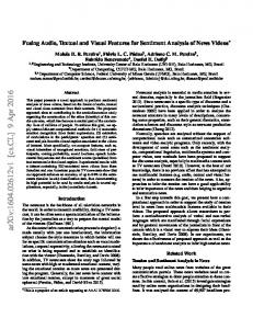
Figure 1: Overview of the proposed visual sentiment prediction framework. In this paper, we extend our previous work in [3]. Our contributions include: (1) a visual sentiment prediction framework that outperforms the state-of-the-art approach on an image dataset collected from Twitter, (2) a rigorous analysis of the CNN architecture by studying the performance evolution along its layers and performing network architecture surgery, (3) a study of the weights initialization’s impact by changing the original domain from which the learning is transferred from, and (4) a visualization of the local image regions that contribute to the overall sentiment prediction. The trained models and necessary tools to replicate our experiments are publicly available at https://github.com/imatge-upc/sentiment-2016.

2

Related Work

Computational affective understanding for visual multimedia has been an area of research interest in several in the past few years and resulted in the development of a number of handcrafted feature representations. Color Histograms and SIFT-based Bag-of-Words, common low-level image descriptors used in vision recognition tasks, were evaluated in [21] for the task of visual sentiment prediction. Given the close relationship between Art and Psychology, some other research has also employed visual descriptors inspired by artistic disciplines to visual emotion classification [14] and automatic image adjustment of emotional reactions [17]. In [2] and [10], a Visual Sentiment Ontology consisting of adjective-noun pairs (ANPs) was proposed as a mid-level representation to bridging the affective gap between low-level visual features and high-level affective semantics. A bank of detectors was also proposed in [2] and [10], called SentiBank and MVSO, respectively, that can automatically extract these mid-level representations. The suitability of Convolutional Neural Networks (CNNs) for some computer vision tasks was studied in the past [12]. Nevertheless, it has been the creation of large-scale datasets such as [6] and the rise of graphical processing units (GPUs) that has led them to show outstanding performance in several vision tasks [7, 11, 22]. They have been proven very effective in transfer learning experiments [16] when the lack of data prevents training them from scratch. This important attribute of CNNs was explored for the task of visual sentiment prediction in [25], where it was shown that off-the-shelf visual descriptors could outperform hand-crafted low-level features and SentiBank [2]. The performance of CNNs for visual sentiment prediction was further explored in [26], where a custom CNN was designed for visual sentiment prediction, but very little intuition for why their network would improve on the state-of-the-art architectures was given. In this work, we pre-train with a classical, but proven CNN and develop a thorough analysis of the network in order to gain insight in the design and training of CNNs for the task of visual sentiment prediction.

3

Methodology

The CNN architecture employed in our experiments is CaffeNet, an AlexNet-styled network that differs from the ILSVRC2012 winning architecture [11] in the order of the pooling and normalization layers. As depicted in Figure 2, this CNN is composed by five convolutional layers and three fully connected layers. The rectified linear unit (ReLU) non-linearity, f (x) = max(0, x), is used 2

Figure 2: The template Convolutional Neural Network architecture employed in our experiments. It is an AlexNet-styled architecture adapted for visual sentiment prediction.

as the activation function. The first two convolutional layers are followed by max-pooling and local response normalization layers, while conv5 is followed by a max-pooling layer. Finally, the output of the last fully connected layer, fc8, is fed to a softmax function that computes the probability distribution over the different classes. The experiments were performed using Caffe [9], a publicly available deep learning framework. The Twitter dataset that was collected and released by the authors in [26] is used in order to train and evaluate the performance of our fine-tuned CaffeNet in the task of visual sentiment prediction. In contrast with other annotation methods which rely on image metadata, each one of the 1,269 images in the dataset were labeled into positive or negative sentiment by five human annotators. This results in a more accurate ground truth, which allows the network to learn better and stronger sentimentrelated concepts. We use only the subset of images that built consensus among the five annotators, namely five-agree subset. The 880 images in the five-agree subset were divided into five different folds in order obtain more statistically meaningful results by applying cross-validation.

3.1

Fine-tuning CaffeNet for Visual Sentiment

Convolutional Neural Networks (CNNs) contain an enormous number of parameters that need to be tuned, so they often require large datasets to be trained from scratch. This requirement becomes critical in tasks such as visual sentiment prediction, where there is a wide variability in visual content composing a positive or negative class. In addition, for visual sentiment prediction tasks, the size of the datasets is usually constrained because of the difficulty and expense of acquire high-quality labels that depend so much on subjective reasoning. Previous works [16, 20, 1] have successfully dealt with this latter problem by fine-tuning instead of training the network from scratch. The finetuning strategy consists in initializing all the weights in the network, except the ones in the last layer, using a pre-trained model instead of using a random initialization. The last fully connected layer is then discarded and replaced by a new one, usually containing the same amount of neurons as classes in the dataset, with a random initialization of their weights. Finally, the training process is started using the data from the target dataset. The main advantages of this procedure compared to a random initialization of all the weights are (1) a faster convergence, since the gradient descent algorithm starts from a point which is much closer to a local minimum, and (2) a reduction in the overfitting likelihood when the training dataset is small. Besides, in a transfer learning setting where the original and target domains are similar, pre-training can be seen as additional training data from which the network may benefit to achieve a better performance. As shown in Figure 2, the original fc8 in CaffeNet is replaced by a two-neuron layer, fc8 twitter, since the addressed task distinguishes between two classes: positive and negative sentiment. The weights in this new layer are initialized from a zero-mean Gaussian distribution with standard deviation 0.01, while the biases are initially set to zero. The rest of layers are initialized using a model pre-trained on the ILSVRC2012. The network is trained using stochastic gradient descent, momentum of 0.9 and an initial base learning rate of 0.001 that is divided by 10 every 6 epochs. In order to compensate the fact that the weights in the last layer are not initialized using a pre-trained model, their individual learning rate is set 10 times higher than the base one. Each model is trained during 65 epochs, i.e. the CNN sees each training image 65 times, using mini-batches of 256 randomly sampled images each. 3

A technique that has proven useful in tasks such as object recognition by previous works [4] is oversampling, which consists in feeding slightly modified versions of the image (e.g. by applying flips and crops) to the network, as it helps to deal with the dataset bias [24]. We explore the effectiveness of this strategy for the task of visual sentiment prediction by feeding 10 different combinations of flips and crops of the original image to the CNN in the test stage. The classification scores for each combination are fused using an average operation in order to determine the final decision. 3.2

Layer by layer analysis

Convolutional Neural Networks are complex learning systems. The optimization problem of designing high performing architectures using as few resources as possible is an ongoing area of research. In this section, we present a series of experiments to analyze the contribution of the individual layers of the fine-tuned CaffeNet for the task of visual sentiment prediction. Despite the output of the studied CNN is the probability of the image belonging to one of the two classes, i.e. positive or negative sentiment, it is possible to extract the individual activations at each layer of the architecture and use them as visual descriptors. Previous works have used the activations from individual layers as visual descriptors to solve different vision tasks [20, 19], although only fully connected layers are usually used for this purpose. We further extend this idea and train classifiers using activations from all the layers in the architecture, as depicted in Figure 3, so it is possible to compare the effectiveness of the different representations that are learned along the network. Feature maps from convolutional, pooling and normalization layers were flattened into d-dimensional vectors before being used to train the classifiers. Two different classifiers were considered: Support Vector Machine (SVM) with linear kernel and Softmax. The regularization parameter of each classifier was optimized by cross-validation.

Figure 3: Experimental setup for the layer analysis using linear classifiers. Activations in each layer are used as visual descriptors in order to train a classifier.

3.3

Layer ablation

While convolutional layers share weights in order to reduce the amount of hyperparameters in the model, fully connected layers are densely connected, so they contain most of the weights in the architecture. Therefore, the excess of units of this type may lead the model to poorer generalization capabilities [4, 27]. In our experiments, we explore how the ablation of fully connected layers and, consequently, a large percentage of the architecture’s parameters, affects the performance of fine-tuned CNNs for the task of visual sentiment prediction. Four different architectures are studied, as depicted in Figure 4, where the last or the two last fully connected layers are removed. Two different strategies, which are described in the following subsections, were followed when removing layers from the original architecture. 4

Figure 4: Layer ablation architectures. Networks fc7-4096 and fc6-4096 keep the original configuration after ablating the layers in the top of the architecture (Section 3.3.1), while in fc7-2 and fc6-2 the last remaining layer is replaced by a two-neuron layer (as described in Section 3.3.2). The dimension of each layer’s output is indicated between brackets. 3.3.1

Raw ablation

In this first layer ablation strategy, the architecture that remains after removing the top layers is kept unmodified. Two different architectures are studied, fc7-4096 and fc6-4096 in Figure 4, where the last and the two last layers have been removed, respectively. In this set of experiments some of the weights that connect the two last layers are not used, but this approach allows to study whether the network is capable of adapting to the new task without needing to randomly initialize some of its parameters. All the weights are loaded from the pre-trained model and, since none of them are randomly initialized, there is no layer that needs a larger learning rate. The rest of training conditions are the same as in Section 3.1. 3.3.2

2-neuron on top

Inspired by the fine-tuning methodology explained in Section 3.1, where the last layer always contains as many units as classes in the dataset, we replaced the last remaining layer by one with 2 neurons, one for positive and another for negative sentiment, obtaining architectures fc7-2 and fc6-2 in Figure 4. The weights in the last layer are initialized from a zero-mean Gaussian distribution with standard deviation 0.01, while the biases are set to zero. The rest of parameters are loaded from the pre-trained model. The learning rate of the last layer is set to be 10 times higher than the base learning rate to compensate the fact that their weights are randomly initialized. The rest of training conditions are the same as in Section 3.1 except for the learning rate of architecture fc6 2, which was set to 0.0001 in order to avoid divergence. 3.4

Initialization analysis

Given its success in ILSVRC2012, AlexNet-styled CNNs have been used for several vision tasks other than object recognition, such as scene recognition [28] or adjective-noun pair detection [5, 10]. Since fine-tuning a CNN can be seen as a transfer learning strategy, we explored how changing the original domain affects the performance by using different pre-trained models as initialization for the fine-tuning process, while keeping the architecture fixed. In addition to the model trained on ILSVRC 2012 [11] (i.e. CaffeNet), we evaluate models trained on Places dataset [28] (i.e. PlacesCNN), which contains images annotated for scene recognition, and two sentimentrelated datasets: Visual Sentiment Ontology (VSO) [2] and Multilingual Visual Sentiment Ontology (MVSO) [10], which are used to train adjective-noun pair (ANP) detectors that are later used as a mid-level representation to predict the sentiment in an image. The model trained on VSO, DeepSentiBank [5], is a fine-tuning of CaffeNet on VSO. Given the multicultural nature of MVSO, there is one model for each language (i.e. English, Spanish, French, Italian, German and Chinese) and each one of them is obtained by fine-tuning DeepSentiBank on a specific language subset of MVSO. All models are fine-tuned for 65 epochs, following the same procedure as in Section 3.1. 3.5

Going deeper: layer addition

The activations in a pre-trained CNN’s last fully connected layer contain the likelihood for the input image belonging to each class in the original training dataset, but the regular fine-tuning strategy completely discards this information. Besides, since fully connected layers contain most of the weights in the architecture, a large amount of parameters that may contain useful information for the target task are being lost. 5

In this set of experiments we explore how adding high-level information by reusing the last layer of pre-trained CNNs affects their performance when fine-tuning for visual sentiment prediction. In particular, the networks pre-trained on ILSVRC2012 (i.e. CaffeNet) and MVSO-EN are studied. The former was originally trained to recognize 1,000 object classes, whereas the latter was used to detect 4,342 different Adjective Noun Pairs that were designed as a mid-level representation for visual sentiment prediction. A 2-neuron layer, namely fc9 twitter, is added on top of both architectures (Figure 5). The weights in this new layer are initialized from a zero-mean Gaussian distribution with standard deviation 0.01, while the biases are set to zero. The parameters in the rest of layers are loaded from the pre-trained models. The individual learning rate of fc9 twitter is set to be 10 times higher than the base learning rate to compensate for the random initialization of its parameters. The rest of training conditions are the same as described in Section 3.1.

Figure 5: Layer addition architectures. The dimension of each layer’s output is indicated between brackets.

3.6

Visualization: fully convolutional network

A very natural way to gain insight about the concepts learned by the network consists in observing which parts of an image lead the CNN to classify it either as positive or negative. We convert the fine-tuned CaffeNet into a fully convolutional network by replacing its fully connected layers by convolutional layers (see Table 1 for details), following the method described in [13] and reusing the weights from the original fully connected layers for the fully convolutional architecture, so no further training is needed. Since the original architecture contains fully connected layers that implement a dot product operation, it requires the input to have a fixed size. In contrast, the fully convolutional network can handle inputs of any size: by increasing the input size, the dimensions of the output will increase as well and it will become a prediction map on overlapping patches from the input image. We generate 8×8 prediction maps for the images of the Twitter five-agree dataset by using inputs of size 451×451 instead of 227×227, which were the required input dimensions of the original architecture.

4

Experimental results

This section contains the results for the experiments described in Section 3, as well as intuition and conclusions for such results.

Table 1: Details of new convolutional layers resulting from converting our modified CaffeNet to a fully convolutional network (stride=1). Layer fc6-conv fc7-conv fc8 twitter-conv

Number of kernels 4096 4096 2

6

Kernel size (h × w × d) 6 × 6 × 256 1 × 1 × 4096 1 × 1 × 4096

Table 2: Five-fold cross-validation results on Twitter dataset. Model Baseline PCNN from [26] Fine-tuned CaffeNet Fine-tuned CaffeNet with oversampling

4.1

Five-agree 0.783 0.817 ± 0.038 0.830 ± 0.034

Four-agree 0.714 0.782 ± 0.033 0.787 ± 0.039

Three-agree 0.687 0.739 ± 0.033 0.749 ± 0.037

Fine-tuning CaffeNet for Visual Sentiment

The five-fold cross-validation results for the fine-tuning experiment on Twitter dataset are detailed in Table 2, together with the best five-fold cross-validation result in this dataset from [26]. The latter was achieved using a custom architecture, composed by two convolutional layers and four fully connected layers, that was trained using the Flickr dataset (VSO) [2] and later fine-tuned on Twitter dataset. In order to evaluate the performance of our approach when using images with more ambiguous annotations, CaffeNet was also fine-tuned on four-agree and three-agree subsets, i.e. those containing images that built consensus among at least four and three annotators, respectively. These results show that, despite being pre-trained for a completely different task, the AlexNetstyled architecture clearly outperforms the custom architecture from [26]. This difference suggests that visual sentiment prediction architectures may benefit from an increased depth that comes from adding a larger amount of convolutional layers instead of fully connected ones, as suggested by [27] for the task of object recognition. Secondly, this results highlight the importance of high-level representations for the addressed task, as transferring learning from object recognition to sentiment prediction results in high accuracy rates. Averaging over the predictions of modified versions of the image results in an additional performance boost, as found out by the authors in [4] for the task of object recognition. This fact suggests that oversampling helps to compensate the dataset bias and increases the generalization capability of the system without a penalization on the prediction speed thanks to the batch computation capabilities of GPUs. 4.2

Layer by layer analysis

The results for the layer-wise analysis using linear classifiers are compared in Table 3. The evolution of the accuracy rates at each layer, for both SVM and Softmax classifiers, show how the learned representation becomes more effective along the network. While every single layer does not introduce a performance boost with respect to the previous ones, it does not necessarily mean that the architecture needs to be modified: since the training of the network is performed in an end-to-end manner, some of the layers may apply a transformation to their inputs from which later layers may benefit, e.g. conv5 and pool5 report lower accuracy than the previous conv4 when used directly for classification, but the fully connected layers on top of the architecture may be benefiting from their effect since they produce higher accuracy rates than conv4. Previous works have studied the suitability of Support Vector Machines to classify off-the-shelf visual descriptors extracted from pre-trained CNNs [19], while some others have even trained these networks using the L2-SVM’s squared hinge loss on top of the architecture [23]. From our layer by layer analysis, it is not possible to claim that one of the classifiers consistently outperforms the other for the task of visual sentiment prediction, at least using the proposed CNN in the Twitter five-agree dataset. 4.3

Layer ablation

The five-fold cross-validation for the fine-tuning of the ablated architectures are shown in Table 4. Following the behavior observed in the layer-wise analysis with linear classifiers in Section 4.2, removing layers from the top of the architecture results in a deterioration of the classification accuracy. These results suggest that placing a two-neuron layer on top of the architecture is a better solution than the strategy of keeping the original architecture unmodified after ablating the top layers. It is important to notice that during training, raw ablation architectures have a larger amount of param7

Table 3: Layer analysis with linear classifiers: Five-fold cross-validation results on five-agree Twitter dataset. Layer SVM Softmax fc8 0.82 ± 0.055 0.821 ± 0.046 fc7 0.814 ± 0.040 0.814 ± 0.044 fc6 0.804 ± 0.031 0.81 ± 0.038 pool5 0.784 ± 0.020 0.786 ± 0.022 conv5 0.776 ± 0.025 0.779 ± 0.034 conv4 0.794 ± 0.026 0.781 ± 0.020 conv3 0.752 ± 0.033 0.748 ± 0.029 norm2 0.735 ± 0.025 0.737 ± 0.021 pool2 0.732 ± 0.019 0.729 ± 0.022 conv2 0.735 ± 0.019 0.738 ± 0.030 norm1 0.706 ± 0.032 0.712 ± 0.031 pool1 0.674 ± 0.045 0.68 ± 0.035 conv1 0.667 ± 0.049 0.67 ± 0.032 Table 4: Layer ablation: Five-fold cross-validation results on five-agree Twitter dataset. Architecture Without oversampling With oversampling Parameter reduction fc7-4096 0.759 ± 0.023 0.786 ± 0.019 8194 fc6-4096 0.657 ± 0.040 0.657 ± 0.040 >16M fc7-2 0.784 ± 0.024 0.797 ± 0.021 >16M fc6-2 0.651 ± 0.044 0.676 ± 0.029 >54M eters to tune compared to their counterparts with two-neuron layers on top, whereas they both use the same amount of weights during inference, i.e. most of the neurons in the last layer of raw ablation architectures are being ignored during the test stage. The superiority of the latter method was confirmed by further research, which showed that architecture fc6-4096 always predicts towards the majority class, i.e. positive sentiment. If we compare the architectures with a two-neuron layer on top, we observe that the reduction in accuracy is larger in architecture fc6-2, where the convergence from 9,216 neurons in pool5 to a two-layer neuron might be too sudden. This is not the case of architecture fc7-2, where the removal of more than 16M parameters produces only a slight deterioration in performance. These observations suggest that an intermediate fully connected layer that provides a softer dimensionality reduction is beneficial for the architecture, but the addition of a second fully connected layer between pool5 and the final two-neuron layer produces a small gain compared to the extra 16M parameters that are being added. This trade-off is especially important for tasks such as visual sentiment prediction, where collecting large datasets with reliable annotations is difficult, and removing one of the fully connected layers in the architecture might allow training it from scratch using smaller datasets without overfitting the model. 4.4

Initialization analysis

Convolutional Neural Networks that are trained from scratch using large-scale datasets usually achieve very similar results regardless of their initialization, but the fact of fine-tuning on a reduced dataset with low learning rates seems to increase the influence of the original model on the final performance, as seen in the results for the different initializations presented in Table 5. These numerical results show how most of the models that were already trained for a sentimentrelated task outperform the ones pre-trained on ILSVRC 2012 and Places, whose images are mostly neutral in terms of sentiment. The MVSO-ZH model leads to the worst performance among all the tested initializations. The authors in [26] observed that using a Chinese-specific model to predict the sentiment in other languages reported the worst results in all their cross-lingual domain transfer experiments. Given the way in which the Twitter dataset used in our experiments was collected, it is very likely that most of the annotators were not Chinese and it may be the reason why the MVSO-ZH model produces lower accuracy rates than the rest of MVSO models. 8

Table 5: Five-fold cross-validation results for the different initializations on five-agree Twitter dataset. Pre-trained model CaffeNet PlacesCNN DeepSentiBank MVSO [EN] MVSO [ES] MVSO [FR] MVSO [IT] MVSO [DE] MVSO [ZH]

Without oversampling 0.817 ± 0.038 0.823 ± 0.025 0.804 ± 0.019 0.839 ± 0.029 0.833 ± 0.024 0.825 ± 0.019 0.838 ± 0.020 0.837 ± 0.025 0.797 ± 0.024

With oversampling 0.830 ± 0.034 0.823 ± 0.026 0.806 ± 0.019 0.844 ± 0.026 0.844 ± 0.026 0.828 ± 0.012 0.838 ± 0.012 0.837 ± 0.033 0.806 ± 0.020

A comparison of the evolution of the loss function of the different models during training can be seen in Figure 6, where it can be observed that the different pre-trained models need a different amount of iterations until convergence. The DeepSentiBank model seems to adapt worse than other models to the target dataset albeit being pre-trained for sentiment-related task, as can be seen both in its final accuracy and in its noisy and slow evolution during training. On the other hand, the different MVSO models not only provide the top accuracy rates, but converge faster and in a smoother way as well. 4.5

Going deeper: Layer addition

Accuracy results for the layer addition experiments, which are compared in Table 6, show that the accuracy achieved by reusing all the information in the original models is poorer than when performing a regular fine-tuning. One possible reason for the performance deterioration with respect to the regular fine-tuning is the actual information that is being reused by the network. For instance, the CaffeNet model was trained on ILSVRC 2012 for object recognition, e.g. teapot, ping-pong ball or apron, that are mostly neutral in terms of sentiment. This is not the case of MVSO-EN, which was originally used to detect sentiment-related concepts such as nice car or dried grass, but there may be a mismatch between the concepts in the original and target domains that would justify the low accuracy rates. Moreover, the MVSO-EN CNN was originally designed as a mid-level representation, i.e. a concept detector that serves as input to a sentiment classifier. This is not being fulfilled when fine-tuning all the weights in the network, so we speculate that freezing the pre-trained layers and learning only the new weights introduced by fc9 twitter may result in a better use of the concept detector and, thus, a boost in performance.

Figure 6: Comparison of the evolution of the loss function on one of the folds during training. 9

Table 6: Layer addition: 5-fold cross-validation results on 5-agree Twitter dataset. Architecture Without oversampling With oversampling CaffeNet-fc9 0.795 ± 0.023 0.803 ± 0.034 MVSO-EN-fc9 0.702 ± 0.067 0.694 ± 0.060

Figure 7: Some examples of the global and local sentiment predictions of the fine-tuned MVSO-EN CNN. The color of the border indicates the predicted sentiment at global scale, i.e. green for positive and red for negative. The heatmaps in the second row follow the same color code, but they are not binary: a higher intensity means a stronger prediction towards the represented sentiment. 4.6

Visualization

Some examples of the visualization results obtained using the fine-tuned MVSO-EN CNN, which is the top performing model among all that have been presented in this work, are depicted in Figure 7. They were obtained by resizing the 8×8 prediction maps in the output of the fully convolutional network to fit each image’s dimensions. Nearest-neighbor interpolation was used in the resizing process, so that the original prediction block were not blurred. The probability for each sentiment, originally in the range [0,1], was scaled to the range [0, 255] and assigned to one RGB channel, i.e. green for positive and red for negative. It is important to notice that this process is equivalent to feeding 64 overlapped patches of the image to the regular CNN and then composing their outputs to build and 8×8 prediction map, but in a much more efficient manner (while the output dimension is 64 times larger, the inference time grows only by a factor of 3). As a consequence, the global prediction by the regular CNN is not the average of the 64 local predictions in the heatmap, but it is still a very useful method to understand the concepts that the model associates to each sentiment. From the observation of both global and local predictions, we observe two sources of errors that may be addressed in future experiments. Firstly, a lack of granularity in the detection of some high-level semantics is detected, e.g. the network seems unable to tell a campfire from a burning building, and associates them to the same sentiment. On the other hand, the decision seems to be driven mainly by the main object or concept in the image, whereas the context is vital for the addressed task. The former source of confusion may be addressed in future research by using larger datasets, while the latter may be improved by using other types of neural networks or using mid-level representations instead of an end-to-end prediction.

5

Conclusions and future work

We presented an extensive set of experiments comparing several fine-tuned CNNs for the task of visual sentiment prediction. We have shown that deep architectures can learn useful features in recognizing visual sentiment in social images, and in particular, we presented several models that outperform the current state-of-the-art on a dataset of Twitter photos. Some of these models actually performed better even with a smaller number of parameters with respect to the original architecture, highlighting the importance of finding a correct balance in network design when the target task labels can come from a subjective and noisy source. We also showed that the choice of model pre-training initialization can make a difference as well when the target dataset is small. To better 10

understand these models, we presented a sentiment prediction visualization with spatial localization that helped further diagnose erroneous classifications as well as better understand learned network representations. In the future, we plan to study different network architectures for visual sentiment analysis. In addition, we will seek to expand our analysis to larger and weakly supervised settings as well as develop models that can still learn with high fidelity under noisy labels.

Acknowledgments This work has been developed in the framework of the project BigGraph TEC2013-43935-R, funded by the Spanish Ministerio de Econom´ıa y Competitividad and the European Regional Development Fund (ERDF). The Image Processing Group at the UPC is a SGR14 Consolidated Research Group recognized and sponsored by the Catalan Government (Generalitat de Catalunya) through its AGAUR office. We gratefully acknowledge the support of NVIDIA Corporation with the donation of the GeForce GTX Titan Z and X used in this work.

References [1] P. Agrawal, R. Girshick, and J. Malik. Analyzing the performance of multilayer neural networks for object recognition. In European Conference on Computer Vision (ECCV), 2014. [2] D. Borth, R. Ji, T. Chen, T. Breuel, and S.-F. Chang. Large-scale visual sentiment ontology and detectors using adjective noun pairs. In ACM Conference on Multimedia (MM), 2013. [3] V. Campos, A. Salvador, X. Gir´o-i Nieto, and B. Jou. Diving deep into sentiment: Understanding fine-tuned CNNs for visual sentiment prediction. In Proceedings of the 1st International Workshop on Affect & Sentiment in Multimedia (ASM). ACM, 2015. [4] K. Chatfield, K. Simonyan, A. Vedaldi, and A. Zisserman. Return of the devil in the details: Delving deep into convolutional nets. In British Machine Vision Conference (BMVC), 2014. [5] T. Chen, D. Borth, T. Darrell, and S.-F. Chang. DeepSentiBank: Visual sentiment concept classification with deep convolutional neural networks. 2014. [6] J. Deng, W. Dong, R. Socher, L.-J. Li, K. Li, and L. Fei-Fei. ImageNet: A large-scale hierarchical image database. In IEEE Conference on Computer Vision and Pattern Recognition (CVPR), 2009. [7] K. He, X. Zhang, S. Ren, and J. Sun. Delving deep into rectifiers: Surpassing human-level performance on imagenet classification. In IEEE Conference on Computer Vision and Pattern Recognition (CVPR), 2015. [8] S. T.-Y. Huang, A. Sano, and C. M. Y. Kwan. The moment: A mobile tool for people with depression or bipolar disorder. In ACM International Joint Conference on Pervasive and Ubiquitous Computing: Adjunct Publication, 2014. [9] Y. Jia, E. Shelhamer, J. Donahue, S. Karayev, J. Long, R. Girshick, S. Guadarrama, and T. Darrell. Caffe: Convolutional architecture for fast feature embedding. In ACM Conference on Multimedia (MM), 2014. [10] B. Jou*, T. Chen*, N. Pappas*, M. Redi*, M. Topkara*, and S.-F. Chang. Visual affect around the world: A large-scale multilingual visual sentiment ontology. In ACM Conference on Multimedia (MM), 2015. [11] A. Krizhevsky, I. Sutskever, and G. E. Hinton. ImageNet classification with deep convolutional neural networks. In Advances in Neural Information Processing Systems (NIPS), 2012. [12] Y. LeCun, L. Bottou, Y. Bengio, and P. Haffner. Gradient-based learning applied to document recognition. In Proceedings of the IEEE, 1998. [13] J. Long, E. Shelhamer, and T. Darrell. Fully convolutional networks for semantic segmentation. In IEEE Conference on Computer Vision and Pattern Recognition (CVPR), 2015. [14] J. Machajdik and A. Hanbury. Affective image classification using features inspired by psychology and art theory. In ACM Conference on Multimedia (MM), 2010. 11

[15] D. McDuff, R. El Kaliouby, J. F. Cohn, and R. W. Picard. Predicting ad liking and purchase intent: Large-scale analysis of facial responses to ads. 2015. [16] M. Oquab, L. Bottou, I. Laptev, and J. Sivic. Learning and transferring mid-level image representations using convolutional neural networks. In IEEE Conference on Computer Vision and Pattern Recognition (CVPR), 2014. [17] K.-C. Peng, T. Chen, A. Sadovnik, and A. Gallagher. A mixed bag of emotions: Model, predict, and transfer emotion distributions. In IEEE Conference on Computer Vision and Pattern Recognition (CVPR), 2015. [18] R. W. Picard. Affective Computing, volume 252. MIT Press Cambridge, 1997. [19] A. S. Razavian, H. Azizpour, J. Sullivan, and S. Carlsson. CNN features off-the-shelf: An astounding baseline for recognition. In IEEE Conference on Computer Vision and Pattern Recognition Workshop (CVPRW), 2014. [20] A. Salvador, M. Zeppelzauer, D. Manchon-Vizuete, A. Calafell, and X. Gir´o-i Nieto. Cultural event recognition with visual convnets and temporal models. In IEEE Conference on Computer Vision and Pattern Recognition (CVPR), 2015. [21] S. Siersdorfer, E. Minack, F. Deng, and J. Hare. Analyzing and predicting sentiment of images on the social web. In ACM Conference on Multimedia (MM), 2010. [22] C. Szegedy, W. Zaremba, I. Sutskever, J. Bruna, D. Erhan, I. Goodfellow, and R. Fergus. Intriguing properties of neural networks. In International Conference on Learning Representations (ICLR), 2014. [23] Y. Tang. Deep learning using linear support vector machines. In International Conference on Machine Learning Workshop (ICMLW) on Challenges in Representation Learning, 2013. [24] A. Torralba and A. A. Efros. Unbiased look at dataset bias. In IEEE Conference on Computer Vision and Pattern Recognition (CVPR), 2011. [25] C. Xu, S. Cetintas, K.-C. Lee, and L.-J. Li. Visual sentiment prediction with deep convolutional neural networks. 2014. [26] Q. You, J. Luo, H. Jin, and J. Yang. Robust image sentiment analysis using progressively trained and domain transferred deep networks. In AAAI Conference on Artificial Intelligence, 2015. [27] M. D. Zeiler and R. Fergus. Visualizing and understanding convolutional networks. In European Conference on Computer Vision (ECCV). Springer, 2014. [28] B. Zhou, A. Lapedriza, J. Xiao, A. Torralba, and A. Oliva. Learning deep features for scene recognition using places database. In Advances in Neural Information Processing Systems (NIPS), 2014.

12