Singularity Analysis and Illustration of Inverse Kinematic Solutions of 6 DOF Fanuc 200IC Robot in Virtual Environment
Kamel Bouzgou, Zoubir Ahmed - foitih Laboratory of Power Systems, Solar Energy and Automation L.E.P.E.S.A USTO. MB.Oran-Algeria
[email protected],
[email protected]
ABSTRACT: In this paper, we demonstrate the analytical method for the solving of the inverse kinematics of 6 DOF manipulator arm, the FANUC 200IC, those solutions can be chosen after analysis of the Jacobian matrix, simplification and decomposition of this matrix leads us to solve a nonlinear equation with two variable, that we will limit the number of solution found, and that will give us the real workspace of robotaccessible by the end-effector. We validate our work by conducting a simulation software platform that allows us to verify the results of manipulation in a virtual reality environment based on VRML and Matlabsoftware, integration with the CAD model. Keywords: Forward Geometric Model, Inverse Kinematic Model, Singularity, Jacobian Matrix, 6 DOFmanipulator Arms, VRML, Matlab, Nonlinear Equation Received: 10 June 2014, Revised 28 July 2014, Accepted 4 August 2014 © 2014 DLINE. All Rights Reserved 1. Introduction In telerobotic,the current problem of robotic systems has resulted in the reduction of physical workload of the operator, coupled with an increase in mental load. To carry out a teleoperation action, it’s necessary to provide the operator in the command/control situation, information on the progress of the task in the worksite, i.e. An assistance to the operator for perception, decision and control. That largely explains the development of the current artificial assistance techniques. The purpose of this paper, is to present the results of a graphical simulation of robot control industrial manipulator Fanuc 6 DOF in an environment with a synthetic representation of the scene (virtual world), which consists of all relevant objects models from the task site. Updating and animating of this virtual world, based on new mathematical techniques resulting from human reasoning field. Initially, the robot was programmed and modeled by the manufacturer, with opaque and limited software for possible extensions. For our use,we will try to develop a software model to an open system using the Matlab mathematical software in a virtual reality Journal of Intelligent Computing Volume 5 Number 3
September
2014
91
(VRML).We will determine the boundaries of the work-space of the robot arm, that are defined by the mechanical articulation limits and by singularities [1, 2], several studies on this subject have been made [10, 11], For this we proceed by a theoretical study of the robot in order to identify geometric parameters, to determine the geometric and kinematic models required to our study. 2. Description of the Geometry of Fanuc 200ic Robot The kinematics of the wrist is a RRR type, has three revolute joints with intersecting axes, equivalent to a ball socket (Figure 1). R276
Top
R181 +170 o +180o OPTION -180o OPTION - 170
113
0o
M5 AIR PORTS R892
o
410
75
123
80
104
75 1147
400
330 276 128 251
170 742
892 393
Side
Front
Figure 1. Dimension of the robot and the workspace. [4] d2 = 75d3 = 400d4 = 75 R4 = 410R6 = 80 From a methodological viewpoint, firstly we place Zj axes on the joint axes, then the Xj axes, the geometric parameters of the robot are determined. The placement of frames is shown in Figure (Figure 2). R4
R6
X4 X3
Z4
d4
Z5 Y4
Z3
R4
X6
X5
Z6 Y6
X2
Z0, 1 Y0, 1 X0, 1
Z2
d2 Figure 2. Real and complete architecture of FANUC robot
92
Journal of Intelligent Computing Volume 5 Number 3 September 2014
Axes 4, 5 et 6 are concurrent axes, they presented the orientation of the end-effector, and they don’t affect its position, for this, we can be defined a E matrix that represents the translation of the coordinate system frame of the end-effector relative to the R6 frame, this translation along the z axis is equal to R6 + r, such that is the length along the same axis of the terminal member attached to the tool (e.g. A clamp) figure 3. So, we get the modified following scheme.
R4 X4, 5, 6 X3
d4
Z4, 6
Z5, Y4, 6
Z3
Z0, 1
X2
Y0, 1 X0, 1
Z2
d2 Figure 3. Architecture of the FANUC robot with Intersecting Axes • The Passing from Z1 → Z2 is done with a • The passing from x1 → x2 is done with
π rotation angle, around x axis,therefore the angle a = π 1 2 2 2
π , around Z2 axis [1].These passages are illustrated in the figure Figure 4. 2
Thus: The initial position of x2 (the robot is in rest) corresponds to becomes: θ2 receives θ2 + π . 2
π + θ2 angle (with θ 2 = 0 in rest) therefore θ2 (in motion) 2
σj
αj
dj
1
0
0
0
2
0
90
d2
3
0
0
d3
4
0
90
d4
5
0
−90
0
θ5
0
6
0
90
0
θ6
0
joint j
θ2 θ π θ + 2 2 θ3 θ4
Rj 0 0 0 R4
Tableau 1. Modified geometric parameters D-H of the FANUCrobot. [8]
3. Geometric Model of the FANUC Robot The homogeneous transformation matrices: Journal of Intelligent Computing Volume 5 Number 3
September
2014
93
Z4 X2
α2 =
π θ2 = 2
π 2
X1
Z2 Figure 4. Elementary Rotation of axes C1 −S1 0 0 S1 C1 0 0 0
T1 =
2
T3 =
4
T5 =
0
0
1 0
0
0
0 1
1
T2 =
C3 −S3 0 d3 S3 C3 0 0 0
0
1 0
0
0
0 1
C5 −S5 0 0
0 1
3
0 0
0
0
S2
1 0
0
0
0 1
C4 −S4 0 d4 0 0 −1 −S4
T4 =
0
0
1
0
0
0
0
1
C6 −S6
0
0
0 −1
0
0
T6 =
1
E=
C2
5
−S5 − C5 0 0 0
−S2 −C2 0 d2 0 0 −1 0
S6 C6
0
0
0
0
1
1
0
0
0
0
1
0
0
0
0
1 R6
0
0
0
0
1
Where: Ci = cos (θi ) And Si = sin (θi ) 3.1 Direct Geometric Model The direct geometric model (DGM) is the set of relations which express the position of the end-effector, i.e. operational coordinates of the robot, according to its joint coordinates. In the case of a simple open-chain, it can be represented by the transformation matrix 0Tk . Tk = Π
0
k i=1
i−1
Ti (qi)
(2)
Realizing the composition of transformations universal frame R0 until frame R6 of equation (2) we obtain:
94
Journal of Intelligent Computing Volume 5 Number 3 September 2014
T6 = 0T1. 1T2. 2T3. 3T4. 4T5. 5T6 Let us note: fTE = 0T6 . E
0
(3) sx nx ax px sy ny ay py
f
TE =
(4)
sz nz az pz 0 0
0 1
E = 0TE : Transformation matrix of tool frame in the end-effector frame. That is: T = 0T6 . E With:
⎧ P = T (1, 4); ⎨ P = T (2, 4); ⎩ P = T (3, 4); f
x
E
f
y
(5)
E
f
z
E
After calculation and identification of the terms of two matrices of the equation (3) (4), we will have: f
TE (1: 3, 4) = T (1: 3, 4)
⎧ P = C1d2 + R6 [C5C1C23 + S5(S1S4 − C4C1S23)] − d4C1S23 + R4C1C23 − C1S2d3 ⎨ P = d2S1 − d4S1S23 + R6 [ C5S1C23 − S5 (C1S4 + C4S1S23)] + R4S1C23 − d3S1S2 ⎩ P = C2d3 + d4C23 + R4S23 + R6 [ C5S123 + C4S523] x y
(6)
Z
2. Inverse Kinematic Model The inverse problem is to calculate the joint coordinates corresponding to a given situation of the end-effector. When it exists, the form which gives all the possible solutions constitutes what one calls the inverse kinematic model (IKM). We can distinguish three methods of calculating of: - Paul’s method. [10] - Pieper’s method. [9] - General method of Raghavan& Roth. Several iterative methods to find the IKM [6, 7] have been made, in our case, and analytical methods such as in [13], Pieper’s method is suitable for manipulator arms with concurrent wrist axes are used. 2.1 Inverse Kinematic Model of FANUC Robot
0
AE
U0 = 0
0
Px Px Px 0 1
(7)
With 0AE orientation matrixof frame RE / R0 2.1.1 Calculation of θ1, θ2 and θ3 Journal of Intelligent Computing Volume 5 Number 3
September
2014
95
U0 = 0T6 . E U0 . E −1 = 0T6 Ù0 = U0 . E −1 With Ù0 a new orientation matrix 1
T0 . Ù0 . [0 0 0 1]T
Implies:
1
T0 . Ù0 . [0 0 0 1]T = 1T6 . [0 0 0 1]T
And 1
T0 . Ù0 . [0 0 0 1]T
Implies: 1
T6 . [0 0 0 1]T = 1T4 . [0 0 0 1]T
Because we have a three intersecting axes While using Matlab mathematical software we found: C1P + R6C1 + P S1 = d2 − d3S2 − d4S23 + R4C23 ⎧R6S1 + C1P − P S1 = 0 ⎨P = C2d3 + d4C23 + R4S23 ⎩ x
y
y
x
(8)
Z
With:
By using the 2nd equality of (8)
C23 = cos (θ2 + θ3 ) S23 = sin (θ2 + θ3 ) −S1 (Px − R6) + C1PY = 0
Thus:
⎧ θ1 = ATAN2 (Py , Px − R6) ⎨ ⎩ θ1 = θ1 + π
(9)
From a 1st equality of (8) we make: C1Px − R6C1 + PyS1 − d2 = Α And the all became
⎧ A = d3S2 − d4S23 + R4C23 ⎨ ⎩ Pz = C2d3 + d4C23 + R4S23 From a 1st equality of (10) we draw S2 S2 =
R4C23 − d4S23 − A
(10)
(11)
d3
From a 2nd equality of (10) we draw: C2 C2 = Therefore:
Pz − d4C23 + R4S23 d3
(12)
d32 S22 = R42 C232 + d42S232 − 25R4d4C23S23 + A2 − 2AR4C23 + 2Ad4S23 d32 S22 = Pz2 + d42 C232 − 2Pzd4C23 + R42S232 + 2Pz R4S23 + 2R4D4C23S23 d32 = C232 [R42 + d42] + S232 [R42 + d42] + C23 [− 2AR4 − 2Pz d4] + S23 [2Ad4 − 2Pz R4] + Pz2 (13)
96
Journal of Intelligent Computing Volume 5 Number 3 September 2014
X = − 2AR4 − 2Pz d4
We pose
Y = 2Ad4 − 2Pz R4 H = R42 + d42 + Pz2 − d32 + A2 We replace in (13): XC23 + YS23 + H = 0 − YS23 = XC23 + H Y 2 − Y 2C232 = X 2C232 + 2XHC23 + H 2 (X 2 + Y 2) C232 + 2XHC23 + (H 2 − Y 2) = 0 Equation (According to C23) of the second degree admits two real solutions if ∆ ≥ 0 with: ∆ = (2XH) 2 − 4 (X 2 + Y 2) (H 2 − Y 2) Thus: C23 =
− 2XH ± ∆ 2(X 2 + Y 2)
S23 = 1 − C232
We replace its in (11) and (12) we find:
⎧ θ2 − ATAN2 (S2, C2) ⎨ ⎩ θ3 = ATAN2 (S23, C23) − θ2
(14)
2.1.2 Calculation of θ4, θ5 and θ6 We have found θ1, θ2 and θ3; therefore the matrix 0T3 is known: U0 = 0T6 ⇒ 3T0 U0 = 3T6 4
T33T0 U0 = 4T6 =
4
P
A6
0 0 0 1
V11 V12 V13 V14 3
T6 U0 =
V21 V22 V23 V24 V31 V32 V33 V34 0
0
0
1
M = 4T3 3T0 U0 C4V13 + S4V13 − C4V12 − S4V32 C4V11 + S4V31 M=
C4V33 − S4V13 − C4V32 + S4V12 C4V31 − S4V11 −V23
C5C6 − C5C6 4
A6 =
−V21
V22
S5
S6
C6
0
−C6C5
S5S6
C5
Journal of Intelligent Computing Volume 5 Number 3
September
2014
97
A6 = (2, 3) = 0; M (2, 3) = C431− S4V11
0
So by identifying: C4V31= S4V11 S4 V33 = C4 V11 ⎧ θ4 = ATAN2 (V31, V11) ⎨ ⎩ θ4 = θ4 + π M (3, 3) = − V21 0
A6 (3, 3) = C5
Figure 5. Tree structures of solutions of the IKM
Figure 6. Main Interface
98
Journal of Intelligent Computing Volume 5 Number 3 September 2014
(15)
M (1, 3) = C4V11 + S431 4A6 (1, 3) = S5
(16)
θ5 = ATAN2(M (1, 3), M (3, 3)) M (2, 1) = C4V33 − S4V13 4A6 (2, 1) = S6 M (2, 2) = − C4V32 − S4V12 4A6 (2, 2) = C6 Thus
S6 M (2, 1) = C6 M (2, 2)
θ6 = ATAN2 (M (2, 1), M (2, 2))
(17)
We will have up to 8 solutions outside the singular positions; some of these configurations may not be accessible because of joint limits. An illustration of these 8 solutions is represented by Figure 5.
Journal of Intelligent Computing Volume 5 Number 3
September
2014
99
2.1.3 Eight Solutions Corresponding to a Given Configuration We developed for this study a graphical interface with Matlab,where we integrated the robot designed with CAD [5] in the application under VRML for visualizing well and to handle the arm, figure 6 shows the general pace of this interface. We choose as a configuration of demonstration, the initial position of the arm manipulator such as: px = 565, py = 0, pz = 475.
3. Singularities of FANUC Robot We can find singularities from any Jacobian matrix, but we often choose the projection of the 6J6 matrix in the Ri reference frame which gives us the simplest iJ6 matrix. [1] Sothe Jth column of 6J6 Jacobian matrix is:
100
Journal of Intelligent Computing Volume 5 Number 3 September 2014
6
Jj =
0 ∧ jP 0⎞ n 1⎠ 6
sx − n x ax 6 Jj =
⎞ ⎠
Aj
⎞ ⎠
6
0 Aj 0 ⎞ 1⎠
sy .Py + ny . Px ay
(18)
sz nz az
Journal of Intelligent Computing Volume 5 Number 3
September
2014
101
Figure 6. Illustration of the 8 solutions of IK in the VRML interface In our case this matrix will be the projection of 3J6 in the R3 reference frame, thus we will obtain the Jacobian matrix 3J6 which defines R6 the reference frame in the R3 frame. The 3J6 matrix has particular form as: 3
J6 =
A
03
B
C
(19)
Where: A, B, C and 03 are matrices of (3 × 3)dimension. det (3J6) = det (A). det (C)
(20)
In order to calculate 3J6−1, It is necessary that det (J) ≠ 0Therefore: ⎧ det (A) = 0 det (A). det (C) = 0 => ⎨ ou ⎩ det (C) = 0
(21)
det (C) − S5C42 − S5S42 det (C) = 0 => S5 = 0
Figure 7. Singularity of wrist
102
Journal of Intelligent Computing Volume 5 Number 3 September 2014
Thus: θ5 = 0 or θ5 = π
θ5 = π, because of obstinate mechanics, θ5 angle can be taking a first solution only, so θ5 = 0 Thus: det (C) = 0 => θ5 = 0 (22) With this configuration, the two articulations and have their confused axes, which makes lose a degree of freedom to the robot, the rotation of the end-effector can be done is by the rotation ofor, the robot thus has practically 5 DOF. det (A) = d3[ C3R4 − d4S3][d2 + d3S2 + C2C3R4 − C2d4S3 + C3d4S2 + R4S2S3] = d3[ C3R4 − d4S3][d2 + d3S2 + C2(R4C3 − d4S3) +S2 (R4S3 + d4C3) ] ⎧ d3[ C3R4 − d4S3] = 0 or det (A) = 0 ⎨ ⎩ d2 + d3S2 + C2(R4C3 − d4S3) +S2 (R4S3 + d4C3) = 0 C3R4 − d4S3 = 0 =>
(23)
S3 R4 = C3 d4
Thus: ⎧ θ3 = ATAN2 (R4, d4) = 1.3899 ⎨ θ = θ + π = 4.5315 ⎩ 3 3
(24)
d2 + d3S2 + C2 (R4C3 − d4S3) + S2 (R4S3 + d4C3) = 0
(25)
That it becomes to solving a non-linear equation with two unknown θ2, θ3 analytically is difficult, we use the mathematical software Matlab to find the solutions geometrically: We can display this result with a tablecloth of the three variables θ1, θ2 and 3: This solution is purely mathematical because θ2, θ3 ∈ [−π , +π ], and as we have constraints at the articular space because: (−1.7453 ≤ 02 ≤ 2.2689 et − 4.0143 ≤ 03 ≤ 1.5708) figure 8 became as follows:
Figure 8. Branches of the singularities without butted in θ2, θ3 plan Journal of Intelligent Computing Volume 5 Number 3
September
2014
103
Figure 9. Surface of Singularities
Figure 10.Singularities branche with buttes 5. Conclusion The inverse kinematic model gives us the eight solutions of the positions of the end-effector apart from the singularities, we could visualize them in a virtual environment by using a software other than the manufacturer’s software, the space work of the
104
Journal of Intelligent Computing Volume 5 Number 3 September 2014
arm is limited by the articular thrusts and the branches of the singularities, which are represented in the form of curves and righthand sides while solving an equation with two unknown. Several mathematical tools are used in this study, whose validation of our work was made using Matlab. We can thereafter consider other research orientations such as the generation of motion and the planning of trajectory [3]. References [1] Khalil, W., Dombre, E. (1999). Modelisation identification et commande des robots 2nd edition. [2] LALLEMAND, J. P. (1994). Robotique Aspects fondamentaux. Paris. [3] Bouzgou, K., Bellabaci, M. A. Ahmed-Foitih, Z. Modélisation, commande et génération de mouvement du bras manipulateur FANUC 200Ic manipulateur FANUC 200iC, memoire Master informatique industrielle, 2012-2013. [4] Récupéré sur FANUC Robotics: http://www.fanucrobotics.com. [5] GRABCAD. Récupéré sur http://grabcad.com/ [6] Benhabib, B., Goldenberg, A. A., Fenton, R. G. (1985). A solution to the inverse kinematics of redundant manipulators, IEEE. [7] Toyosaku, I., Nagasaka, K., Yainamoto, S. (1992). A New Approach to Kinematic Control ofSimple Manipulators, IEEE. [8] Denavit, J., Hartenberg, R. S. (1995). A Kinematic Notation for Lowerpair Mechanisms Based on Matrices, Journal of Applied Mechanics. [9] Pieper, D. L. (1968). The kinematics of manipulators under computer control, PhD thesis, Stanford university. [10] Paul, R. C. P. (1981). Robot manipulators:Mathematics,programming and control, MIT press,Combridge. [11] Vaezi, M., Jazeh, H.E.S. (2011). Singularity Analysis of 6DOF Stäubli© TX40 Robot, International Conference on Mechatronics and Automation, August 7 - 10, Beijing, China, IEEE. [12] Djuric, A. M., Filipovic, M., Kevac, L. (2013). Graphical Representation of the Significant 6R KUKA Robots Spaces SISY 2013, IEEE 11th International Symposium on Intelligent Systems and Informatics, September 26-28, Subotica, Serbia. [13] Gan, J. Q., Oyama, E., Rosales, E. M., Hu, H. (2005). A complete analytical solution to the inverse kinematics of the Pioneer 2 robotic arm, Robotica cambrige press.
Journal of Intelligent Computing Volume 5 Number 3
September
2014
105