ATM Multiplexers with Applications to Video. Teleconferencing ... AT&T Bell Laboratories ... We call this the Cherno -Dominant Eigenvalue (CDE) method since it ...
Fundamental Bounds and Approximations for ATM Multiplexers with Applications to Video Teleconferencing Anwar Elwalid�, Daniel Heymany, T. V. Lakshmany, Debasis Mitra� and Alan Weiss� � AT&T Bell Laboratories y Bell Communications Research 600 Mountain Avenue 331 Newman Springs Road Murray Hill, NJ 07974 Red Bank, NJ 07701 USA USA
Abstract
The main contributions of this paper are two-fold. First, we prove fundamental, similarly behaving lower and upper bounds, and give an approximation based on the bounds, which is e�ective for analyzing ATM multiplexers, even when the tra�c has many, possibly heterogeneous, sources and their models are of high dimension. Second, we apply our analytic approximation to statistical models of video teleconference tra�c, obtain the multiplexing system's capacity as determined by the number of admissible sources for given cell loss probability, bu�er size and trunk bandwidth, and, nally, compare with results from simulations, which are driven by actual data from coders. The results are surprisingly close. Our bounds are based on Large Deviations theory. The main assumption is that the sources are Markovian and time-reversible. Our approximation to the steady state bu�er distribution is called \Cherno�-Dominant Eigenvalue" since one parameter is obtained from Cherno�'s theorem and the other is the system's dominant eigenvalue. Fast, e�ective techniques are given for their computation. In our application we process the output of variable bit rate coders to obtain DAR(1) source models which, while of high dimension, require only knowledge of the mean, variance and correlation. We require cell loss probability not to exceed 10?6, trunk bandwidth ranges from 45 to 150 Mbps, bu�er sizes are such that maximum delays range from 1 to 60 msec, and the number of coder-sources ranges from 15 to 150. Even for the largest systems, the time for analysis is a fraction of a second, while each simulation takes many hours. Thus the real-time administration of admission control based on our analytic techniques is feasible.
1. INTRODUCTION Research on the architecture and design of ATM systems has in recent times been stymied by the inability to e�ectively analyze multiplexers when the tra�c has many, possibly heterogeneous, sources and the dimensions of their models are high. Secondly, there is a growing gap between measurements and models, more generally between real systems and their purported analyses; as a corollary, there are few checks on the e�cacy of designs of real systems. The widespread acceptance of ATM and the accompanying richness of services and applications are accentuating these problems. 1
This paper provides some relief for both these troubling conditions. We prove fundamental upper and lower bounds on loss probabilities in bu�ered multiplexing systems with time-reversible Markovian sources, which provably mirror true behavior for the full spectrum of bu�er sizes. We propose an approximation for all Markovian tra�c sources which is based on the upper bound. We call this the Cherno�-Dominant Eigenvalue (CDE) method since it has only two parameters, one of which is obtained from Cherno�'s theorem and the other is the multiplexing system's dominant eigenvalue. Both these quantities have separately been studied extensively in the past. Fast, e�ective techniques are available for their computation, even for heterogeneous, high-dimensioned source models. In the case of discrete-time systems, which are of particular importance here since video teleconference tra�c is framed, we ll a gap in the literature by obtaining an explicit, scalar, monotonic function whose root, which is easily calculated, is the dominant eigenvalue. The complementary part of the paper starts with the measured output of video teleconference coders. The study then proceeds along two paths, as sketched in Figure 1.1. In simulated multiplexer performance
video coders’ output
comparisons source model
analytic multiplexer performance
Figure 1.1: Methodology the top \simulation" path, the output from several coders is supplied to a simulated nite multiplexing bu�er, and the losses monitored. In the bottom \analytic" path the coders' output is used to de ne a Markovian (DAR(1)) source model, which is both high order (� 60 states for each source) and parametrically parsimonious. Only the mean, variance, correlation of the data and the range of the number of cells per frame are required to de ne the source model, which can therefore be done quickly and easily. The CDE method is then used to analyze the multiplexer performance. The comparisons of the end results are in terms of system capacity. For an upper bound on the cell loss probability of about 10?6, bu�er size B and trunk capacity or bandwidth C , we obtain for each of the two paths the capacity of the system as measured by the maximum number of admissible video teleconference sources. The results are surprisingly close. It may therefore be reasonably inferred that our approximation technique is tight, and that our modelling of the available video teleconferencing tra�c data by DAR(1) is e�ective. The systems investigated have a broad range. The trunk bandwidth C ranges from 45 to 300 Mbps, the bu�er sizes are such that the corresponding maximum delays range from 1 to 60 msec, and, importantly, the number of coder-sources ranges from 15 to 150. Even for the largest systems the time required on a standard workstation for analysis is a fraction of a 2
second, while each simulation takes many hours. Thus, importantly, our analytic techniques can be implemented fast enough for real-time administration of admission control based on the techniques to be feasible. Our new mathematical results include upper and lower bounds on the probability of bu�er over ow, which have similar behavior over the full range of bu�er sizes B . The techniques used to arrive at these results are from Large Deviations theory. Speci cally, the upper and lower bounds correspond to lower and upper bounds on the large deviations rate function related to bu�er over ows. In the homogeneous model there are K identical Markovian tra�c sources of arbitrary, but nite, dimensions. The results show that if b denotes the bu�er capacity per source, i.e., b = B=K , and W (t) represents the bu�er occupancy at time t, there exist easily calculated positive constants, C1 and C2, such that for every b > 0, 1 log P(W (t) � Kb) � ?C b ? C : lim (1.1) 2 1 K !1 K It is also shown that the constants are the best possible since the inequality is tight at the two limits, b ! 0 and b ! 1. Furthermore, the companion lower bound to (1.1) behaves as ?C2b ? C3, for all b � b0, where b0 and C3 are positive constants. The main assumption that is made in proving the above results is that the sources are Markovian and time-reversible. The sources in the video teleconference application are Markovian and time-reversible. Consider the following conventional estimate of the stationary over ow probability of a bu�er of size B derived from an in nite bu�er analysis:
G(B) = tlim !1 P(W (t) � B ):
(1.2)
Based on our bounds experience with numerical experiments, we propose the following approximation for systems with general Markovian sources:
G(B) � e?KC1 e?C2 B :
(1.3)
Note the connection to (1.1). We have used this approximation for systems with high dimensional Markovian sources that are time-reversible and irreversible, and found it to be e�ective in both cases. In (1.3) we let L = e?KC1 and z = ?C2, so that
G(B) � LezB :
(1.4)
This form has considerable appeal since we can show that L is the loss in bu�erless multiplexing as estimated from Cherno�'s theorem, and z is the dominant eigenvalue in bu�ered multiplexers, which is known to determine the large bu�er behavior in the logarithmic scale. We call the approximation in (1.4) the Cherno�-Dominant Eigenvalue method of estimating over ow probability. In Section 2.2 we give explicit procedures, which are simple and fast, for calculating z and L for stochastic uid models. For discrete-time systems the procedure for calculating 3
L is unchanged, while the theory and numerical procedures for calculating the dominant
eigenvalue are developed in Section 3. These procedures are used in Section 5 to calculate the CDE approximation for the video teleconference applications. Co�man et al. [CIK91] considered on-o�, 2-state sources and gave numerical evidence to support the claim G(0) � L. (It is easy to show that G(0) � L.) Simonian and Guibert [SGU94] quote the observation in [CIK91] as partial basis for a related approximation. In [EMI94] the approximation is used for the analysis and admission control of a multi-service multiplexing system in which the services are prioritized. The approximation re nes the pure exponential form ezB used in e�ective bandwidth analyses [GAN91, GHU91, EMI93, KWC93, WHI93]. Prior studies [HUI90, KEL91, ROB92] have noted that the loss in bu�erless multiplexing is very well approximated by the Cherno� large deviations approximation. Note that in typical ATM applications where cell loss probabilities are in the range 10?6 ? 10?9, a substantial contribution is derived from the mechanism underlying bu�erless multiplexing; it is not atypical for L to be in the range 10?3 ? 10?5. Hence, the prefactor L typically adds signi cantly to the accuracy of the e�ective bandwidth approximation, which otherwise can sometimes be overly conservative [CLW94]. It should also be noted that other approaches for improving the exponential bound are in [SEL91], [CLW94] and [DUF93]. The paper is organized as follows. Section 2 gives the fundamental bounds from Large Deviations theory. Section 3 considers discrete-time, discrete-state space systems. Section 4 gives the statistical model of teleconference tra�c. Section 5 reports on numerical results from simulations and analyses.
2. BOUNDS AND APPROXIMATIONS FOR MULTIPLEXERS
2.1. Bounds for time-reversible bu�ered systems
In this section we obtain an upper bound on the probability of bu�er over ow in a class of models of bu�ered multiplexers. This upper bound is equivalent to a lower bound on the large deviations rate function related to bu�er over ows. We concentrate here on the case of homogeneous sources; the extension of the main results to heterogeneous sources is straightforward and stated in a subsequent section. The models have K tra�c sources, trunk capacity or bandwidth C , a constant, and a bu�er of size B . Also, b and c are respectively the bu�er and trunk capacity per source; i.e., B = bK and C = cK . Standard arguments for Markovian tra�c sources show that there is a positive constant C2 such that, if W (t) represents the total bu�er occupancy at time t, for each xed K , lim 1 log P(W (t) � Kb) = ?C : (2.1) 2
b!1 Kb
4
We show that there exists an easily calculated constant C1 > 0 such that for every b > 0, lim 1 log P(W (t) � Kb) � ?C b ? C : (2.2) 2
K !1 K
The constants are the best possible, since we have lim lim 1 log P(W (t) � Kb) = ?C and also
b#0 K !1 K
1
1
1 log P(W (t) � Kb) = ?C lim lim 2 b!1 K !1 Kb Furthermore, we derive a similar but less explicit lower bound: lim 1 log P(W (t) � Kb) � ?f (b); K !1 K
(2.3) (2.4) (2.5)
where f (b) is given by a somewhat complicated formula, but for some xed b0 we have
f (b) = C2b + C3
(2.6)
for all b � b0, where C3 is a constant that is again given by a somewhat complicated formula. We can easily show the obvious bound C3 > C1. An individual source is characterized by (Q; R) and has state space (1; 2; : : :; d). The d � d matrix generator Q = fQi;j g, where Qi;j (for i 6= j ) is the rate at which a source P in state i jumps to state j , and Qi;i = ? j 6=i Qi;j . The vector R = (R1; R2; : : :; Rd), where Ri is the rate at which a source in state i generates tra�c. The K tra�c sources are statistically identical and independent Markov jump processes. To describe the aggregate behavior of the sources we encode each state of an individual source in a di�erent dimension as follows: the vector q(t) 2 Z d , wherein the component qi (t) denotes the number of sources in state i at time t. A source jumping from state i to state j causes a transition of q(t) in direction ej ? ei , where ei is the unit vector in direction i (i = 1; 2; : : :; d). The rate of these jumps is qi Qi;j , because there are qi sources in state i, each jumping at rate Qi;j . Therefore q(t) is a Markov process with in nitesimal generator
L�(q) =
X i;j
qi Qi;j (�(q + ej ? ei ) ? �(q)) :
(2.7)
L is an operator on functions � : Rd ! R1. We make two assumptions on the process q(t): 1. q(t) is time-reversible. 2. q(t) is irreducible.
In fact, we can eliminate Assumption 2, which we have included only to make a few arguments simpler. We do use Assumption 1 in crucial ways for our proof, though. We do not know whether or not this assumption is necessary for our results. The nal part of the bu�er model is the rate at which the bu�er (whose content is denoted W (t)) drains. We assume that the bu�er drains with rate at most C : d W (t) = � hR; q(t)i ? C if hR; q(t)i ? C > 0 or W (t) > 0 (2.8) dt 0 otherwise 5
P
where hx; yi , i xi yi . We make the standard large deviations scaling of the process q(t) as follows. z (t) , q(t) : K
K
(2.9)
Then zK (t) is a Markov process whose components represent the fraction of sources in each state. The generator of zK (t) is LK , given by
LK �(x) =
X
Kxi Qi;j (�(x + (ej ? ei )=K ) ? �(x))
i;j
(2.10)
The generator is de ned for points x 2 Sd , where Sd is the set of probability vectors in Rd:
Sd ,
(
x 2 Rd
: xi � 0;
X i
)
xi = 1 :
(2.11)
We now de ne the large deviations local rate function `(x; y) associated with the process zK (t): 0 1 � hej ?ei ;si � X `(x; y) , supd @hs; yi ? Qi;j xi e (2.12) ?1 A: s2 i;j `(x; y) is de ned for x 2 Sd and for y with Pi yi = 0, which is a condition satis ed by the di�erence of probability vectors. Intuitively, `(x; y) represents the negative logarithm of the local probability of the process zK (t) traveling in direction y. For example, we can show that as K ! 1,
R
Px
!
sup jzK (t) ? (x + ty)j < " = e?K`(x;y)+O(K �)+o(n) :
0�t��
(2.13)
Here Px refers to sample paths zK (t) that start at the point x. A more precise and general statement than (2.13), is the following statement of the large deviations principle. For any open set of paths G and for any closed set of paths F , we have the following limits: 1 log P(z 2 G ) � ? inf I T (r) (2.14) lim inf K r2G 0 K !1 K I T (r) (2.15) lim sup 1 log P(zK 2 F ) � ? rinf 2F 0 K !1 K where ZT (2.16) I0T (r) , `(r(t); r0(t))dt
I0T (r) is
0
The function called the rate function; ` is the local rate function. For more information about the rate functions or the large deviations principle, see Varadhan [VAR84], Dembo and Zeitouni [DZE93], Freidlin and Wentzell [FWE84], or Shwartz and Weiss [SWE95]. 6
We can also write the bu�er content W (t) as an integral. Let
Zt
s(t) , arg sup (hR; q(t)i ? C ) dt: u�t u
(2.17)
That is, s(t) is the last time before t that the bu�er is empty:
s(t) , sup fu : u � t; W (u) = 0g :
(2.18)
Then we have the following representation of W (t):
W (t) =
Zt
s(t)
(hR; q(t)i ? C ) dt:
(2.19)
We de ne the operator B(q)(t) as the map giving the function W (t) from a path q(t), using either of the equivalent de nitions (2.8) or (2.19). That is,
W (t) = B(q)(t):
(2.20)
We also have a scaled bu�er occupancy
w(t) , WK(t) :
(2.21)
This can be obtained by a transformation on zK (t) as follows:
w(t) =
Zt
s(t)
(hR; zK (t)i ? c) dt:
(2.22)
We de ne the scaled operator Bs (zK ) by (2.22), namely, w(t) = Bs (zK )(t). The \center" of the process p is de ned to be the unique limit of the solution of the
uid equation for the scaled process z1 (t):
d z (t) = X z (t)Q (e ? e ) = z (t)Q 1;i i;j j i 1 dt 1 i;j
(2.23)
where z1;i (t) means the ith component of z1 (t). That is, we de ne
p , z1(1)
(2.24)
Assumption 2 assures the uniqueness of p. In fact, for the class of models considered here, p is identical to �, where the component �i represents the unique stationary probability that a single source is in state i. That is, � 2 Sd and
�Q = 0:
(2.25)
We now prove (2.2) and give explicit expressions for the constants C1 and C2: ZT `(r; 0) 0) dt; (2.26) ` ( r ; r C = inf C1 = r;vinf 2 ;T 2F 0 r2Sd : hr;Ri>c hr; Ri ? c 7
where
F , fr; v; T : r(0) = �; hv; Ri = c; r(T ) = vg
(2.27)
and the function ` is de ned by (2.12). Furthermore, we have a much more explicit expression for C1: C1 = x2inf ` (x) (2.28) H (c) 1
where `1 (x) is the rate function for a multinomial random variable:
`1(x) ,
d X i=1
xi log x�i i
(2.29)
where �i is the steady state probability that a source is in state i, and
H (c) , fx 2 Sd : hx; Ri = cg :
(2.30)
Here is a precise statement of our main result.
Theorem 2.1 Suppose that the underlying process q(t) is reversible and irreducible. Let C1 be de ned by (2.28), let C2 be de ned by (2.26), and let p = �, which is de ned by (2.25). De ne where
I �(b) , (r;Tinf I T (r); )2G (b) 0
(2.31)
G (b) = fr; T : r(?1) = p; Bs(r)(T ) = bg :
(2.32)
I �(b) � C1 + C2b:
(2.33)
Then for each b > 0,
The equivalence of C1 as de ned by (2.26) and by (2.28) comes from the same calculations that show that Cherno�'s theorem is equivalent to Sanov's theorem; see, e.g., [SWE95, Chapter 2]. I0T (r) should be thought of as a cost. It is the cost for the process zK (t) to follow the path r(t). The cost is related to probability by the large deviations principle: sup jzK (t) ? r(t)j < ") = e?KI0T (r)+o(K ): 0�t�T
P(
(2.34)
The probability of an event is related to the cheapest cost of the paths r that cause the event to occur. That is, to calculate the frequency of an unlikely event's occurrence, think of all the di�erent ways that it might occur, calculate the cost of each way, and take the cheapest cost I � . Then the probability of the event is approximated by exp(?KI �). The idea behind the bound in Theorem 2.1 is the following. The quantity C1 represents the lowest cost for going from the point p to the point, say v�, where the bu�er begins to ll. See Figure 2.2. The quantity C2 represents the lowest possible cost per unit bu�er for a 8
I*(b) f(b)
C1 + C2b
C1 0
b 0
b0
Figure 2.1: The cost function I �(b) and our bounds. I � (b) was calculated numerically for a two state model. f (b) is linear and parallel to C1 + C2b for b > b0. path that doesn't move. The lowest cost of achieving a bu�er occupancy b should be larger than C1 + C2b, since any path that makes the bu�er occupancy reach b will have to cross to the place where the bu�er begins to ll, and then will have to make the bu�er ll to b, but will also have to be a nearly continuous path, so it can't be near all the minima all the time. z2
v*
p
w*
Minimal cost path from p to the hyperplane z, R = c
z, R = c
z1
Figure 2.2: A path rb (t) for Theorem 2.3. We give a related result. Suppose that
�; 0) C2 = hw`(�w ; Ri ? c
(2.35)
hw�; Ri ? c :
(2.36)
for a unique point w� 2 Sd : hw�; Ri > c. De ne 1 A, Given " > 0 and T , de ne
1 g"(b; T ) = bA
ZT T ?bA
1[jzK (t) ? w�j < "] dt: 9
(2.37)
Theorem 2.2 For each " > 0 there is a � > 0 such that for any T , lim P (g (b; T ) > 1 ? " j wK (T ) � b) = 1: K;b!1 ss "
(2.38)
(Pss refers to steady state probability.)
This theorem states that, if there is a unique w� such that (2.35) holds, then we know exactly how the system behaves in order that the bu�er occupancy reaches a high level| the system spends almost all the time just before over ow in a small neighborhood of w�. The proof of this theorem does not use either of the two assumptions; that is, the theorem holds for both reducible and irreversible systems. We have a lower bound on bu�er over ow probability which is a bit harder to write explicitly, but has the same form and asymptotics as the upper bound of (2.2).
Theorem 2.3 There is a function f (b) such that for every b > 0, I �(b) � f (b)
(2.39)
Furthermore, there is a constant b0 such that f (0) = C1 (2.40) f (b) = C3 + C2b for b � b0 Compare the bounds on I �(b) given by (2.40) and Theorem 2.1; the discrepancy is bounded for all b.
The proofs of these results are immediate consequences of the large deviations principle for the process zK (t) and of the Freidlin-Wentzell theory, plus some new lemmas. The Freidlin-Wentzell theory equates steady state probabilities with upcrossing probabilities. The large deviations principle equates upcrossing probabilities with solutions to variational problems. The variational problems are integrals of the function `(x; y) as in (2.26). The bound in (2.33) and the result in (2.38) follow from some new lemmas, which bound the solutions to the variational problems. The bound (2.39) follows from a speci c construction: consider a path that goes from p to the region hzK ; Ri = c, and from there to a minimizing point w�, which is de ned in (2.35). Then the minimum of the variational problem has to have lower cost than this particular path. The bound is then established, with the function f being the cost of the particular path. The path is depicted in Figure 2.2. We use the following result in our analysis. It is essentially due to [FAN89]. (See also [SWE93].)
Theorem 2.4 If the process zK (t) is reversible, and if Kurtz's theorem holds, then given any x = 6 p the time reversed path r(t) = zx1(?t) from p to x is a minimal cost path from p to x. Therefore lim lim 1 log Pss(jzK (t) ? xj < ") = ?I0T (r): (2.41) "#0 K !1 K The proofs of Theorems 2.1 { 2.3 are in the Appendix. 10
2.2. Approximation, Numerical Procedures As mentioned in Section 1, see (1.2), G(B ) denotes the estimate of the stationary over ow probability of a bu�er of size B. There the following approximation was also proposed:
G(B) � e?KC1 e?C2 B :
(2.42)
This approximation was shown in Section 2.1 to have attractive asymptotic properties; in our experience it is also both conservative and close to the true over ow probability in typical applications with both reversible and irreversible sources. In (2.42) we let L = e?KC1 and z = ?C2 , to obtain the Cherno�-Dominant Eigenvalue approximation to the over ow probability: G(B) � LezB : (2.43) From the discussion below Theorem 2.1, L is the loss in bu�erless multiplexing as estimated from either Cherno�'s theorem or Sanov's theorem; z is the dominant eigenvalue of the bu�ered multiplexer, which is known to determine the large bu�er behavior of the over ow probability. (The dominant eigenvalue in stable irreducible Markovian models is always real and negative.) The dominant eigenvalue and its calculation have been topics of central importance in most studies of statistical multiplexing based on stochastic uid models [AMS82, KOS84, KOS86, MIT88, NRS91, SEL91, ROB92]. Here are two results quoted from [EMI93]. De ne hthe diagonal i matrix Rd = diag(R1; R2; : : :; Rd). Observe that for z real and negative, 1 Rd ? z Q is an irreducible matrix with nonnegative o�-diagonal elements. Such a matrix has a real eigenvalue, called the \maximal real eigenvalue" (MRE) that is greater than the real part of all its other eigenvalues. Let � � g(z) , MRE R ? 1 Q : (2.44) d
z
FACT 1. The dominant eigenvalue z of the homogeneous system with K sources, each source described by (Q; R), and channel capacity C is obtained by solving the equation Kg(z) = C:
(2.45)
Equation (2.45) is easily solved because g (z ) is monotonic decreasing for z < 0, and c P lies between R^ , maxi Ri = g (?1), and R� = i �i Ri = limz!0 g (z ). Now suppose that there are J classes of sources, where each class j 2 [1; : : :; J ] is comprised of Kj sources characterized by (Q(j ) ; R(j )). Then we have
11
FACT 2. The dominant eigenvalue z of the heterogeneous system is obtained by solving J X (j ) where
j =1
Kj g (z) = C;
g (j)(z) , MRE
� � 1 ( j ) ( j ) Rd ? z Q :
(2.46) (2.47)
We may now turn to the procedure for calculating L, the estimate from Cherno�'s theorem of the loss in bu�erless multiplexing. Let Vj;i (t) denote the rate of tra�c generation by source i of class j at time t, and let fVj;ig be a collection of independent random variables where Vj;i has the stationary distribution of Vj;i (t). The total tra�c generation has a PP stationary distribution given by a random variable V = j i Vj;i . Loss occurs when the total tra�c generation exceeds the level C . Therefore we estimate P(V � C ). Let � (j ) denote the stationary probability vector of a class j source. Then Vj;i has moment generating function � � X (j) Mj (s) , E esVj;i = �k(j)esRk : (2.48) k
Cherno�'s theorem states that � � �� log P(V � C ) � ?F (s� ); and log P(V � C ) = ?F (s� ) 1 + O logCC where X F (s) , sC ? Kj log Mj (s) j
(2.49) (2.50)
and F (s� ) = sups�0 F (s). Hence the estimate of the loss L = exp(?F (s� )). For C < maxi Ri it is easy to check that F (s) is a strictly concave function with a unique maximum at s� > 0 that can be obtained by solving F 0 (s) = 0. For our numerical procedures we use a re nement to the estimate of P(V � C ) given by (2.49) [PET65, CSE93].
FACT 3. As C ! 1 with Kj =C = O(1), j = 1; : : :; J , � � )) � exp( ? F ( s P(V � C ) = � 1 + o(1) �p s �(s ) 2�
where
2 V �2(s) = @ log@sE2(s ) :
More speci cally,
� 2(s) =
J X j =1
3 2 00 0 (s) !2 M M ( s ) j j 5: ? Kj 4 Mj (s)
Mj (s)
(2.51) (2.52)
(2.53)
To summarize, we obtain L by calculating the leading term on the right hand side of the expression for P(V � C ) in (2.51). 12
3. DISCRETE-TIME MULTIPLEXING SYSTEMS In this section we obtain the Cherno�-Dominant Eigenvalue approximation to discrete-time Markov models. Speci cally, we let the approximation for the bu�er over ow be of the form (2.43), and we develop the theory and numerical procedures for computing the dominant eigenvalue, which here is given by ez . The bu�erless multiplexing loss L is obtained from Cherno�'s theorem exactly as described in Section 2.2, and hence is not considered further. Prior work on the analysis of related discrete-time Markov models are in [LI91], [ZHA92], [SOH92], [KWC93]. However, we did not nd the speci c result of interest here in the literature. Consider the homogeneous model in which an in nite bu�er is supplied by K independent, identical sources and is serviced by a channel which transmits at most C cells in unit time. Here time is divided into units; the natural time unit in the system model in the sequel is the frame. Each source is described by an irreducible Markov chain with transition matrix P. When the source is in state i (i = 1; 2; : : :; d) at a particular time unit, Ri cells are produced in that time unit. Thus each source is characterized by (P; R). The superposition of the K sources is characterized by M and �, where Rd = diag(R),
M = P P � � � P and � = Rd � Rd � � � � � Rd : (3.1) Here K copies occur in the Kronecker product and sum, so that M and � are dK � dK . Note
that the above representation, while not corresponding to the minimal state representation of the superposition process, is nonetheless essential for the derivation of the decomposition P obtained below. We only consider stable systems for which R = i �i Ri < C=K , where � 2 Sd and �P = �. Let W (t) denote the number of cells in the bu�er at the beginning of the tth time unit. Also, let L(s) be the number of cells generated when the source state is s; hence, L(s) 2 f�1; �2; : : :; �dK g, where �i is the ith diagonal element of �. The evolution of the bu�er content is described by
W (t + 1) = [W (t) + L(s(t)) ? C ]+
(3.2)
where [ � ]+ = max( � ; 0). Let p(n; k) , limt!1 P(W (t) = n; L(s(t)) = �k ) (k = 1; 2; : : :; dK ), and p(n) = [p(n; 1) p(n; 2) � � � p(n; dK )] (n = 0; 1; 2; ���). The system's steadystate balance equations are
p(0) = p(n) =
X
`;m:�m +`�C
X
m:�m �n?C
p(`)Mm
p(n ? �m + C )Mm
(3.3)
where Mm is the matrix obtained from M by replacing every row except the mth by a row of zeros. 13
Assume independent solutions of (3.3) of the form
p(n) = ezn � (n = 0; 1; 2; ���):
(3.4)
Upon substitution of (3.4) into (3.3), we obtain the following eigenvalue equation,
e?zC � = �e?z� M
(3.5)
where ez is an eigenvalue and � is the corresponding eigenvector. Now, for real z , the matrix A(z) = e?z� M is nonnegative and irreducible, hence its (Perron-Frobenius) eigenvalue of maximum modulus, which we denote by g (z ), is real, positive and simple. Utilizing the structure of M and � in (3.1), we obtain
A(z) = (e?zRd P) (e?zRd P) � � � (e?zRd P):
(3.6)
From this structure we may infer [GRA81] that
g(z) = f�(z)gK ; where �(z ) is the Perron-Frobenius eigenvalue of e?zRd P.
(3.7)
The dominant eigenvalue of the multiplexing system, which dominates the behavior of p(n) for large n, is the largest value of ez which satis es (3.5). This quantity is real, positive and, for stable systems, less than unity, i.e., z < 0. From (3.5) and (3.7) we have,
FACT 1. The dominant eigenvalue of the discrete-time, homogeneous multiplexing sys-
tem is ez , where z is obtained by solving
? K log z�(z) = C:
(3.8)
Since ?flog �(z )g=z is monotonic decreasing for z < 0, and C is bounded by R^ = maxi Ri and R, and C=K lies between R^ and R, (3.8) can be solved without di�culty. The above analysis easily extends to the case of heterogeneous sources. In particular, if there are J classes of sources, where each class j 2 [1; 2; : : :; J ] is comprised of Kj sources characterized by (P(j ); R(j )), then we have
FACT 2. The dominant eigenvalue of the heterogeneous multiplexing system is given by ez , where z is obtained by solving
(
(j ) (z ) ) ? log � Kj = C; z j =1
J X
where �(j ) (z ) is the Perron-Frobenius eigenvalue of e?zRd P(j ). (j)
14
(3.9)
4. A STATISTICAL MODEL OF VBR-CODED TELECONFERENCE TRAFFIC To formulate statistical models of VBR-coded teleconference tra�c, we analyzed tra�c from three thirty minute long video conference sequences coded using three di�erent methods. All of the sequences show head-and-shoulders scenes with moderate motion and scene changes, and with very little camera zoom or pan. Let us call the three coding algorithms A, B, and C. Algorithm A uses intra eld/interframe DPCM coding without DCT nor motion compensation. Algorithm B is a modi ed version of the H.261 video coding standard. H.261 is a hybrid DPCM/DCT coding scheme with motion compensation. The modi ed version uses an open loop (no rate control) coding scheme with a xed quantizer step size (Q = 2). Algorithm C uses a hybrid DPCM/DCT coding algorithm and is similar to algorithm B. However, it does not use motion compensation. The three algorithms also di�er in some other aspects of coding, such as picture formats and entropy coding. The key di�erences to note are that A uses neither motion compensation nor DCT, B uses both motion compensation and DCT, and C uses DCT without motion compensation. The tra�c data that we used gives the number of cells per frame. It does not specify how the cells arrive to the network within an interframe interval. Hence, we only model the number of cells per frame. Let Xn be the number of cells in the nth frame of a VBR-coded video teleconference. In [HTL92] and [HLT94] we showed that Xn has the following properties for all three coding schemes. 1. The number of cells per frame is a stationary Markov chain. 2. The marginal distribution of Xn is negative-binomial. 3. The correlation between Xn and Xn+k has the form �k . The probability function for the negative-binomial distribution is
fk =
!
!
k + r ? 1 pr q k = ?r pr(?q)k ; k = 0; 1; � �� : k k
The mean and variance of this distribution are m = r(1 p? p) and v = r(1p?2 p)
(4.1) (4.2)
respectively. Here, 0 < p < 1, q = 1 ? p and r > 0. The method of moments gives the estimates 2 p^ = mv 0 and r^ = v m?0m (4.3) 0 0 0 for p and r in terms of the observed values of m0 and v0; v0 > m0 is required for the estimates to make sense. 15
From properties (2) and (3), the only parameters that are needed to specify the Xn are the mean and variance of the marginal distribution, and the autocorrelation coe�cient. From property (1), the temporal evolution of the process is completely speci ed once a suitable transition matrix for the Markov chain is given. Estimating the transition matrix P = (pij ) for the Markov chain modeling Xn (or some aggregation of the Xn) using number of transitions i to j (4.4) p^ij = number of transitions out of i is not practical since this has too many parameters. To be of practical use, we would like the model to be based only on parameters which are either known at call set-up time or can be measured without introducing too much complexity in the network. Hence, we use the discrete autoregressive process of order 1, or DAR(1) process [JLE83], because it provides an easy and practical method to compute the transition matrix and gives us a model based only on three physically meaningful parameters, the mean, variance, and correlation of the o�ered tra�c. Let Q be a square stochastic matrix where each row is f = (f0 ; f1; : : :; fM ), where fi (i = 0; 1; : : :; M ? 1) are P the negative binomial probabilities in (4.1), fM = m>M ?1 fm , and M is the peak rate in cells per frame. If the peak rate is not known, any suitably large number M can be used. The matrix P given by P = �I + (1 ? �)Q; (4.5) where I is the identity matrix, has the desired properties. The rate vector R = (R0; R1; : : :; RM ), where Ri = i (i = 0; 1; : : :; M ). Later we consider aggregating these states. The transition matrix in (4.5) has the property that if the current frame has i cells say, then the next frame will have i cells with probability � + (1 ? �)fi , and will have k cells, k 6= i, with probability (1 ? �)fk . This makes each sample path more regular than the data traces because the number of cells per frame stays constant for a mean of ((1 ? �)(1 ? fi ))?1 frames; this is about 100 frames with our data. This can be seen in Figure 4.1 which plots a segment of the actual data trace and a trace of the same length produced by the DAR(1) model. However, this di�erence between the DAR and the actual trace attenuates for an ensemble of sources as more and more sources are superposed. This is evident from Figure 4.2 which shows multiplexed traces produced using the actual tra�c and using the DAR(1) model. The stationary probability vector of the DAR(1) process is f , i.e., f = fP. Also, detailed balance holds, i.e., fi Pij = fj Pji for all i and j . Hence,
FACT. The DAR(1) process with transition matrix P is reversible. Consequently, all eigenvalues of P are real.
This DAR model was introduced in [HTL92] and was shown to accurately predict the blocking probability for a superposition of several identical sources fed to a statistical mul16
400 100
200
300
DAR path data trace
0
500
1000
1500
2000
frame number
Figure 4.1: Comparison of number of cells/frame (Y-axis) for 2000 frame trace for 1 source using actual data and DAR(1) model Superposition of 20 paths
2000
2500
3000
3500
DAR path data trace
0
500
1000
1500
2000
frame number
Figure 4.2: Comparison of number of cells/frame (Y-axis) for 2000 frame trace for 20 multiplexed sources using actual data and DAR(1) model
17
tiplexer. Algorithm C was used in that study. This result was shown to hold for algorithms A and B in [HLT94]. Further evidence that the DAR model is a good t to video conference data is given in [LNR94] where the analyzed sequence was generated by a codec di�erent from those used in our studies. This three parameter model is restricted to video conferences because we have not so far been able to adequately model entertainment video sources using similar models [HLA94].
5. ANALYTIC AND SIMULATION RESULTS We considered the following tra�c engineering problem: How many simultaneous (statistically identical) video conferences can an ATM switch carry with a cell-loss rate (CLR) of about 10?6? We computed this number using the Cherno�-Dominant Eigenvalue method and compared it to the number obtained by simulation. This was done for the di�erent video sources (using the di�erent coding schemes) described in Section 4. We found the agreement between the two numbers to be su�ciently accurate, for tra�c engineering purposes, over a wide range of system characteristics. For the analytic approximation to the bu�er over ow probability with DAR(1) source models we use the expression in (2.43), where the loss in bu�erless multiplexing, L, is obtained from the re nement to Cherno�'s theorem, see (2.51), and the dominant eigenvalue ez is obtained by the following result. It is assumed here that R0 < R1 < � � � < RM .
Theorem 5.1 The dominant eigenvalue of the multiplexing system with K homogeneous DAR(1) sources, each described by (P; R) is ez , where z is the unique solution to the scalar equation
(1 ? �)
M X i=1
fi [ez(Ri?C=K) ? �]?1 = 1
(5.1)
in the interval ((log �)=(RM ?1 ? C=K ); (log �)=(RM ? C=K )). The function in (5.1) in this interval is monotonic decreasing.
The proof, which is omitted, exploits the structure of P in (4.5). For a related result see [EMI93, Section VI]. To obtain the number of admitted sources by simulation, we used the actual tra�c traces giving the number of cells per frame for video teleconferences of approximately 30 minutes duration. Here, we present results for sequences A and C which are the tra�c traces generated by the coding schemes A and C described in Section 4. The relevant parameters for the di�erent sequences are shown in Table 5.1. For sequence A, the frame rate is 30 frames per second, and the trace is 38100 frames long. Sequence C is 45000 frames long and the frame rate is 25 frames per second. The switch is modeled as a multiplexer with a bu�er whose size is determined by the maximum bu�ering delay. Cell arrivals from each individual source are equally spaced 18
during the interframe interval (33.3 ms for sequence A, 40 ms for sequence B). The recorded data trace is used to generate tra�c for each of the sources. Since we do not have hundreds of di�erent 30 minute long recorded traces to simulate the di�erent admitted sources, we use the same sequence to generate tra�c for all sources. This is done by using di�erent starting points (indices) in the trace. We found by experimentation, that with a random choice of indices the variation of the number of admitted sources with choice of indices is generally about 10 percent (excluding clearly pathological choices such as several sources having the same indices).� Another factor which can a�ect cell losses is the relative phase between frames arriving from di�erent sources. We use the same relative phases in all experiments. Also, to minimize the e�ect of phases found in [HTL92] we choose the phases such that the arrival instants of frames from di�erent sources are equally spaced in the 40 ms or 33.3 ms interframe interval. (For a 40 ms interframe interval, if there are 20 sources, the rst cells belonging to a new frame from each source arrive at times 2 ms, 4 ms; : : :;40 ms, and every 40 ms thereafter.) We use the following notation:
C = output rate [Mb/s] B = bu�er size [ms] (maximum delay at bu�er served at rate C ) K = maximum number of sources that approximately achieve CLR = 10?6 The subscripts sim and CDE denote results from simulation and results from computations using the Cherno�-Dominant Eigenvalue method. Table 5.2 compares the number of sources using coding scheme C admitted in simulation experiment to the number admitted using the CDE method. The number admitted by simulation was determined by adding sources until the loss rate exceeded the speci ed bound of approximately 10?6 . The CDE computation was done using the DAR(1) source model with the required three parameters of the model (mean, variance, and correlation) being estimated from the tra�c trace. From the table, we see that KCDE < Ksim and their ratio gets monotonically closer to one as the correctly engineered maximum number of sources gets larger. The peak-to-mean ratio for this tra�c is 5, and the mean bit rate is 1.668 Mb/s. Hence, from the table it can be seen that the statistical multiplexing gain is in the 3 to 4 range. Table 5.3 presents results using tra�c coded by scheme A. We see that the number admitted using the CDE method is a very close approximation to the \true" number obtained by simulation. The cell loss probability is sensitive to choice of indices. However, this does not translate to large variations in the number of admitted sources because of the relatively large increments in the o�ered tra�c when new sources are admitted. �
19
Sequence C, 60 sources, C = 125 MB/s
-4.0
*
*
*
*
-5.30
Sequence C, 20 sources, C = 45 MB/s
* * *
-5.40
*
*
*
*
*
* *
*
*
*
*
*
**
**
**
**
**
**
*
-5.2
*
*
*
*
*
*
-5.50
*
log(CLR)
*
*
-5.60
**
* *
*
-5.70
**
-4.8
-4.4
**
log(CLR)
*
* * *
-5.80
*
-5.6
* *
0
10
20
30
40
50
*
0.5
1.5
2.5
3.5
4.5
Buffer size in ms
Buffer size in ms
Figure 5.1: Log(CLR) vs. bu�er size
Figure 5.2: Log(CLR) vs. bu�er size
We also tested by simulation one of the basic hypothesis underlying the use of the Cherno�-Dominant Eigenvalue method. The hypothesis is that log(CLR) � ` + zB , where ` and z are constants. Figures 5.1 and 5.2 plot on a log-linear scale the bu�er over ow probabilities for various bu�er sizes. The over ow probabilities were obtained by simulation using sequence C for the parameters indicated in the gure. The plots shows that the hypothesis is well founded for this set of parameters. Similar results were obtained for many other parameter settings. For 60 sources, the tra�c information in sequence C allows us to simulate 3:5 � 108 cell arrivals to the switch. This does not permit us to reliably estimate CLRs much lower than the ranges shown in the gure. Figure 5.3 shows the results from experiments with sequence A. For the 50 source example shown in the gure, the information in sequence A allows us to simulate 2:8 � 109 cell arrivals at the switch allowing us to obtain reliable estimates of CLR for the ranges shown in the gure. Again, we nd that the bu�er over ow probability decreases exponentially with bu�er size. Beran et al. [BST94] state that our tra�c data exhibit long-range dependence. The DAR(1) model has a geometrically declining autocorrelation function. So it takes into accounts only short range dependence. Leland et al. [LTW93] argue (in the context of Ethernet tra�c) that when tra�c is long range dependent \overall packet loss decreases very slowly with increasing bu�er capacity". If these assertions were both valid for the system we model, then the Cherno�-Dominant Eigenvalue method would not be applicable to video teleconference tra�c. Results from our simulation studies using actual data traces (summarized in Figures 5.1, 5.2, and 5.3) do not conform to these assertions. Furthermore, the underlying hypothesis necessary for using the Cherno�-Dominant Eigenvalue method seems to hold for video teleconferences and the results in Tables 5.2 and 5.3 indicate that 20
-3.6
* * * * * * * *
-4.0
* * * * * * *
-4.4
log(CLR)
*
* * * * *
-4.8
*
*
*
*
* *
* * *
-5.2
* *
0
5
10
15
Buffer
size
20 in
25
30
ms
Figure 5.3: Log(CLR) vs. bu�er size for sequence A, 50 sources and C = 280 MB/s this method is accurate enough to be used for admission control and bandwidth allocation of video teleconferences.
21
Sequence A B C
Mean Peak Variance Correlation Cell Size Cells/frame Cells/frame 1-frame lag Bytes 1506.4 4818.0 262827.1 0.9731 14 104.8 220.0 882.5 0.9795 48 130.3 630.0 5536.9 0.9846 64 Table 5.1: Parameters of tra�c sequences studied
C B
Ksim KCDE KCDE Ksim
45 57 20 16 .80
67 9 30 25 .83
81 50 40 33 .83
103 44 50 44 .88
125 5 60 53 .88
145 0.5 70 63 .90
195 9 98 90 .92
245 23 128 120 .94
270 7 139 130 .94
310 1 156 150 .96
Table 5.2: Comparison of number of coding scheme C sources admitted using simulation and the Cherno�-Dominant Eigenvalue (CDE) method
C B
Ksim KCDE KCDE Ksim
110 8.5 16 15 .94
185 280 375 9.5 10 11 30 49 66 30 50 70 1.0 1.02 1.06
Table 5.3: Comparison of number of coding scheme A sources admitted using simulation and using the Cherno�-Dominant Eigenvalue method
22
APPENDIX: PROOFS of THEOREMS 2.1, 2.2 and 2.3 We need two lemmas. The proof of Lemma 1 is in [SWE95, Chapter 13].
Lemma 1 For any path r(t) and time T > 0 de ne ZT �r(T ) , 1 r(t) dt T Z0 T �r0(T ) , 1 r0(t) dt = r(T ) ? r(0) T T 0
Then
Lemma 2
(A.1) (A.2)
� ? I0T (r) � T` �r(T ); �r0(T ) :
(A.3)
T (r) = I T (s) = I 1 (r) = I 1 (s): I?1 ?1 ?1 ?1
(A.4)
Proof. The de nition of reversibility is �xQx;y = �y Qy;x for every pair x; y:
(A.5)
Extending this by iteration we nd that for any sequence of states x(1); : : :; x(n) we have �x(1)Qx(1);x(2)Qx(2);x(3) � � � Qx(n?1);x(n) = (A.6)
�x(n) Qx(n);x(n?1)Qx(n?1);x(n?2) � � � Qx(2);x(1):
This means that for cost functions we obtain P(r(0)) exp
� T � � � ?KI0 (r) = P(r(T )) exp ?KI0T (r(T ? t)) :
(A.7)
But for reversible systems it is easy to show (essentially from Theorem 2.4) that ? 0 (r) + o(K )� P(r(0)) = exp ??KI?1 0 (s) + o(K )� : P(r(T )) = exp ?KI?1 This nishes the proof.
Proof of Theorem 2.1. Recall the de nition of G (b) in equation (2.32). Choose a b > 0. Suppose that (r; T ) 2 G (b) , and that r is a minimal cost trajectory. We can shift time by any amount � and keep (r(t + � ); T + � ) 2 G (b). Therefore we are free to state that 0 is the last time before T that Bs r(t) = 0. We can extend r to times larger than T by setting it equal to z1 . It is easy to see that Bs r(t) < b for every t > T , since the path z1 ! p and since otherwise we could achieve the bu�er content b with lower cost. Therefore the path
s(t) , r(T ? t)
(A.8)
has the property that Bs s(0) = 0. Now the reversibility of zK (t) implies that the cheapest path from p to any point y is the time reversal of z1 (t) starting at y; that is, the cheapest 23
way to go from the center p to any point y is the time reversal of the most likely way to go from y to p. Thus the path s(t) has the same properties as r: (s; T ) is a member of G , and s has 0 as the last time before T when Bs s(t) = 0. Note that since the cost of z1 (t) is zero, IT1 (r) = IT1 (s) = 0. Now de ne 0 (r) 2 = I T (r) 1 = I?1 0 (A.9) = I 0 (s) = I T (s) 3 4 ?1 0 Lemma 2 states that 1 + 2 = 3 + 4. Now use Lemma 1 to obtain
� ? 2 � T` �r(T ); �r0(T ) :
Similarly,
(A.10)
�
?
(A.11) 4 � T` �r(T ); ?�r0(T ) ; since the average of s0 over (0; T ) is ?�r0(T ), and the average of s over the same interval is �r(T ). Now `(x; y) is convex in y, so 1 ( + ) � T` (�r(T ); 0) : (A.12) 2 2 4 Furthermore, since 1 and 3 are each costs of going from the point p to the hyperplane hR; zK i = c, each of them is larger than C1, which is de ned to be the minimal cost of all paths to go from p to that hyperplane. Now we use Lemma 2: T (r) = + = 1 + 2 + 3 + 4 = 1 + 3 + 2 + 4 I?1 1 2 2 2 2 � C1 + T` (�r(T ); 0) � C1 + bC2; (A.13) since C2 was de ned to be the minimum cost per unit bu�er for a path that does not move.
Proof of Theorem 2.2. By the lower semicontinuity of `(x; y) and the assumed uniqueness of w�, for any " > 0 there is a � > 0 such that if jx ? w�j > � then `(x; 0) > C + " , `(w�; 0) + ": (A.14) hx; Ri ? c 2 hx; Ri ? c Lemma 1 shows that any path has a cost that is lower bounded by a constant plus the cost of its center. As b ! 1, the point �r0 ! 0, since the time tends to in nity and r(t) is bounded. Therefore I0T (r)=T � `(�r; �r0) > `(w�; 0) + " (A.15) unless j�r ? w�j < � . Now the inequality of Lemma 1 is strict unless r(t) is a constant. This proves that the fraction of time over which r(t) is close to w� tends to one as T ! 1 (that is, as b ! 1). 24
Proof of Theorem 2.3. There are many ways of arriving at a function f (b) such that (2.39) and (2.40) hold. We simply have to nd a set of functions frb (t)g with associated T (b) satisfying the following conditions (see Figure 2.2):
Z T (b) 0
rb(0) = v� = rb(T (b)) (hrb(t); Ri ? c) dt = b
Then we take
(A.16) (A.17)
f (b) = I0T (b)(rb):
(A.18)
! , hw�; Ri ? c:
(A.19)
0 s 1 u(b) , min @1; 2b A :
(A.20)
It is not hard to show that there is a choice of the family frb (t)g such that f (b) = I � (b). However, for many models it is di�cult to nd I �(b) analytically. We therefore propose a set of paths that give only an approximation, but one that has bounded error as b ! 1, and that is tight as b ! 0. For every b > 0 we de ne rb (t) for t < 0 to be the minimal cost path from p to v� that reaches v� at time 0. This is, by the reversibility assumption, the time reversal of z1 (t) starting at v� at time 0; see Theorem 2.4. Let w� represent any minimizing point of the fraction that de nes C2, see (2.35). Then let ! represent the denominator of that fraction: Now de ne b0 = ! , and de ne
!
(u(b) is the rst time when either rb (t) = w� or when the bu�er reaches b=2; see (A.23) below.) Furthermore de ne
8 < u(b) if u(b) < 1 U (b) , : b ? 2! if u(b) = 1 !
(U (b) is the time when the path rb (t) starts going t > 0 as follows: 8 (1 ? t)v� + tw� > < w� rb(t) = > (1 � � : z ?(t(?t ?U U(b()b?)))1)w + (t ? U (b))v 1
(A.21)
back to v�.) We now de ne rb (t) for if 0 < t < u(b) if 1 � u(b) � t � U (b) if U (b) < t < U (b) + 1 if t > U (b) + 1
(A.22)
In words, this makes rb (t) linear between v� and w� for time up to 1, then rb(t) is equal to w� for a while, then it goes linearly back to v� and from there follows z1 (t) back to p. With these de nitions it is easy to see that T (b) = u(b) + U (b). 25
R First we check that 0T (b)(hrb(t); Ri ? c) dt = b. For 0 � s � 1, Zs 0
(hrb(t); Ri ? c) dt =
Zs 0
2 t! dt = ! s2 :
R
(A.23)
This shows why we chose u(b) as we did. From here it is clear that 0T (b)(hrb(t); Ri?c) dt = b. If b > b0 then we have f (b) = f (b0) + C2(b ? b0) (recall that we de ne f (b) via (A.18), since the integral of `(rb ; r0b) can be broken up into the pieces where rb = w� and rb 6= w�. Those portions where rb 6= w� are just the times when rb = rb0 , and those where rb = w� give C2 increase in I0T (rb) per unit increase in b.
26
References [AMS82] D. Anick, D. Mitra, and M. M. Sondhi, \Stochastic theory of a data handling system with multiple sources", Bell Syst. Tech. J., 61, pp. 1871{1894, 1982. [BST94] J. Beran, R. Sherman, M. S. Taqqu, W. Willinger, \Variable-bit rate video tra�c and long-range dependence", IEEE Transactions on Communication, to appear. [CIK91] E. G. Co�man, B. M. Igelnik, and Y. A. Kogan, \Controlled stochastic model of a communication system with multiple sources", IEEE Trans. Inf. Theory, 37(5), pp. 1379{1387, 1991. [CLW94] G. L. Choudhury, D. M. Lucantoni, and W. Whitt, \On the e�ectiveness for admission control in ATM networks", Proc. ITC14, Eds. J. Labetoulle and J. W. Roberts, Elsevier, pp. 411{420. [CSE93] N. R. Chaganty and J. Sethuraman, \Strong large deviation and local limit theorems", Ann. Prob. 21(3), pp. 1671{1690, 1993. [DUF93] N. G. Du�eld, \Exponential bounds for queues with Markovian arrivals", Queueing Systems 17, pp. 413{430, 1994. [DZE93] A. Dembo and O. Zeitouni, Large Deviations Techniques and Applications, Boston: Jones and Bartlett, 1993. [EMI93] A. I. Elwalid and D. Mitra, \E�ective bandwidth of general Markovian tra�c sources and admission control of high speed networks", IEEE/ACM Trans. Networking 1(3), pp. 329{343, 1993. [EMI94] A. Elwalid and D. Mitra, \Analysis, approximations and admission control of a multi-service multiplexing system with priorities", submitted to INFOCOM `95, August 1994. [FAN89] M. R. Frater, A. Kennedy and B. D. O. Anderson, \Reverse-time modeling, optimal control, and large deviations", Syst. Control Lett., 12, pp. 351{356, 1989. [FWE84] M. I. Freidlin and A. D. Wentzell, Random Perturbations of Dynamical Systems, New York, NY: Springer Verlag, 1984. [GAN91] R. Guerin, H. Ahmadi, and M. Naghshineh, \Equivalent capacity and its application to bandwidth allocation in high-speed networks", IEEE JSAC 9, pp. 968{ 981, 1991. [GHU91] R. J. Gibbens and P. J. Hunt, \E�ective bandwidths for the multi-type UAS channel", Queueing System 9, pp. 17{28, 1991. [GRA81] A. Graham, Kronecker Products and Matrix Calculus with Applications, Chichester: Ellis Harwood, 1981. [HLA94] D. P. Heyman, T. V. Lakshman, \Source models for VBR broadcast-video traf c", Proceedings of IEEE INFOCOM 1994, pp. 664{671.
27
[HTL92] D. P. Heyman, Ali Tabatabai, T. V. Lakshman, \Statistical analysis and simulation study of video teleconference tra�c in ATM networks," IEEE Transactions on Circuits and Systems for Video Technology, 2(1), pp. 49{59, March 1992. [HLT94] D. P. Heyman, T. V. Lakshman, A. Tabatabai, H. Heeke, \ Modeling teleconference tra�c from VBR video coders", Proceedings of ICC 1994, pp. 1744{1748. [HUI90] J. Y. Hui, Switching and Tra�c Theory for Integrated Broadband Networks Boston: Kluwer, 1990. [JLE83] P. Jacobs, P. Lewis, \Time series generated by mixtures", J. of Time Series Analysis, 4(1), pp. 19{36, 1983. [KEL91] F. P. Kelly, \E�ective bandwidths at multi-type queues", Queueing Syst. 9, pp. 5{ 15, 1991. [KOS84] L. Kosten, \Stochastic theory of data-handling systems with groups of multiple sources" in Performance of Computer Communication Systems, Eds. H. Rudin and W. Bux, Elsevier, pp. 321{331, 1984. [KOS86] L. Kosten, \Liquid models for a type of information bu�er problem", Delft Prog. Report 11, pp. 71{86, 1986. [KWC93] G. Kesidis, J. Walrand and C. S. Chang, \E�ective bandwidth for multiclass
uids and other ATM sources", IEEE/ACM Trans. Networking, 1(4), pp. 424{ 428, 1993. [LI91] S.-Q. Li, \A general solution technique for discrete queueing analysis of multimedia tra�c on ATM", IEEE Trans. Commun., 39(7), July 1991. [LTW93] W. E. Leland, M. S. Taqqu, W. Willinger, D. V. Wilson, \On the self-similar nature of ethernet tra�c", Proceedings of the ACM SIGCOMM Conference on Computer Communications, pp. 183{193, 1993. [LNR94] D. Lucantoni, M. Neuts, A. Reibman \Methods for performance evaluation of VBR video tra�c models", IEEE/ACM Transactions on Networking, 3(2), pp. 176{180, April 1994. [MIT88] D. Mitra, \Stochastic theory of a uid model of producers and consumers coupled by a bu�er", Adv. Appl. Prob. 20, pp. 646{676, 1988. [NRS91] I. Norros, J. W. Roberts, A. Simonian, and J. T. Virtamo, \The superposition of variable bit rate sources in an ATM multiplexer", IEEE JSAC 9, pp. 378{387, 1991. [PET65] V. V. Petrov, \On the probabilities of large deviations for sums of independent random variables", Theory of Prob. and its Applications X(2), pp. 287{298, 1965. [ROB92] J. W. Roberts, \Performance evaluation and design of multiservice networks", Final Report of the COST 224 Project, Commission of the European Communities, 1992. [SEL91] T. E. Stern and A. I. Elwalid, \Analysis of a separable Markov-modulated rate model for information-handling systems", Adv. Appl. Prob. 23, pp. 105{139, 1991. 28
[SGU94] A. Simonian and J. Guibert, \Large deviations approximation for uid queues fed by a large number of on/o� sources", Proc. ITC14, Eds. J. Labetoulle and J. W. Roberts, Elsevier, pp. 1013{1022, 1994. [SOH92] K. Sohraby, \On the asymptotic behavior of heterogeneous statistical multiplexer with applications", in Proc. IEEE INFOCOM `92, pp. 839{847. [SWE93] A. Shwartz and A. Weiss, \Induced rare events: analysis via large deviations and time reversal", Adv. App. Prob., 25, pp. 667{689, 1993. [SWE95] A. Shwartz and A. Weiss, Large Deviations for Performance Analysis, Chapman & Hall, London, 1995. [VAR84] S. R. S. Varadhan, Large Deviations and Applications, Philadelphia: SIAM, 1984. [WHI93] W. Whitt, \Tail probabilities with statistical multiplexing and e�ective bandwidths for multi-class queues", Telecommun. Syst. 2, pp. 71{107, 1993. [ZHA92] Z. Zhang, \Finite bu�er discrete-time queues with multiple Markovian arrivals and services in ATM networks", in Proc. IEEE INFOCOM `92, pp. 2026{2034.
29