Hindawi Publishing Corporation Mathematical Problems in Engineering Volume 2013, Article ID 695457, 8 pages http://dx.doi.org/10.1155/2013/695457
Research Article Fundamental-Solution-Based Hybrid Element Model for Nonlinear Heat Conduction Problems with Temperature-Dependent Material Properties Hui Wang,1,2 Ming-Yue Han,1 Fang Yuan,1 and Zhao-Ran Xiao3 1
Department of Engineering Mechanics, Henan University of Technology, Zhengzhou 450001, China Institute of Scientific & Engineering Computation, Henan University of Technology, Zhengzhou 450001, China 3 College of Civil Engineering and Architecture, Henan University of Technology, Zhengzhou 450001, China 2
Correspondence should be addressed to Hui Wang; huiwang
[email protected] Received 5 July 2013; Accepted 1 August 2013 Academic Editor: Hossein Jafari Copyright © 2013 Hui Wang et al. This is an open access article distributed under the Creative Commons Attribution License, which permits unrestricted use, distribution, and reproduction in any medium, provided the original work is properly cited. The boundary-type hybrid finite element formulation coupling the Kirchhoff transformation is proposed for the two-dimensional nonlinear heat conduction problems in solids with or without circular holes, and the thermal conductivity of material is assumed to be in terms of temperature change. The Kirchhoff transformation is firstly used to convert the nonlinear partial differential governing equation into a linear one by introducing the Kirchhoff variable, and then the new linear system is solved by the present hybrid finite element model, in which the proper fundamental solutions associated with some field points are used to approximate the element interior fields and the conventional shape functions are employed to approximate the element frame fields. The weak integral functional is developed to link these two fields and establish the stiffness equation with sparse and symmetric coefficient matrix. Finally, the algorithm is verified on several examples involving various expressions of thermal conductivity and existence of circular hole, and numerical results show good accuracy and stability.
1. Introduction Compared to conventional materials, materials with temperature-dependent thermal conductivities usually serve in the high-temperature environment, for example, refractory materials for blast furnace, and thus the thermal analysis is important for such materials. However, the temperaturedependent feature of material properties leads to the nonlinearity of the governing equation, and thus the difficulties of the derivation of analytical solutions increase. Different to analytical solutions, numerical results can be easily obtained by numerical methods for such nonlinear heat transfer problems, for example, the finite element method (FEM) [1, 2], the boundary element method (BEM) [3–5], or the dual-reciprocity BEM (DRBEM) [6, 7], the method of fundamental solution (MFS) [8, 9], and the meshless element free Galerkin method [10, 11]. As an alternative to numerical approaches mentioned above, the fundamentalsolution-based hybrid finite element method, named as
HFS-FEM, was initially developed for linear heat transfer problem [12] and then was extended to complicated thermal analysis in composite structures [13] and biological tissues [14]. More recently, the elastic analysis was also performed by means of the present HFS-FEM and several types of special elements were developed for problems associated with circular or elliptical holes, nonhomogeneous materials, and discontinuous loads [15–17]. Generally, as one of the domaintype methods based on element division in the domain, the HFS-FEM has some advantages over the conventional FEM. For instance, arbitrary-shape elements including element boundary integrals only can be constructed in the HFSFEM, and thus special-purposed elements can be developed for problems with local defects like holes and inclusions [13, 15, 17] to achieve the effort of significant mesh reduction. Besides, in contrast to the boundary-type BEM or DRBEM, the HFS-FEM based on element discretization of the domain of interest can be easily applied to multidomain problems and each element can have itself material definition during the
2
Mathematical Problems in Engineering
2. Mathematical Models 2.1. Basic Equations. In the paper, the two-dimensional steady-state heat conduction in isotropic media is taken into consideration with reference to the Cartesian coordinate system (𝑋1 , 𝑋2 ). The heat equilibrium equation in the absence of internal heat generation is expressed as [18] 𝜕𝑞 𝜕𝑞1 + 2 = 0 in Ω, 𝜕𝑋1 𝜕𝑋2
(1)
where Ω denotes the computing domain bounded by a simple closed curve Γ, and the quantity 𝑞𝑖 is the heat transfer rate along the 𝑖th direction governed by the Fourier’s law 𝑞𝑖 = −𝑘
𝜕𝑇 . 𝜕𝑋𝑖
(2)
In (2), 𝑇 is the temperature change and 𝑘 is the thermal conductivity of the material. In the study, the thermal conductivity is assumed to be temperature-dependent, that is, 𝑘 = 𝑘(𝑇), and thus the governing equation (1) shows nonlinearity. Besides, the following boundary conditions: 𝑇=𝑇 𝑞 ≡ 𝑞𝑖 𝑛𝑖 = 𝑞
on Γ1 on Γ2
(3)
should be complemented to (1) to obtain a complete mathematic system. In (3), 𝑇 and 𝑞, respectively, stand for the given distributions on the boundary Γ = Γ1 + Γ2 .
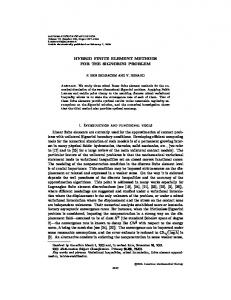
X2
q=0
u = 400
u = 300
analysis. However, in the formulation of BEM, the treatment of interface continuity conditions between adjacent subdomains can highly weaken the symmetry of the coefficient matrix of the final solving equation in the formulation of BEM. In this study, the hybrid finite element formulation with fundamental solution kernels (HFS-FEM) will be extended to the nonlinear heat conduction problems with temperaturedependent thermal conductivity, by coupling the noniteration technique, Kirchhoff transformation [18]. During the computation, the Kirchhoff transformation is firstly employed to remove the temperature dependence of thermal conductivity, and then a new linear system in terms of the introduced Kirchhoff variable can be obtained. Subsequently, the fundamental-solution-based hybrid finite element formulation is presented to solve this new linear system. Once the Kirchhoff variable distribution in the domain under consideration is determined, the inverse transformation can be available to derive the desired temperature distribution. A brief outline of the paper is arranged as follows: the mathematical models including the basic equations of heat conduction, the Kirchhoff transformation, and the hybrid finite element formulation are described in Section 2, and numerical results are presented and discussed in Section 3. Finally, conclusions are summarized in Section 4.
X1 q=0
Figure 1: Sketch of material nonlinearity in unit square domain.
2.2. Kirchhoff Transformation. Usually, for the case that the material property is dependent on the temperature, that is, 𝑘 = 𝑘(𝑇), necessary iteration procedures, for instance, Newton iteration, Nash iteration, Picard iteration, and so on, can be employed to perform linearization for such nonlinear problems. In the present work, a noniteration technology is employed by introducing the Kirchhoff transformation such as [18] d𝜙 = 𝑘 (𝑇) d𝑇
or 𝜙 = ∫ 𝑘 (𝑇) d𝑇,
(4)
where 𝜙 is a new quantity named as Kirchhoff variable, which is related to the sought temperature field 𝑇. Then, substituting (4) into (2), one obtains 𝑞𝑖 = −𝑘 (𝑇)
𝜕𝜙 𝜕𝑇 𝜕𝑇 𝜕𝜙 = −𝑘 (𝑇) =− . 𝜕𝑋𝑖 𝜕𝜙 𝜕𝑋𝑖 𝜕𝑋𝑖
(5)
As a result, the nonlinear governing equation (1) and boundary conditions (3) reduce to the following linear system consisting of the linear partial differential equation associated with the introduced Kirchhoff variable 𝜙: 𝜕2 𝜙 𝜕 2 𝜙 + =0 𝜕𝑋12 𝜕𝑋22
(6)
and the transformed boundary conditions 𝜙 = 𝜙 (𝑇) 𝜓≡−
𝜕𝜙 𝑛 =𝑞 𝜕𝑋𝑖 𝑖
on Γ1 on Γ2 .
(7)
In this paper, two types of material nonlinearities are considered.
Mathematical Problems in Engineering
3
D
C
D
C
E
E
A
A
B
Regular mesh
B
Irregular mesh
Arerr (u)
Figure 2: Investigation of sensitivity to mesh distortion.
0.25
2.2.2. Exponent-Type Thermal Conductivity. Consider the following:
0.2
𝑘 = 𝑘0 𝑒(𝛼+𝛽𝑇)
(11)
Integrating (11) by the Kirchhoff transformation (4) gives
0.15
𝜙=
0.1
𝑘0 (𝛼+𝛽𝑇) 𝑒 𝛽
(12)
from which the inverse manipulation produces 0.5
𝑇= 0
0
2
4
6
8
Regular mesh Irregular mesh
Figure 3: Effect of location of source point to numerical accuracy.
2.2.1. Power-Type Thermal Conductivity. Consider the following: 𝑛
(8)
with constants 𝑘0 , 𝛼, 𝛽, and 𝑛. Integrating (8) by the Kirchhoff transformation (4) gives 𝑘0 𝑛+1 𝜙= (𝛼 + 𝛽𝑇) 𝛽 (𝑛 + 1)
(9)
from which the inverse manipulation produces 𝑇=
[𝛽 (𝑛 + 1) 𝜙/𝑘0 ] 𝛽
1/(𝑛+1)
−𝛼
.
(13)
10
𝛾
𝑘 = 𝑘0 (𝛼 + 𝛽𝑇)
ln (𝛽𝜙/𝑘0 ) − 𝛼 . 𝛽
(10)
2.3. Hybrid Finite Element Formulation. Currently, the hybrid finite element with fundamental solution as trial function has been successfully formulated to solve the linear heat transfer problems using general or special elements. In this section, the HFS-FEM is applied to solve the new linear system consisting of (6) and (7) to determine the induced Kirchhoff variable. The overall computing domain is firstly discretized with some elements. For a typical element 𝑒, the weak integral functional can be written as follows [12, 13]: 𝜕𝜙 2 𝜕𝜙 2 1 ) +( ) ] dΩ Π𝑚𝑒 = − ∫ [( 2 Ω𝑒 𝜕𝑋1 𝜕𝑋2
(14)
− ∫ 𝜓𝜙̃ dΓ + ∫ 𝜓 (𝜙̃ − 𝜙) dΓ, Γ2𝑒
Γ𝑒
where 𝜙 and 𝜙̃ stand for independent element interior and boundary fields, respectively. Within the element 𝑒, the assumed element interior field 𝜙, also named as intraelement field, is usually approximated
4
Mathematical Problems in Engineering −100
400
380 n=2
360
340
n=1
−200 Heat flux q1
Temperature
n=3
n=1
n=2 −300 n=3
320
Linear −400
300 0
0.2
0.4
0.6
0.8
0.2
0.4
0.6
0.8
1
X1
X1
Exact HFS-FEM
Exact HFS-FEM
Figure 4: Variation of temperature along the line 𝑋2 = 0.5 with different power order 𝑛.
by the linear combination of the fundamental solution 𝜙∗ (x, x𝑠 ), that is, 𝜙 (x, x𝑠 ) = {N} {c𝑒 } ,
Figure 5: Variation of heat flux along the line 𝑋2 = 0.5 with different power order 𝑛.
Subsequently, applying the Gaussian divergence theorem to (14), we have the following formula:
(15)
1 Π𝑚𝑒 = − ∫ 𝜓𝜙 dΓ − ∫ 𝜓𝜙̃ dΓ + ∫ 𝜓𝜙̃ dΓ 2 Γ𝑒 Γ2𝑒 Γ𝑒
where ∗ ∗ ∗ {N} = {𝜙1 𝜙2 ⋅ ⋅ ⋅ 𝜙𝑁𝑠 } , T
{c𝑒 } = {𝑐1 𝑐2 ⋅ ⋅ ⋅ 𝑐𝑁𝑠 } ,
(16)
and x and x𝑠 are field point and source field, respectively. 𝑁𝑠 is the number of source points x𝑠 located outside the element domain, and 𝑐𝑖 presents unknown source intensity. In the paper, two different fundamental solutions are involved. One is the general fundamental solution associated with the problem without hole, and another is the special fundamental solution associated with the problem with circular hole. For completeness, we present, in the Appendix, the involved expressions of fundamental solutions. According to the physical definitions of fundamental solutions given in the Appendix, we can easily find that the linear combination of fundamental solutions with different source points can exactly satisfy the linear partial differential equation (6) and the specified interfacial condition along the circular hole. This feature is important to simplify the hybrid functional (14) by removing the domain integral in it. Besides, the independent frame field defined over the element boundary is constructed by ̃ {d𝑒 } , 𝜙̃ (x) = {N}
0
1
(17)
̃ represent the element nodal degree where {d𝑒 } and {N} of freedom (DOF) and conventional interpolating shape functions, respectively.
(18)
in which only element boundary integrals are included. The substitution of (15) and (17) into (18) finally yields 1 T T T Π𝑚𝑒 = − {c𝑒 } [H𝑒 ] {c𝑒 } − {d𝑒 } {g𝑒 } + {c𝑒 } [G𝑒 ] {d𝑒 } , 2 (19) where [H𝑒 ] = ∫ {Q}T {N} dΓ, Γ𝑒
̃ dΓ, [G𝑒 ] = ∫ {Q}T {N} Γ𝑒
(20)
T
̃ 𝜓dΓ {g𝑒 } = ∫ {N} Γ2𝑒
with 𝜕 {N} [ 𝜕𝑥1 ] 𝜕 {N} ] 𝑛 = − {𝑛1 𝑛2 } [ {Q} = − [ 𝜕 {N} ] . 𝜕𝑥𝑖 𝑖 [ 𝜕𝑥2 ]
(21)
Mathematical Problems in Engineering
5 −100
400
𝛽 = 0.1
−105 𝛽 = 0.05
360
𝛽 = 0.01
Heat flux q1
Temperature
380
340
−1010 𝛽 = 0.05 −1015
320
300
𝛽 = 0.01
0
0.2
0.4
0.6
0.8
1
−1020
𝛽 = 0.1
0
0.2
0.4
0.6
X1
0.8
1
X1
Exact HFS-FEM
Exact HFS-FEM
Figure 6: Variation of temperature along the line 𝑋2 = 0.5 with different coefficient 𝛽.
The stationary conditions of the functional Π𝑚𝑒 with respect to {c𝑒 } and {d𝑒 } produce
Figure 7: Variation of heat flux along the line 𝑋2 = 0.5 with different coefficient 𝛽.
For the case of power-type variation of the thermal conductivity with temperature, that is, 𝑘 = 𝑘0 (𝛼 + 𝛽𝑇)𝑛 , an analytical solution of the form 𝑇 = ( {[(𝛼 + 400𝛽)
[K𝑒 ] {d𝑒 } = {g𝑒 } , −1
{c𝑒 } = [H𝑒 ] [G𝑒 ] {d𝑒 }
(22)
in which the stiffness equation and the optional relationship between {c𝑒 } and {d𝑒 } are well established.
3. Numerical Examples In this section, some numerical examples are presented to illustrate the validity of the proposed hybrid finite element formulation with fundamental solution kernels. There are few nonlinear problems that have the known exact solutions. Among them is the first example in Section 3.1. The numerical results computed by the present method are compared with the exact solutions. The second example in Section 3.2 is a problem with a centered circular cut, and the numerical results by the present algorithm are compared with those by the MATLAB PDE Toolbox.
3.1. Nonlinear Heat Transfer in a Unit Square. As a first example, let us consider the numerical solutions for plane heat transfer over a unit square domain. The temperatures on the left and right edges of the square remain 300 K and 400 K, respectively, while the remainders are assumed to be insulated, as shown in Figure 1.
𝑛+1
+(𝛼 + 300𝛽)
− (𝛼 + 300𝛽)
𝑛+1 1/(𝑛+1)
}
𝑛+1
] 𝑋1 −1
(23)
− 𝛼) (𝛽)
is obtained to verify the numerical solutions. In the practical computation, two different mesh schemes (regular mesh and irregular mesh) are employed to model the square domain and validate the stability of the proposed approach (see Figure 2). For this purpose, we first set 𝑘0 = 1, 𝑛 = 1, 𝛼 = −2, and 𝛽 = 0.01, which corresponds to 𝑘 = −2 + 0.01𝑇 and 𝑇 = 100√3𝑋1 + 1 + 200. Figure 3 displays the variation of the error defined by 2
Arerr (𝑢) = √
∑𝑁 𝑖=1 (𝑢HFS-FEM − 𝑢exact )𝑖 2
∑𝑁 𝑖=1 (𝑢exact )𝑖
(24)
with the parameter 𝛾, which controls the location of source point used for intraelement approximation. It can be seen that there are large stable range to choose the parameter 𝛾, for either regular or irregular meshes. At the same time, one also observes that too small values of 𝛾, meaning that the source points lie so closely to the element boundary that the distance 𝑟 between the source points and element nodes approaches to zero, bring bad results. The main reason is that the kernel functions of the fundamental solution vary according to 𝑂(ln 𝑟), and 𝑂(𝑟−2 ), respectively, in two dimensions so that inaccuracies in the evaluation of element boundary integrals (near-singular problems) would be caused when 𝑟 approaches to zero. On the other hand, too large value of 𝛾 corresponding to the large distance of the source points and element nodes
6
Mathematical Problems in Engineering Table 1: Sensitivity to distortion of sub-domain mesh. Regular mesh 324.9997 374.9998 339.1944 385.4052 358.1139 Regular mesh −150.0053 −150.0053 −150.0053 −150.0053 −149.9287
A B C D E A B C D E
Irregular mesh 324.9990 375.0006 339.1934 385.4057 358.1139 Irregular mesh −150.0102 −150.0034 −150.0033 −150.0103 −149.8496
will affect the inverse manipulation of the element matrix {H𝑒 }, which is nearly singular due to the almost same entries [12]. Therefore, 𝛾 = 5 is chosen in the following practical computation. To investigate the sensitivity to mesh distortion of the presented formulation, numerical results at five test points for uniform and distorted meshes are obtained by the formulation presented in the paper and displayed in Table 1. The coordinates of the five test points are, respectively, A(0.1875, 0.2500), B(0.6875, 0.2500), C(0.3125, 0.7500), D(0.8125, 0.7500), and E(0.5000, 0.5000). As expected, a marked insensitivity to the mesh distortion is observed in the table. Besides, we find that the results inside the subdomains, that is, at points A, B, C, and D, are less affected by the irregularity of the mesh than those at the subdomains boundary point E. Next, the temperature and heat flux distributions with various power parameter 𝑛 are, respectively, given in Figures 4 and 5 to illustrate the effect of nonlinear material property. It can be seen that the temperature profile becomes steeper, and the temperature gradient has larger value, as 𝑛 increases. Besides, the good agreement between numerical results and exact solutions means that the proposed approach can capture the nonlinear effect, even with coarse mesh. In contrast to the power-type variation of thermal conductivity, another form of thermal conductivity with exponent expression is also investigated in this example. For the case 𝑘 = 𝑘0 𝑒(𝛼+𝛽𝑇) , it is easy to get the following analytical solutions: 𝑇=
ln [(𝑒𝛼+400𝛽 − 𝑒𝛼+300𝛽 ) 𝑋1 + 𝑒𝛼+300𝛽 ] − 𝛼 𝛽 𝑞1 = −
,
𝑘0 (𝛼+400𝛽) (𝛼+300𝛽) −𝑒 ]. [𝑒 𝛽 (25)
During computation, the same 2 by 2 regular mesh as the one used in the previous test is used to model the computing domain. Simultaneously, we keep 𝑘0 = 1 and 𝛼 = −2 invariant. The results obtained by the HFS-FEM are displayed in Figures 6 and 7, from which we notice that the results of HFS-FEM and exact solutions agree well. At the same
(|𝑇regular − 𝑇irregular |/|𝑇regular |) × 100% 0.000 0.000 0.000 0.000 0.000 (|𝑞1regular − 𝑞1irregular |/|𝑞1regular |) × 100% 0.003 0.001 0.001 0.003 0.053
time, it is found that the temperature curve shows stronger nonlinearity, as the parameter 𝛽 becomes larger. Meanwhile, the average values of heat flux component 𝑞1 dramatically increase by almost fourteen orders of magnitude, that is, the value increases from −466.9718 to −3.1847 × 10¹⁷ . 3.2. Nonlinear Heat Transfer in a Unit Square with a Circular Cut. To illustrate the advantage of the present approach over the conventional FEM in the aspect of mesh reduction, let us consider a unit square with a centered circular cut. The diameter of the circular hole is taken to be 0.5. The boundary conditions along the outer edges of the square are the same as those in the previous example, and the rim of the hole is assumed to be insulated. The thermal conductivity of the material is assumed as 𝑘 = −2 + 0.01𝑇. In the computation, two special elements, respectively, including 8 nodes and 16 nodes are compared (see Figure 8) to investigate the change of accuracy of the present algorithm. Figure 9 displays the temperature isoline maps corresponding to the two different elements shown in Figure 8. In the figure, the numerical results of conventional FEM implemented by MATLAB PDE toolbox are also provided to make comparison. Total 4448 triangle finite elements with 2339 nodes are employed to discretize the computing domain in the MATLAB PDE toolbox. It can be observed that the numerical accuracy of the present special elements increases, as the number of nodes of the special element becomes large. Moreover, there is a good agreement between the numerical results of the present special element with 16 nodes and that of MATLAB PDE toolbox. More interestingly, a great effect on mesh reduction is achieved by use of the proposed special elements. Thus, the present hybrid finite element model with special elements can obtain better efficiency than the conventional FEM, when the circular hole exists in the computing domain.
4. Conclusions The present study proposes the fundamental-solution-based hybrid finite element formulation to solve the nonlinear heat
Mathematical Problems in Engineering
7
(a) 8-node special circular hole element
(b) 16-node special circular hole element
Figure 8: Two special elements with different number of nodes.
395
385
390
0.8 395
0.8
305 310 315 320 325 330 335 340 345 350 355 360 365 370 375 380
1
305 310 315 320 325 330 335 340 345 350 355 360 365 370 375 380 385 390
1
X2
0.6
X2
0.6
0.4
0.4
0.2
0.2
0
0
0.2
0.4
0.6
0.8
1
0
0
0.2
0.4
X1
0.6
0.8
1
X1
MATLAB 8-node element
MATLAB 16-node element
Figure 9: Temperature distribution in the computing domain.
conduction problems with temperature-dependent thermal conductivity. It is a direct extension of the HFS-FEM for linear heat conduction problems by combining the Kirchhoff transformation and it is easy to be numerically implemented. The numerical results show that the present hybrid finite element formulation is very effective and convenient to solve the nonlinear heat conduction problem. It is shown that, for the analysis of nonlinear heat conduction problems, especially those related to the circular hole, the improvements of both the efficiency of mesh discretization and the numerical
accuracy of the present hybrid finite element model are significant, for the sake of the use of general or special fundamental solutions.
Appendix Fundamental Solutions In the formulation of the present hybrid finite element, the fundamental solution of the problem plays an important
8
Mathematical Problems in Engineering
role. Based on the mathematical definition of them, they are employed to construct the element interior field, which exactly satisfies the governing equation, and simultaneously convert the domain integral into the boundary integral in the hybrid functional. General Fundamental Solution. For the general case without holes in the 2D infinite plane, the fundamental solution 𝜙∗ (x, x𝑠 ) of the problem is required to satisfy the following partial differential equation: (
𝜕2 𝜕2 + 2 ) 𝜙∗ (x, x𝑠 ) + 𝛿 (x, x𝑠 ) = 0 ∀ x, x𝑠 ∈ R2 2 𝜕𝑥1 𝜕𝑥2 (A.1)
which produces 𝜙∗ (x, x𝑠 ) = −
1 Re [ln (𝑧 − 𝑧𝑠𝑗 )] . 2𝜋
(A.2)
In (A.1) and (A.2), 𝛿 represents the Dirac delta function, Re denotes the real part of the bracketed expression, and 𝑧 = 𝑠 𝑠 + 𝑥2𝑗 𝑖 are the field point and source 𝑥1 + 𝑥2 𝑖 and 𝑧𝑠𝑗 = 𝑥1𝑗 point expressed in the complex space, respectively. The derivative of (A.2) is given by 𝜕𝜙∗ 1 1 ]. = − Re [ 𝜕𝑧 2𝜋 𝑧 − 𝑧𝑠𝑗
(A.3)
Special Fundamental Solution. Specially, when there is a central circular hole with radius 𝑅 in the 2D infinite plane, the fundamental solution satisfies both partial differential equation (A.1) and the specific boundary condition along the rim of circular hole. Here, the insulated boundary condition 𝜕𝜙∗ /𝜕𝑛 = 0 is assumed, and the corresponding special fundamental solutions can be written as 𝜙∗ (𝑧, 𝑧𝑠𝑗 ) = −
(𝑧 − 𝑧𝑠𝑗 ) (𝑅2 − 𝑧𝑧𝑠𝑗 ) 1 Re [ln ] 2𝜋 𝑧
(A.4)
whose derivative is 𝑧𝑠𝑗 𝑅2 − 𝑧2 𝑧𝑠𝑗 𝜕𝜙∗ 1 = − Re [ ]. 𝜕𝑧 2𝜋 𝑧 (𝑧 − 𝑧𝑠𝑗 ) (𝑅2 − 𝑧𝑧𝑠𝑗 )
(A.5)
Acknowledgments This research work was partially supported by the Natural Science Foundation of China under Grant nos. 11102059 and 51178165. This financial support is gratefully acknowledged. Also, the authors would like to thank the support of the basic research programs from Henan Province Office of Education and Henan University of Technology.
References [1] K. J. Bathe and M. R. Khoshgoftaar, “Finite element formulation and solution of nonlinear heat transfer,” Nuclear Engineering and Design, vol. 51, no. 3, pp. 389–401, 1979.
[2] M. Kˇr´ızˇek and L. Liu, “Finite element approximation of a nonlinear heat conduction problem in anisotropic media,” Computer Methods in Applied Mechanics and Engineering, vol. 157, no. 3-4, pp. 387–397, 1998. [3] D. Lesnic, L. Elliott, and D. B. Ingham, “Identification of the thermal conductivity and heat capacity in unsteady nonlinear heat conduction problems using the boundary element method,” Journal of Computational Physics, vol. 126, no. 2, pp. 410–420, 1996. [4] T. Goto and M. Suzuki, “A boundary integral equation method for nonlinear heat conduction problems with temperaturedependent material properties,” International Journal of Heat and Mass Transfer, vol. 39, no. 4, pp. 823–830, 1996. [5] M. I. Azis and D. L. Clements, “Nonlinear transient heat conduction problems for a class of inhomogeneous anisotropic materials by BEM,” Engineering Analysis With Boundary Elements, vol. 32, no. 12, pp. 1054–1060, 2008. [6] M. Tanaka, T. Matsumoto, and S. Takakuwa, “Dual reciprocity BEM for time-stepping approach to the transient heat conduction problem in nonlinear materials,” Computer Methods in Applied Mechanics and Engineering, vol. 195, no. 37-40, pp. 4953–4961, 2006. [7] W. T. Ang and D. L. Clements, “Nonlinear heat equation for nonhomogeneous anisotropic materials: a dual-reciprocity boundary element solution,” Numerical Methods for Partial Differential Equations, vol. 26, no. 4, pp. 771–784, 2010. [8] A. Karageorghis and D. Lesnic, “Steady-state nonlinear heat conduction in composite materials using the method of fundamental solutions,” Computer Methods in Applied Mechanics and Engineering, vol. 197, no. 33–40, pp. 3122–3137, 2008. [9] L. Marin and D. Lesnic, “The method of fundamental solutions for nonlinear functionally graded materials,” International Journal of Solids and Structures, vol. 44, no. 21, pp. 6878–6890, 2007. [10] Z. H. Gao, Y. M. Lai, M. Y. Zhang et al., “An element free Galerkin method for nonlinear heat transfer with phase change in Qinghai-Tibet railway embankment,” Cold Regions Science and Technology, vol. 48, no. 1, pp. 15–23, 2007. [11] A. Singh, I. V. Singh, and R. Prakash, “Meshless element free Galerkin method for unsteady nonlinear heat transfer problems,” International Journal of Heat and Mass Transfer, vol. 50, no. 5-6, pp. 1212–1219, 2007. [12] H. Wang and Q. H. Qin, “Hybrid FEM with fundamental solutions as trial functions for heat conduction simulation,” Acta Mechanica Solida Sinica, vol. 22, pp. 487–498, 2009. [13] H. Wang and Q. H. Qin, “Special fiber elements for thermal analysis of fiber-reinforced composites,” Engineering Computations, vol. 28, no. 8, pp. 1079–1097, 2011. [14] H. Wang and Q. H. Qin, “A fundamental solution-based finite element model for analyzing multi-layer skin burn injury,” Journal of Mechanics in Medicine and Biology, vol. 12, no. 5, Article ID 125002, 22 pages, 2012. [15] H. Wang and Q.-H. Qin, “Fundamental-solution-based hybrid FEM for plane elasticity with special elements,” Computational Mechanics, vol. 48, no. 5, pp. 515–528, 2011. [16] H. Wang and Q.-H. Qin, “Boundary integral based graded element for elastic analysis of 2D functionally graded plates,” European Journal of Mechanics, vol. 33, pp. 12–23, 2012. [17] H. Wang and Q.-H. Qin, “A new special element for stress concentration analysis of a plate with elliptical holes,” Acta Mechanica, vol. 223, no. 6, pp. 1323–1340, 2012. [18] L. M. Jiji, Heat Conduction, Springer, 2009.
Advances in
Operations Research Hindawi Publishing Corporation http://www.hindawi.com
Volume 2014
Advances in
Decision Sciences Hindawi Publishing Corporation http://www.hindawi.com
Volume 2014
Journal of
Applied Mathematics
Algebra
Hindawi Publishing Corporation http://www.hindawi.com
Hindawi Publishing Corporation http://www.hindawi.com
Volume 2014
Journal of
Probability and Statistics Volume 2014
The Scientific World Journal Hindawi Publishing Corporation http://www.hindawi.com
Hindawi Publishing Corporation http://www.hindawi.com
Volume 2014
International Journal of
Differential Equations Hindawi Publishing Corporation http://www.hindawi.com
Volume 2014
Volume 2014
Submit your manuscripts at http://www.hindawi.com International Journal of
Advances in
Combinatorics Hindawi Publishing Corporation http://www.hindawi.com
Mathematical Physics Hindawi Publishing Corporation http://www.hindawi.com
Volume 2014
Journal of
Complex Analysis Hindawi Publishing Corporation http://www.hindawi.com
Volume 2014
International Journal of Mathematics and Mathematical Sciences
Mathematical Problems in Engineering
Journal of
Mathematics Hindawi Publishing Corporation http://www.hindawi.com
Volume 2014
Hindawi Publishing Corporation http://www.hindawi.com
Volume 2014
Volume 2014
Hindawi Publishing Corporation http://www.hindawi.com
Volume 2014
Discrete Mathematics
Journal of
Volume 2014
Hindawi Publishing Corporation http://www.hindawi.com
Discrete Dynamics in Nature and Society
Journal of
Function Spaces Hindawi Publishing Corporation http://www.hindawi.com
Abstract and Applied Analysis
Volume 2014
Hindawi Publishing Corporation http://www.hindawi.com
Volume 2014
Hindawi Publishing Corporation http://www.hindawi.com
Volume 2014
International Journal of
Journal of
Stochastic Analysis
Optimization
Hindawi Publishing Corporation http://www.hindawi.com
Hindawi Publishing Corporation http://www.hindawi.com
Volume 2014
Volume 2014