FURS: Fast and Unique Representative Subset ... - FTP Directory Listing

Social Network Analysis and Mining manuscript No. (will be inserted by the editor)

FURS: Fast and Unique Representative Subset selection retaining large scale community structure Raghvendra Mall · Rocco Langone · Johan A.K. Suykens

the date of receipt and acceptance should be inserted later

Abstract We propose a novel algorithm, FURS (Fast and Unique Representative Subset selection) to deterministically select a set of nodes from a given graph which retains the underlying community structure. FURS greedily selects nodes with high-degree centrality from most or all the communities in the network. The nodes with high-degree centrality for each community are usually located at the center rather than the periphery and can better capture the community structure. The nodes are selected such that they are not isolated but can form disconnected components. The FURS is evaluated by means of quality measures like coverage, clustering coefficients, degree distributions and variation of information. Empirically, we observe that the nodes are selected such that most or all of the communities in the original network are retained. We compare our proposed technique with state-of-the-art methods like SlashBurn, Forest-Fire, Metropolis and Snowball Expansion sampling techniques. We evaluate FURS on several synthetic and real-world networks of varying size to demonstrate the high quality of our subset while preserving the community structure. The subset generated by the FURS method can be effectively utilized by model based approaches with out-of-sample extension properties for inferring community affiliation of the large scale networks. A consequence of FURS is that the Raghvendra Mall Department of Electrical Engineering, ESAT-SCD, Katholieke Universiteit Leuven, Kasteelpark Arenberg,10 B-3001 Leuven, Belgium Tel: +32 16/328657 E-mail: [email protected] Rocco Langone E-mail: [email protected] Johan A.K. Suykens E-mail: [email protected]

selected subset is also a good candidate set for simple diffusion model. We compare the spread of information over time using FURS for several real world networks with random node selection, hubs selection, spokes selection, high eigenvector centrality, high Pagerank, high betweenness centrality and low betweenness centrality based representative subset selection. Keywords Node subset selection · hubs · community detection · simple diffusion model

1 Introduction In the modern era graphs have become universal. Their applications span from social network analysis, bio-informatics, telecommunication networks to even software engineering. With the advancement of technology, widespread use of Internet and availability of cheap sensors, the amount of information that can be collected is only increasing. This leads to large scale graphs with hundreds of thousands to even millions of nodes. There are several internet based organizations from Facebook to LinkedIn which produces graphs ranging from online social networks to professional networks scaling to 100 million users [Crandall et al., 2008], [Ferrara, 2012], [Pham et al., 2011], [Leskovec et al., 2008] and captures the interactions between these users. In the telecommunication field, the cell phone interactions produces large scale graphs and provide insight that groups of people prefer to converse with which other groups of people [Blondel et al., 2008] and [Saravanan et al., 2011]. In biological systems, graphs are generated from interactions between various entities which reflect the associations between these entities. For example the interactions between neurons in the brain to associations be-

2

tween the proteins in food synthesis [Jeong et al., 2000] and [Bullmore and Sporns, 2009]. Real world graphs exhibit community structure where the nodes are densely connected within the community and sparsely connected between the communities. The problem of community detection has received a lot of attention in recent years [Danon et al., 2005], [Fortunato, 2009],[Clauset et al., 2004], [Girvan and Newman, 2002], [Langone et al., 2012], [Lancichinetti and Fortunato, 2009b], [Rosvall and Bergstrom, 2008] and [Gilbert et al., 2011]. These communities are of great importance as they help to shed light on behavior and functioning of the networks, like buyer or seller behavior during times of crisis. However, the modern day networks are extremely large and detecting communities from these networks can become impractical and intractable due to memory and time constraints. The question to ask then is how to overcome the challenge of scale of the networks and perform data analysis of these networks. One direction to proceed is to develop efficient algorithms which are fast, accurate, scalable [Rosvall and Bergstrom, 2008], [Blondel et al., 2008] and might use parallelization or distributed computing. The other approach which has been receiving some attention lately is the method of sampling. Sampling is conventionally done by a stochastic algorithm when one is interested in performing computations that are too expensive for the large graph. A sample of the network can be a set of nodes from the large graph along with their edges. Another sample can be a set of edges from the large graph along with the corresponding vertices. The simplest technique for obtaining such a sample would be to perform a random sampling. Random sampling has been studied extensively in various domains to provide insightful information, particularly, in the case of online social network analysis [Gjoka et al., 2010] and [Catanese et al., 2011]. However, the subgraph obtained by random sampling does not retain the inherent community structure. Thus, the sampling of the network should be performed such that the obtained subgraph is a good representative of the original network. But how does one measure if a subgraph is a ‘good representative’ of the larger network? Existing work using graph properties like degree distributions and clustering coefficients are [Hubler et al., 2008] and [Leskovec and Faloutsos, 2006]. Another work argues that the measure of representativeness varies and depends on the analysis to be performed [Maiya and Berger-Wolf, 2010]. In this paper, we use several evaluation metrics like Coverage (Cov), fraction of communities preserved (Frac), clustering-coefficients (CCF), degree distributions (DD) and variation of in-

Raghvendra Mall et al.

formation (VI) to determine the quality of the subset generated by FURS.

1.1 Motivation & Contributions Recent work [Gleich and Seshadhri, 2012] showed that egonets can exhibit conductance scores as good as the Fiedler cut and provide a good seed sample for a partitioning method like PageRank clustering. However, another work [Kang and Faloutsos, 2011] suggests that real world scale-free networks follow power-law degree distributions and have ‘no good cuts’. They provide an ordering of the nodes of the graph (SlashBurn algorithm) to obtain a good compression of the real world graphs. We concur with [Kang and Faloutsos, 2011] and observe that nodes with high degree centrality or hubs tend to be part of dense regions of a graph. The aim of this work is to select a subset of nodes which are located at the center of the communities in the large scale network without explicitly performing community detection. The nodes which are located at the center are good representative of the underlying community structure. The concept is parallel to the concept of identification and selection of k centroids for the k-means clustering technique [MacQueen, 1967]. For this purpose we want to locate and select nodes with high degree centrality. This is because nodes with high PageRank centrality [Katz, 1953, Bonacich, 1987], eigenvector centrality [Katz, 1953, Bonacich, 1987] and betweenness centrality [Freeman, 1979] can be influential nodes in the large scale network but need not necessarily be at the center of the communities. This problem of selection of a subset where the nodes are central to the communities present in the large network without explicitly perform community detection is NP-hard. We propose a Fast and Unique Representative Subset (FURS) selection technique which is a greedy approximation of the above criterion. The basic idea is to first order the nodes based on their degree in descending order during each iteration and pick the node with highest degree centrality. Once such a node is selected its immediate neighbors are deactivated (as they can be reached directly from this node) during that iteration and the node is placed in the selected subset without changing the graph topology. We then select the node with highest degree centrality among the active nodes and the process is repeated until we reach the subset size. Once all nodes are deactivated, a new iteration is started and the deactivated nodes are re-activated. They are ordered according to their degree centrality in descending order and the process of node selection, deactivation and reactivation is repeated till we obtain

FURS: Fast and Unique Representative Subset selection retaining large scale community structure

the desired subset. The proposed approach greedily selects nodes with high degree centrality from different dense regions of the graph. Thus, we propose a Fast and Unique Representative Subset (FURS) selection algorithm which deterministically obtains a representative subset of nodes while retaining the community structure of the large graph. The contributions of the paper are listed as the follows: – The sample set of nodes has high degree centrality. We observe that these nodes span the different communities in the graph capturing the community structure of the large network. This is evaluated by the metric fraction of communities of the large network preserved in the subset generated by the FURS. We experimentally demonstrate that the quality of the subset generated by FURS is better for several evaluation metrics than previous techniques. – We compare and show that the proposed subset selection technique is faster than the state-of-the-art sampling techniques like SlashBurn, Metropolis and Snowball Expansion sampling. – We show that the subset obtained by FURS is also a good candidate set for simple diffusion model. The spread of information over time using FURS is generally better than the candidate set obtained by random node selection, hubs selection, spokes selection, high eigenvector centrality, high Pagerank, high betweenness centrality and low betweenness centrality based representative subset selection. Related work in this domain is discussed in the next section. This is followed by the description of our proposed sampling technique in section 3. Section 4 explains the evaluation metrics and Section 5 illustrates the experiments conducted along with the analysis of the experiments. Section 6 reflects the applicability of FURS for inferring community affiliation in association with model based approach. Section 7 explains the usage of FURS as a candidate set for a simple diffusion model. We provide the conclusion in section 8. 2 Related Work Sampling techniques can be broadly divided into two categories: – Node sampling - Node sampling involves selecting nodes which form a representative subset of the graph. The selected set of nodes can either be connected or disconnected. The subgraph obtained from the subset containing disconnected nodes comprises disconnected components and can even have isolated nodes (w.r.t. the subgraph and not the large

3

scale network). Some node sampling techniques include randomly selecting nodes based on degree centrality, random walk model and forest-fire model [Leskovec and Faloutsos, 2006]. In [Leskovec and Faloutsos, 2006], they evaluate the quality of the samples for these methods based on their ability to match various properties of the original graph structure like degree distributions, clustering coefficients and component sizes. They conclude that the sample obtained by the forest-fire approach is better than other methods. We provide a brief description of the Forest-Fire model and the SlashBurn algorithm. 1. Forest-Fire - Firstly, a node is randomly picked as seed node. We then begin “burning” the outgoing links and the corresponding nodes. If a link gets burned, the node at the other endpoint gets a chance to burn its own links, and so on recursively. The Forest-Fire model has two parameters: forward (pf ) and backward (pb ) burning probability. 2. SlashBurn - Recently, a new approach was proposed to provide an ordering of the nodes of the graph namely SlashBurn algorithm. It was used to obtain a good compression of the real world graphs in [Kang and Faloutsos, 2011]. The SlashBurn algorithm can also be utilized for obtaining a subset of nodes which contain information about the inherent community structure. For the SlashBurn algorithm after selection of the k-hubset the connections are burnt and a new graph is constructed. The giant connected component is discovered in this new graph and the process of selection is performed recursively till we reach the required size of the subset. – Subgraph sampling - In subgraph sampling a new node is always selected from the neighborhood of an already selected node based on a criterion. As a result the obtained subgraph is always connected. This is a hard constraint and has to be followed making the problem more difficult and computationally expensive. In [Hubler et al., 2008], the Metropolis algorithm [Metropolis et al., 1953] was used for a sample subgraph selection. Recently, two sampling technique using the concepts of expander graph was published in [Maiya and Berger-Wolf, 2010] where the obtain subgraph is connected. We provide a brief description of Metropolis Sampling using Degree Distribution (MDD) [Metropolis et al., 1953] and Snowball Expansion Sampling (XSN) [Maiya and Berger-Wolf, 2010]. 1. Metropolis Sampling using Degree Distribution (MDD) - The idea behind MDD is to

4

Raghvendra Mall et al.

select a subgraph which has similar topological properties w.r.t. large graph. For MDD, the topological property is degree distribution. In order to get this subgraph, we draw a subgraph from the subgraph space following a specific density ρ(S). This density should reflect subgraph quality well, which means good induced subgraphs should be drawn more frequently than worse ones. Thus ρ(S) depends on the quality of subgraph G(S). It is not possible to draw samples from the sample space when the underlying normalized density ρ(S) is not known beforehand. To solve this problem we use the Metropolis algorithm [Metropolis et al., 1953]. 2. Snowball Expansion Sampling (XSN) - The XSN technique is based on the notion that samples with good expansion properties tend to be more representative of the community structure in the original network than samples with worse expansion. This concept is derived from the theories of expander graph. In Snowball Expansion Sampling the aim is to find a sample with max(S)| imum expansion factor i.e. |N|S| where N (S) is the neighbourhood of subgraph S. The term “snowball” is used because subsequent members of the sample (S) are selected from current neighbourhood set N (S) based on the degree to which a node v ∈ N (S) contributes to the expansion factor (|N ({v})−(N (S)∪S)|). New sample members can be chosen either deterministically or probabilistically and the process is continued till we reach the desired subgraph size. Thus, the sample grows as a snowball and results in a connected subgraph G(S). We compare our proposed algorithm with the ForestFire [Leskovec and Faloutsos, 2006] and SlashBurn [Kang and Faloutsos, 2011] techniques from Node Sampling methods. We also compare our approach with the Metropolis Sampling using Degree Distribution (MDD) [Metropolis et al., 1953] and Snowball Expansion Sampling (XSN) [Maiya and Berger-Wolf, 2010] which is better of the two methods that had been proposed in [Maiya and Berger-Wolf, 2010], from the Subgraph sampling methods. There have been other contributions involving sampling graphs for purposes like visualization [Rafiei, 2005], compression [Adler and Mitzenmacher, 2000], [Kang and Faloutsos, 2011],[Feder and Motwani, 1991], [Gilbert and Levchenko, 2004], sociology [Frank, 2005] and epidemiology [Goel and Salganik, 2009]. There is another work [Mehler and Skiena, 2009] which assumes that a network sample is already generated and contains nodes from a single community. With this assumption,

they propose a method to grow the network such that it includes all the members of this community. However, the aim of this paper is to come up with a fast technique to obtain a unique subset of nodes which represents all or most of the communities in the network. 3 Proposed Method We first provide a brief description of the notations which we will use throughout the paper.

3.1 Notions & Notations 1. A graph is mathematically represented as G = (V, E) where V represents the set of vertices or nodes and E ⊆ V × V represents the set of edges in a network. 2. The set S represents the subset of nodes obtained by the proposed technique such that S ⊂ V . 3. The subgraph generated by the subset of nodes S is represented as G(S). It can mathematically be depicted as G = (S, Q) where S ⊂ V and Q = (S × S) ∩ E represents the set of edges in the subgraph. 4. The subgraph G(S) can have disconnected components and the cardinality of the set S is given by s. 5. The degree distribution function is given by D(V ). 6. The adjacency matrix is denoted as A and the adjacency list corresponding to each vertex vi ∈ V is given by A(vi ). 7. The neighboring nodes of a given node vi are represented by N (vi ). 8. The median degree centrality of the graph is represented as M . 9. The cardinality of the set V is represented as n. 10. The cardinality of the set E is represented as e. All the graphs considered in this paper are assumed to be undirected and unweighted unless otherwise mentioned.

3.2 Core Concept Nodes which have a high degree centrality or hubs represent the existence of more interaction in the network and have the tendency of being located at the center of a community. However, it is essential to select several such nodes of high degree centrality from the different communities in the large network. But this problem of selection of such a subset S without explicitly performing community detection is NP-hard. Mathematically

FURS: Fast and Unique Representative Subset selection retaining large scale community structure

it can be formulated as: max S

s.t.

J(S) =

s X

D(vj )

j=1

(1)

vj ∈ c i , ci ∈ {c1 , . . . , ck }

where D(vj ) represents the degree centrality of the node vj , s is the size of the subset, ci represents the ith community and k represents the number of communities in the network which cannot be obtained explicitly. A greedy solution to the problem can be formulated in an optimization framework by maximizing the sum of the degree centrality of the nodes in selected subset S such that the neighbors of the selected nodes are deactivated for that iteration. By deactivating the neighbors we move from one dense region of the network to another dense region thereby approximately covering most or all the communities in the network. Till the subset size s is achieved, the deactivated nodes are activated in the next iteration and the procedure is reperformed. Algorithmically, it can be represented as, J(S) = 0 While |S| < s t

max S

s.t.

J(S) := J(S) +

s X

D(vj )

j=1

N (vj ) → deactivated, iteration t, N (vj ) → activated, iteration t+1, (2)

where st is the size of the set of nodes selected by FURS during iteration t.

3.3 FURS Procedure The FURS algorithm can be divided into three steps namely Hub Selection, Deactivation and Reactivation of nodes. We describe the FURS procedure in detail below: 1. Hub Selection - We first sort all the nodes on the basis of their degree centrality in descending order. We maintain the identity of the node and its corresponding degree centrality in a list. An important observation is that if two nodes have the same degree centrality, then after sorting they are maintained in an order which remains constant. Thus no matter how many times one runs the sorting procedure the nodes after sorting are always maintained in the same order. For example, consider a network

5

of 5 nodes ((v1 , 5), (v2 , 3), (v3 , 5), (v4 , 4), (v5 , 3)) where the first term in each tuple represents the node identifier and the second term represents the corresponding degree centrality. After sorting, the list is always represented as ((v1 , 5), (v3 , 5), (v4 , 4), (v2 , 3), (v5 , 3)). The technique for subset selection is inspired by the greedy algorithm used for maximum coverage problem in graphs as introduced in [Feige, 1998]. Before subset selection, we remove all the nodes from the graph whose degree centrality is less than the minimum of a user-defined threshold t and median degree centrality M of the network i.e. D(vi ) < min(t, M ) as we wish to select nodes of higher degree centrality and prevent the selection of outliers. By putting this condition, we remove all cliques of size min(t, M ) and discard such cliques as outlier community w.r.t. the size of other communities in the network. However, their connection with corresponding nodes is retained i.e. the degree distribution of the graph is retained. The median degree centrality M is the median value in the list of degree centrality values of all the nodes and is not affected by outliers. So, we prefer to use the median degree centrality instead of the mean degree centrality which is heavily influenced by outliers. After removal of all the nodes with degree centrality D(vi ) < min(t, M ), we pop the node with highest degree centrality from the list and select it as the new node say vj . 2. Deactivation - All the neighbors of vj obtained by A(vj ) are deactivated from the maintained list. By deactivating these nodes N (vj ), we simply don’t consider these nodes for selection for the time being without affecting the graph topology. Thus, the degree distribution of the remaining nodes V \(N (vj )∪ vj ) stays unaffected. We then select the node with the next highest degree centrality from the list say vp after deactivating the neighbors of vj and we deactivate N (vp ). By performing this operation, we ensure that the newly selected node will not appear in the neighbors of the existing subset of nodes for that iteration. This enables us to select nodes from different dense regions of the graph and thus have a representative subset containing nodes from most or all of the communities in the large network. 3. Reactivation - This process of selection of a node based on degree centrality and deactivating its immediate neighbors is performed iteratively until we obtain the required number of nodes which is equivalent to the subset size s. We observe empirically from our experiments that generally, it requires 2 iterations to obtain the required subset S.

6

Raghvendra Mall et al.

We sort these nodes based on their degree centrality, maintain a list and iteratively re-perform all the operations. By performing this operation, we end up selecting several nodes from each dense region of the graph. The subgraph obtained from the subset selected by FURS can have disconnected components. We put the constraint that the resulting subgraph G(S) does not contain isolated nodes as isolated nodes cannot capture underlying community structure. If the subgraph G(S) contains isolated nodes then the subset size s is increased iteratively to s := s + d0.05 × ne and FURS is re-performed. Thus nodes selected from each dense region are connected and the subset selected by FURS is not a maximal independent set of the large scale network. Algorithm 1 summarizes the FURS technique.

Algorithm 1: FURS Algorithm

1 2 3 4 5 6 7 8 9 10

11 12 13 14 15 16

Data: A list of nodes with their corresponding degree centrality values L = (V, D(V )), the median degree centrality M , user-defined threshold t, the adjacency matrix A with information about neighbors N (vi ), ∀vi ∈ V and cardinality of the set V i.e. n. Result: A subset of representative nodes S whose cardinality is s L := (V, D(V )), ∀vi ∈ V such that D(vi ) > min(t, M ) L := sort(L) // Based on the degree centrality values in descending order while |S| < s do // REACTIVATION Step if L == {} then L := L ∪ {vi , D(vi )}, ∀vi ∈ V that was deactivated. L := sort(L) // Based on the degree centrality values in descending order end // HUB SELECTION v1 := L.pop() // pop out the node with highest degree centrality S := S ∪ v1 // Add to output set S N b ← N (v1 ) // Neighboring nodes of v1 // Create a temporary list and add N b along with their corresponding degree centrality, if N (v1 ) is not already present in the list. // DEACTIVATION Step L := L.deactivate(N b, D(N b)) // Deactivate the neighbors of v1 end if ∼ isempty(Isolated Nodes(S)) then s := s + d0.05 × ne. Re-perform FURS. end

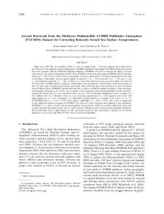
In Figure 1 the active nodes are always represented in darker shades and the deactivated nodes are represented in lighter shades. The selected nodes are always coloured in purple. Figure 1 explains the working mech-

anism of FURS selection procedure on a small network of 18 nodes. FURS selects 6 nodes from this network and the subgraph corresponding to this subset contains nodes from all the communities in the network. We observe from Figure 1 the presence of 3 cliques C1, C2 and C3 of size 5, 6 and 7 respectively with few interconnections between them. We calculate the degree centrality values and maintain a sorted list L of the node identifier and the degree centrality of the corresponding node. Here, L = {(v18 , 7), (v17 , 7), (v16 , 6), (v15 , 6), (v14 , 6), (v13 , 6), (v12 , 6), (v1 , 6), (v4 , 6), (v3 , 5), (v2 , 5), (v6 , 5), (v5 ,5), (v11 , 5), (v8 , 5), (v9 , 4), (v10 , 4), (v7 , 4)}. In Figure 1a, we select the 1st node or the node with the highest degree centrality i.e. v18 and deactivate all the nodes of clique C3 along with node v11 which are neighbors of node v18 . After that we select node v1 whose degree centrality 6 is maximum among the activated nodes. We deactivate all the nodes of clique C2 and node v8 which are neighbors of v1 . This is depicted in Figure 1b. We then select v9 which has maximum degree centrality (D(v9 ) = 4) among the currently activated nodes. We observe that all the other nodes in the network are deactivated as observed in Figure 1c. We then remove all the selected nodes and reactivate all the previously deactivated nodes. Then, list L = {(v17 , 7), (v16 , 6), (v15 , 6), (v14 , 6), (v13 , 6), (v12 , 6), (v4 , 6), (v3 , 5), (v2 , 5), (v6 , 5), (v5 , 5), (v11 , 5), (v8 , 5), (v10 , 4), (v7 , 4)}. Since the required subset size (s = 6) is not equal to the current subset size (s1 = 3 i.e. the size of subset after iteration 1 is 3), so we activate all the deactivated nodes. We then select node v17 whose degree centrality is 7. It is followed by deactivating all the nodes in clique C3 and node v4 which are immediate neighbors of the node v17 . This step is depicted in Figure 1d. Figure 1e shows the selection of node v3 from clique C2 as it has maximum degree centrality among the activated nodes. Finally, Figure 1f highlights the selection of node v11 as D(v11 ) = 5. The resulting subgraph is shown in Figure 1g and contains a disconnected component corresponding to clique C2. Thus the resulting subgraph G(S) captures community information about all the three communities present in the network. 3.4 Time Complexity The FURS algorithm results in a unique representative subset of the entire network as the selection process is deterministic. The initial seed node is selected such that it has the highest degree centrality in the graph. In order to maintain the list L of nodes along with their corresponding degree centrality in the ranking of largest to smallest degree centrality value, we need to sort L. This

FURS: Fast and Unique Representative Subset selection retaining large scale community structure

(b) Select node v1 with highest (a) Select node v18 with highest de- degree 6 among active nodes in gree 7 in L and deactivate its neigh- L and deactivate its neighbours bours (v17 , v16 , v15 , v14 , v13 , v12 , v11 ). (v4 , v3 , v2 , v6 , v5 , v8 ).

(c) Select node v9 with highest degree 4 among active nodes in L and deactivate its neighbours (v10 , v7 ). There are no more active nodes in L. Removing the selected nodes all the deactivated nodes are reactivated.

(f) Finally select node v11 with the highest degree 5 among the active (d) Select node v17 with highest de- (e) Select node v3 with highest degree nodes in L and deactivate its neighgree 7 in L and deactivate its neigh- 6 among the active nodes in L and de- bours (v8 , v10 , v7 ). There are again no more active nodes but we have bours (v16 , v15 , v14 , v13 , v12 , v4 ). activate its neighbours (v2 , v6 , v5 ). reached the desired subset size and stop FURS here.

(g) FURS Subgraph - Retains the inherent community structure with nodes from each clique (C1, C2,C3).

Fig. 1: Steps involved in FURS for a subset of size 6 from a network of 18 nodes.

7

8

is computationally the most expensive step of our proposed algorithm. The minimum time required to perform this sorting is O(n. log(n)). Every time L becomes empty, we reinitialize the list L with the nodes and degree centrality values of the nodes which were deactivated in the previous iteration. Let the number of such iterations required be iter. Thus, the overall computations required for sorting becomes O(iter.n. log(n)). In general, we observe that 2-3 iterations are sufficient to obtain the required subset S. Apart from sorting the list L, the other computation that is being performed is deactivating the neighbors of the winning node. Let S = (p1 , p2 , . . . , ps ) be the set of nodes sampled by the proposed algorithm. For each node pi ∈ S, we have to deactivate all its neighbors N (pi ). Deactivating each neighbor of a node pi takes unit computation time. The computational time required for the purpose of deactivation can then be Ps represented as O( i=1 N (pi )). Thus, the overall computational complexity of the algorithm is O(iter.n. log(n) Ps + i=1 N (pi )).

4 Evaluation Metrics Current community detection algorithms generate different partitions in each iteration for a given large scale network. For a fair comparison, we first generate a partition of the large graph using a scalable community detection algorithm and then run the same algorithm on the subgraphs generated by various sampling techniques. In order to obtain method-independent results we experimented with three different community detection algorithms namely CNM [Clauset et al., 2004], Infomap [Rosvall and Bergstrom, 2008] and Louvain [Blondel et al., 2008] as these approaches can handle large scale networks. We then evaluate the subgraph generated by each selection technique on various metrics like time required to generate the subgraph, clustering coefficients, degree distributions, coverage, variation of information and fraction of communities preserved. The results reported are the mean values for the various evaluation metrics. The measures like variation of information, clustering coefficients, degree distribution compare the extent of similarity of the generated subgraph G(S) with respect to the subgraph for the same set of nodes in the original graph G(S 0 ). A summary of the various evaluation metrics is mentioned below. Variation of Information: Variation of Information (VI) is an information theoretic measure and is used to compare two different partitions as depicted in

Raghvendra Mall et al.

[Meila, 2007]. Mathematically VI can be formulated as: V I(U, V ) =

k X r X nij i=1 j=1

n

log(

ni .nj /n2 ), nij /n2

where ni represents the number of nodes in cluster i in partitioning U and nj represents the number of nodes in cluster j in partitioning V and nij is the joint distribution of the cluster memberships in U and V . The VI measure is not normalized but it is bounded between the range [0; 2 log(max(k; r))] [Wu et al., 2009] where k is the number of clusters in one partition and r is the number of clusters in another partition. Lower values of VI means less variation between the two cluster membership lists and a value of 0 means perfect match between two cluster partitions. Hence, lower values of VI can be interpreted as less variation of information between the partitions. However, there exists other information theoretic measures like Normalized Mutual Information (NMI) [Lancichinetti et al., 2009] and Adjusted Rand Index (ARI) [Rabbany et al., 2012] which are normalized criterion and provide better interpretation. However, there is no one best information theoretic criteria for evaluating cluster memberships [Rabbany et al., 2012]. In our experiments we use variation of information (VI) criteria. Clustering Coefficient: The clustering coefficient (CCF) is defined as a vector with values ranging between [0, 1] both inclusive. We compare it using the L1 -norm. In order to prevent any bias like a single degree dominating the distance, we prevent the use of higher order L-norms including L∞ . We calculate the average (absolute) difference between the clustering P coefficients which is mathematically formulated as v∈S

|G(v)−S(v)|

. Once we obtain this average distance, |S| we convert it into similarity measure by subtracting the distance from 1 as in [Maiya and Berger-Wolf, 2010]. Degree Distribution: We compare the degree distributions (DD) of the large graph and the subgraph generated by the selection technique using the KolmogorovSmirnov D-Statistics as employed in [Hubler et al., 2008], [Maiya and Berger-Wolf, 2010].The Kolmogorov-Smirnov D-Statistics corresponds to the maximum difference between the two cumulative distribution functions FY of G and FY 0 of S over the range of random variables Y and Y 0 . Y and Y 0 are distributed according to G and S respectively. The distance D(G, S) is formulated as: D(G, S) = maxv∈S |FY (v) − FY 0 (v)|. We convert this distance into a similarity measure by subtracting the distance from 1 as in [Maiya and Berger-Wolf, 2010]. Coverage: Coverage (Cov) is a simple evaluation metric which is defined as the ratio of the total number of unique nodes directly reachable from the nodes in

FURS: Fast and Unique Representative Subset selection retaining large scale community structure

the selected subset to the total number of nodes in the graph. It can be represented as the ratio of cardinality of the set of all the nodes directly reachable from the nodes in the selected subset to the total number of nodes in the graph and mathematically be formulated |∪ N (s )| as si ∈Sn i . Coverage varies between 0 and 1 and higher values result in better coverage. Fraction of Communities: We determine the fraction of total communities in the larger network represented by the subgraph generated by the selection technique as the fraction of communities preserved (Frac). This number ranges between 0 and 1 and was also used in [Maiya and Berger-Wolf, 2010].

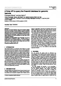
5 Experiments 5.1 Synthetic Networks We compare our proposed FURS selection technique with SlashBurn and Forest-Fire node sampling methods on a variety of synthetic networks of varying size and using different mixing parameters as depicted in Figure 2. These synthetic networks were generated by the software provided by Fortunato as mentioned in [Lancichinetti and Fortunato, 2009a]. We maintain the size of the subset as 15% of the nodes in the network based on experimental findings in [Leskovec and Faloutsos, 2006] and set the k values for k-hubset for SlashBurn as 0.5% of the nodes as per the recommendation in [Kang and Faloutsos, 2011]. From Figure 2, we observe that Forest-Fire (FF) node sampling is a fast subset selection technique but doesn’t retain the original community structure as can be observed from the VI for Louvain and Infomap method and also the fraction of communities preserved for Louvain method. For the FF method the forward pf and backward pb burning probability are set to pf = 0.7 and pb = 0.3 as given in [Leskovec and Faloutsos, 2006]. The Cov value turns out to be high for FF sampling except for synthetic networks with 5, 000 nodes. The SlashBurn algorithm is computationally more expensive and doesn’t retain the CCF as well as FURS and Forest-Fire sampling techniques. However, the SlashBurn approach is quite consistent w.r.t. other evaluation metrics. The FURS selection technique is computationally least expensive and better retains the CCF. With the exception of synthetic networks with 5, 000 nodes the FURS technique preserves the community structure of larger networks even with high mixing parameter as depicted in Figure 2. So, for large scale networks it is better to use the FURS selection technique.

9

5.2 Real World Networks We compare our proposed sampling technique on several real-world networks ranging from social networks, communication networks, citation networks, collaboration networks, web graphs, internet peer to peer networks to road networks. These networks are available at the http://snap.stanford.edu/data/index.html. Table 1 reflects a few keys statistics of each network. Network p2p Cond-mat HepPh Enron Epinions Web-Stanford roadCA Livejournal

Nodes 10,876 23,133 34,401 36,692 75,879 281,903 1,965,206 3,997,962

Edges 39,994 186,936 421,578 367,662 508,837 2,312,497 5,533,214 34,681,189

CCF 0.008 0.6334 0.1457 0.497 0.2283 0.619 0.0464 0.3538

Table 1: Nodes (V), Edges (E) and Clustering Coefficients (CCF) for each network

5.3 Experimental Setup We compare our proposed FURS method with ForestFire sampling (FF) [Leskovec and Faloutsos, 2006], MDD [Hubler et al., 2008], Snowball Expansion (XSN) sampling [Maiya and Berger-Wolf, 2010] and SlashBurn algorithm [Kang and Faloutsos, 2011]. These are the stateof-the-art techniques for sampling community structure. For MDD the produced samples try to mimic the degree distribution of the original network. In XSN, the sample set S is selected such that it maximizes the expansion (S)| factor: |N|S| and the concept behind SlashBurn algorithm was explained earlier. We perform all the experiments on a computer with 12 Gb RAM and 2.4 GHz Intel Xeon processor. We perform 5 randomizations of community detection algorithms (Louvain, Infomap, CNM) on the large network and for each randomization, we perform community detection on the subgraph generated by each of the subset selection method. Thus, we report mean and standard deviation values for the various evaluation metrics. The subset size is maintained as 15% of the nodes in the network as per the experimental analysis in [Leskovec and Faloutsos, 2006]. For the Metropolis algorithm based MDD, we perform 1, 000 iterations to produce each sample. 5.4 Experimental Results We perform exhaustive experiments on 8 benchmark real world networks using various evaluation metrics. It

10

Raghvendra Mall et al.

Fig. 2: Comparison of FURS, SlashBurn and Forest-Fire Node sampling techniques for various evaluation metrics on synthetic networks with 5, 000, 10, 000, 25, 000, 50, 000 nodes with mixing parameter varying from 0.1 to 0.5

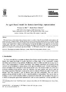
Fig. 3: Evaluation of various subset selection methods on 4 real world networks of increasing size is depicted in Table 2. Some of the abbreviated metrics in Table 2 are VI LN i.e. variation of information for Louvain method, Frac LN i.e. fraction of communities preserved by Louvain method. Other abbreviations include (VI IP) for variation of information for Infomap method, (VI CNM) for variation of information for CNM method, (Frac IP) for fraction of communi-

ties captured by Infomap method and (Frac CNM) for fraction of communities captured by CNM. We observe that the FURS approach performs well with respect to computation time, clustering coefficients, coverage and fraction of communities preserved by Louvain and Infomap method for most of the networks. FURS is better than at least three other sampling methods on most

FURS: Fast and Unique Representative Subset selection retaining large scale community structure Technique Properties Time CCF DD F Coverage U VI LN R Frac LN S VI IP Frac IP VI CNM Frac CNM Time S CCF L DD A Coverage S VI LN H Frac LN B VI IP U Frac IP R VI CNM N Frac CNM Time CCF DD X Coverage S VI LN N Frac LN VI IP Frac IP VI CNM Frac CNM Time CCF DD Coverage M VI LN D Frac LN D VI IP Frac IP VI CNM Frac CNM F Time O CCF R DD E Coverage S VI LN T Frac LN F VI IP I Frac IP R VI CNM E Frac CNM

p2p Mean Std 0.45 0.0 0.995 0.0 0.5 0.0 0.78 0.0 5.0 0.06 0.125 0.01 2.66 0.02 0.4 0.0 4.57 0.0 0.72 0.0 1.61 0.0 0.99* 0.0 0.723 0.0 0.81 0.0 5.16* 0.07 0.223 0.015 4.07* 1.55 0.22* 0.12 4.62* 0.0 0.75 0.0 37.2 10.7 0.992 0.0 0.783 0.0 0.56 0.01 4.9 0.05 0.028 0.0 2.24 0.09 0.97 0.01 4.56 0.07 0.22 0.02 21.9 0.2 0.992 0.0 0.78 0.01 0.55 0.01 4.9 0.04 0.027 0.0 2.2 0.03 0.98 0.0 4.56 0.12 0.2 0.01 0.48 0.01 0.992 0.0 0.77 0.01 0.55 0.01 4.92 0.06 0.028 0.0 2.32 0.17 0.96 0.04 4.58 0.17 0.22 0.02

Cond-mat Mean Std 4.92 0.0 0.73 0.0 0.853 0.0 0.83 0.0 4.67* 0.1 0.33 0.0 3.22 0.1 0.32 0.0 3.53 0.0 0.78 0.0 5.18 0 0.86 0 0.64* 0 0.82 0 3.4 0.1 0.08* 0.0 2.20 0.02 0.07* 0.0 2.77 0.0 0.56 0.0 270.9 2.9 0.44 0.01 0.91 0.0 0.57 0.0 4.28 0.05 0.32 0.004 4.63 0.07 0.32 0.0 3.76 0.07 0.43 0.01 273.6 1.8 0.44 0.01 0.91 0.0 0.57 0.0 4.3 0.04 0.32 0.0 4.66 0.07 0.32 0.01 3.8 0.12 0.324 0.02 4.95 0.01 0.44 0.01 0.91 0.0 0.57 0.0 4.27 0.06 0.32 0.0 4.68 0.06 0.32 0.0 3.78 0.06 0.21 0.03

HepPh Mean Std 17.05 0.0 0.87 0.0 0.81 0 0.882 0 1.22 0.1 0.16 0.01 0.52 0.10 0.075 0.0 1.58 0.0 0.03* 0.0 31.2 0 0.86 0 0.63* 0 0.9 0 1.07 0.08 0.19 0.0 0.55 0.02 0.09 0.0 1.35 0 0.06 0 312.5 8.44 0.76 0.0 0.96 0.0 0.81 0.0 3.5 0.07 0.07 0.0 3.3 0.17 0.33 0.02 2.91 0.18 0.86 0.04 323.08 13.8 0.76 0.0 0.96 0.0 0.8 0.0 3.43 0.04 0.07 0.01 3.23 0.11 0.06 0.0 2.8 0.08 0.83 0.05 17.15 0.03 0.76 0.0 0.96 0.0 0.80 0.0 3.49 0.1 0.07 0.0 3.3 0.06 0.06 0.0 2.89 0.15 0.85 0.07

Enron Mean Std 14.01 0.0 0.85 0.0 0.8 0.0 0.875 0.0 2.18 0.06 0.15 0.003 0.68 0.04 0.11* 0.0 1.95 0.0 0.103 0.0 35.6 0 0.92 0 0.46* 0 0.84 0 1.86 0.3 0.036* 0.0 2.83 1.38 0.143 0.07 2.22 0 0.03* 0 355.4 16.13 0.56 0.007 0.7 0.0 0.46 0.02 4.23 0.13 0.37 0.018 5.03 0.21 0.32 0.0 2.68 0.18 0.21 0.011 358.7 15.4 0.56 0.01 0.7 0.01 0.44 0.014 4.27 0.06 0.36 0.01 5.15 0.23 0.32 0.008 2.64 0.04 0.22 0.008 14.1 0.05 0.6 0.01 0.7 0.0 0.46 0.02 4.17 0.123 0.38 0.019 4.93 0.24 0.33 0.014 2.64 0.115 0.22 0.014

Epinions Mean Std 19.0 0.0 0.87 0.0 0.83 0 0.66 0 3.66 0.05 0.84 0.13 5.06 2.19 0.03 0.0 3.45 0 0.17 0 115.16 0 0.95 0 0.56 0 0.81 0 2.37 0.22 0.14* 0.03 2.31 2.1 0.04 0.02 2.17 0 0.065* 0.0 1453.1 30.0 0.87 0.0 0.53 0.003 0.38 0.007 5.63 0.124 0.143 0.03 7.73 0.98 0.00 0.0 3.33 0.085 0.18 0.01 1487.4 44.0 0.87 0.002 0.53 0.003 0.37 0.005 5.66 0.05 0.142 0.03 7.8 0.85 0.0 0.0 3.4 0.05 0.18 0.02 20.1 0.07 0.87 0.0 0.53 0.0 0.38 0.01 5.63 0.08 0.144 0.03 8.4 0.05 0.0 0.0 3.5 0.16 0.18 0.0144

Web-Stanford Mean Std 35.862 0 0.77 0 0.86 0.0 0.92 0 1.7 0.03 0.6 0.03 1.82 0.03 0.42 0.0 641.4 0 0.74 0 0.55* 0 0.84 0 1.15 0.07 0.75 0.045 1.72 0.08 0.53 0.0 9225 1980 0.47 0.02 0.95 0.0 0.42 0.03 3.89 0.2 0.06 0.0 4.36 0.2 0.042 0.0 8608 273.7 0.45 0.016 0.95 0.0 0.39 0.03 4.1693 0.3 0.058 0.0 4.64 0.273 0.04 0.002 37.8 0.1 0.47 0.0 0.95 0.0 0.42 0.04 3.8 0.40 0.06 0.0 4.27 0.4 0.042 0.0 -

roadCA Mean Std 49.4 0 0.94 0 0.85 0 0.43 0 0.014 0.0 0.03 0.0 4251.2 0 0.95 0.0 0.87 0.0 0.07* 0 0.01 0 0.02 0 50.24 0.5 0.95 0.0 0.84 0.0 0.35 0.0 0.013 0.0 0.025 0.0 -

11 Livejournal Mean Std 499 0.0 0.9051 0.0 0.79 0.0 0.75 0.0 0.023 0.0 85596 0.0 0.77 0.0 0.68* 0.0 0.68 0.0 0.2 0.0 501 1.0 0.73 0.01 0.8 0.01 0.51 0.02 0.012 0.0 -

Table 2: Statistics of real world networks for various subset selection techniques. Here ‘-’ represents not calculated as computationally too expensive and ‘*’ represents the cases for which FURS & SlashBurn algorithms perform worst. of the networks. However, FURS performs worst for Cond-mat network w.r.t. the metric VI LN, HepPh network w.r.t. the metric Frac CNM and Enron network w.r.t. the quality metric Frac IP. However, the other sampling techniques are worse on one or more properties for each network. This is highlighted in Table 2 for the SlashBurn approach which is our primary competitor. The SlashBurn performs worst for CCF, DD, Coverage, VI LN, Frac LN, VI IP, Frac IP, VI CNM and Frac CNM for one or more network. The SlashBurn method performs the worst for the p2p network. However, in general it can better capture the evaluation metric - variation of information for the different community detection algorithms. Figure 3 refers to the application of various subset selection techniques on 4 real world networks of increasing scale. We observe that the XSN and MDD technique become computationally infeasible for the roadCA network. We observe that the FURS selection technique is fast, has high clustering coefficients, coverage, smaller variation of information and better preserves the frac-

tion of community in the large networks. However, the internet peer to peer network network (p2p) is an exception on which the XSN, MDD and Forest-Fire (FF) sampling perform better. From Figure 3, we observe that the SlashBurn algorithm can effectively capture the variation of information for the large web network of Stanford University (web-Stanford) w.r.t. both Louvain and Infomap community detection methods. The VI metric can be high even when the Frac values are high. This is because size of the partitions in the subgraphs is not necessarily uniform. Hence, higher entropy and higher VI value as observed in some cases for FURS. We cannot evaluate the VI metric for massive scale networks like roadCA and Livejournal as it is computationally very expensive. 6 Inferring Community Affiliation In this section we explain the usage of FURS selection technique for inferring community affiliation for the unseen nodes of the large scale network. For this purpose

12

Raghvendra Mall et al.

we show the applicability of FURS along with a model based clustering method namely Kernel Spectral Clustering (KSC) [Alzate and Suykens, 2010], [Langone et al., 2012] and [Mall and Langone, 2013].

6.1 Primal-Dual Kernel Spectral Clustering Framework The Kernel Spectral Clustering (KSC) method was first proposed in [Alzate and Suykens, 2010] and extended to complex networks in [Langone et al., 2012] and [Mall and Langone, 2013]. It is based on a weighted kernel PCA formulation and the model is built in a primaldual optimization framework. The model has a powerful out-of-sample extension property which allows to infer community affiliation for unseen nodes. In case of complex networks, the adjacency list of the nodes in the subset S selected by FURS are treated as data points i.e. A(vi ) = xi , ∀vi ∈ S. Given a dataset D = {xi }si=1 , xi ∈ Rn , the training data points are provided by the FURS selection technique. Here xi represents the ith training point and is equivalent to the adjacency list i.e. A(vi ) of the ith node in subset S. The training set is represented by Xtr . The number of data points in the training set is equivalent to the subset size s. Given D and the number of clusters k, the primal problem of the spectral clustering via weighted kernel PCA is formulated as in [Alzate and Suykens, 2010]: k−1

min w(l) ,e(l) ,bl

(l)

|

ei = w(l) φ(xi ) + bl , i = 1, . . . , s,

(4)

where we take φ(xi ) = xi for large scale networks, bl (l) are the bias terms, l = 1, . . . , k − 1. The projections ei represent the latent variables of a set of k − 1 binary (l) cluster indicators given by sign(ei ) which can be combined with the final groups using an encoding/decoding scheme. The decoding consists of comparing the binarized projections w.r.t. codewords in the codebook and assigning cluster membership based on minimal Hamming distance. The dual problem corresponding to this primal formulation is: −1 DΩ MD Ωα(l) = λl α(l) ,

(5)

where MD is the centering matrix which is defined as MD = Is − (

−1 (1s 1| s DΩ ) ). | −1 1s DΩ 1s

The α(l) are the dual variables

and the positive definite kernel function K : Rn ×Rn → R plays the role of similarity function. This dual problem is closely related to the random walk model as shown in [Alzate and Suykens, 2010].

k−1

1 X (l) | (l) 1 X (l) | −1 (l) w w − γl e DΩ e 2 2s (3) l=1 l=1

such that e(l) = Φw(l) + bl 1s , l = 1, . . . , k − 1, (l)

for large scale networks. Since we use adjacency list of a node as a data point, the FURS selection technique can result in isolated nodes. Nodes which are isolated in the subgraph obtained by FURS technique might have common neighbors with other nodes in the subset S w.r.t. the large scale network and thus will contribute positively in the similarity function. The clustering model is then represented by:

(l)

where e(l) = [e1 , . . . , es ]| are the projections onto the eigenspace, l = 1, . . . , k − 1 indicates the number of score variables required to encode the k clusters, −1 DΩ ∈ Rs×s is the inverse of the degree matrix associated to the kernel matrix Ω. For large scale networks, the dimensionality of a data point xi can be equal to n when the ith node is connected to all the other nodes in the network. φ : Rn → Rnh is a feature mapping from n dimensions to nh dimensions, where nh can be infinite dimensional. Φ is the s × nh feature matrix, Φ = [φ(x1 )| ; . . . ; φ(xs )| ] and γl ∈ R+ are the regularization constants. We note that s  N i.e. the number of points in the training set is much less than the total number of data points for the network. The kernel matrix Ω is obtained by calculating the similarity between each pair of data points in the training set. Each element of Ω, denoted as Ωij = K(xi , xj ) = φ(xi )| φ(xj ) is obtained for example by the normalized linear kernel

6.2 Out-of-Sample Extensions Model The projections e(l) define the cluster indicators for the training data. In the case of an unseen data point x, the predictive model becomes: e(l) (x) =

s X

(l)

αi K(x, xi ) + bl

(6)

i=1

This out-of-sample extension property allows kernel spectral clustering to be formulated in a learning framework with training, validation and test stages for better generalization. The validation stage is used to obtain the model parameters like the number of clusters k in the network. The data points corresponding to the validation set are selected using FURS.

6.3 Model Selection The original KSC formulation [Alzate and Suykens, 2010] works well assuming piece-wise constant eigenvectors and using the line structure of the projections of the

FURS: Fast and Unique Representative Subset selection retaining large scale community structure

validation points in the eigenspace. It uses an evaluation criterion called Balanced Line Fit (BLF) for model selection i.e. for selection of k for the normalized linear kernel function. However, this criterion works well only in case of well separated clusters. So, we use the Balanced Angular Fit (BAF) criterion proposed in [Mall and Langone, 2013] for cluster evaluation. This criterion works on the principle of angular similarity and is efficient when the clusters are either well separated or overlapping. The BAF criterion varies from [-1, 1] and higher values are better for a particular k.

6.4 Experimental Results on Synthetic Network We generated synthetic networks containing 100, 000 nodes with various values of mixing parameter (µ) using the software provided in [Lancichinetti and Fortunato, 2009a]. In Figure 4, we show the result corresponding to µ = 0.1. To show that FURS can be used effectively for inferring community affiliation of the unseen nodes, we generate subsets of different sizes containing 2, 500, 5, 000, 7, 500, 12, 500 and 15, 000 nodes using the FURS selection technique. From Figure 4, we observe that time required for sampling 2, 500 and 5, 000 nodes are nearly equal. Time for sampling 7, 500, 10, 000 and 12, 500 are on the same scale as well. It is maximum for 15, 000 nodes. Sorting the nodes in the descending order of degree is the most time consuming step. For smaller size samples all the nodes are not deactivated and one iteration is sufficient, while for larger samples two iterations are required and three iterations are essential for 15, 000 nodes. The coverage increases as expected with the increase of the subset size. The clustering coefficients and degree distributions are nearly consistent and so is the fraction of communities (Frac) spanned with respect to the larger network. As shown in Figure 4, Frac= 1, even for a subset size of 2, 500 nodes indicating the inherent community structure can be captured with 2.5% of the nodes in the network. It forms a subgraph G(S) containing mostly isolated nodes. The quality of the predicted cluster memberships is further validated by two evaluation metrics i.e. low values for VI and high values for Adjusted Rand Index (ARI) [Hubert and Arabie, 1985].

13

[Granovetter, 1978] and [Shelling, 1978]. Several mathematical models for diffusion emerged such as local interaction games [Blume, 1993, Ellison, 1993, Goyal, 1996, Morris, 2000], threshold models [Granovetter, 1978], [Shelling, 1978, Kempe et al., 2005] and cascade models [Liggett, 1985, Goldenberg et al., 2001].

7.1 FURS for Simple Diffusion model In this paper, we show the effect that the subset S selected by FURS has for a very simple diffusion model. We consider the cascade model where each individual has a single, probabilistic chance (set to 1) to activate each of the inactive nodes in its immediate neighborhood after becoming active itself. Further, we consider the case of the very simple independent cascade model, in which the probability that an individual is activated by a newly active neighbor is independent of the set of neighbors who have attempted to activate it in the past. Starting with an initial active set S, the process unfolds in a series of time steps. At each time ti , any node vj who has just become active may attempt to activate each inactive node vk for which vj ∈ N (vk ). We set the probability p(vj , vk ) = 1 i.e. vk becomes active at the next time step if it was inactive. Real world networks exhibit community like structure as shown in [Fortunato, 2009], [Danon et al., 2005], [Clauset et al., 2004],[Girvan and Newman, 2002], [Lancichinetti and Fortunato, 2009b], [Langone et al., 2012] and [Rosvall and Bergstrom, 2008]. If real world networks have community structure then the nodes which are located at the center of the communities (i.e. hubs for each community) are good candidate for influential nodes. When this set of nodes are targeted for spread of information over the network then over various time stamps the information spread by means of this set should be the fastest. Since we are targeting the hubs the coverage w.r.t. the entire graph should also be maximal. As we claim that FURS selection technique can select nodes with high degree centrality from different dense regions of the large scale network, it becomes a good candidate for testing the aforementioned hypothesis.

7.2 Experimental Setup 7 Simple Diffusion Model The first study of diffusion in social networks emerged in the middle of the 20th century [Ryan and Gross, 1943] and [Coleman et al., 1966]. However, formal mathematical models of diffusion were introduced much later in

We compare the subset S obtained by FURS with subsets obtained by random node selection, hubs selection, spokes selection, high eigenvector centrality (HighEigen) [Katz, 1953, Bonacich, 1987], high Pagerank [Katz, 1953, Bonacich, 1987], high betweenness (HighBtw) centrality and low betweenness (LowBtw) cen-

14

Raghvendra Mall et al.

Fig. 4: Inferring Community Affiliation for large scale network using FURS selection technique trality [Freeman, 1979] based representative subset selection. We select 0.05% of the network as the subset size at the initial time stamp (T0). We conducted experiments on 2 synthetic networks containing 1, 000 nodes generated using mixing parameter values µ = 0.1 and µ = 0.5 respectively by the software mentioned in [Lancichinetti and Fortunato, 2009a]. We conducted experiments on several real life networks including a flight network (Openflights), a network science collaboration network [Newman, 2006] (Netscience), a metabolic network of c. elegans worm [Duch and Arenas, 2005] (Metabolic), a “Pretty Good Privacy” based trust network [Boguna et al., 2004] (PGPnet), a citation network of high-energy physics phenomenology (HepPh), a collaboration network on condensed matter (Condmat), an e-mail communication network (Enron), a whotrusts-who network from Epinion.com (Epinion), an actor based network (Imdb Actor), stanford web network (Web-Stanford), youtube social network (Youtube), california road network (RoadCA) and livejournal online social network (Livejounral). The networks for which the citations are not provided are available at http: //snap.stanford.edu/data/index.html. 7.3 Experimental Results Figure 5 reflect the result of spread of information over 2 synthetic networks using various subset selection techniques. For the synthetic networks Figure 5 shows that

when the communities are more distinct (µ = 0.1) as in Figure 5a, the FURS subset selection has the maximum coverage for each time stamp and is the fastest to cover the entire graph. This is also depicted in Figures 5c and 5e. However, for the synthetic network with mixing parameter µ = 0.5, the communities are not distinct as reflected in Figure 5b. Figures 5d and 5f show that the FURS subset selection is dominated by Hubs, HighBtw and HighEigen subset selection procedure at time stamp T1 in terms of coverage. This is primarily because the nodes which have high degree centrality (i.e. hubs) connect several communities due to the high mixing parameter. But by the next time stamp i.e. T2 all these selection procedures simultaneously reach a coverage value of 1 i.e. the corresponding diffusion model covers the entire graph. Figure 6 reflect the result of simple diffusion models corresponding to different subset selection techniques for 2 real world networks namely the Netscience and the PGPnet network. The Netscience network contains a lot of small isolated disconnected components as depicted in Figure 6a. As a result none of the subset selection techniques can spread the information throughout the network i.e. the coverage never reaches 1 for this network. However, the FURS subset selection technique clearly dominates other techniques w.r.t. coverage and the speed of spread of information (measured in terms of time stamps). This can be observed from Figures 6c and 6e. Figure 6b represents the PGPnet network. For

FURS: Fast and Unique Representative Subset selection retaining large scale community structure

this network also the diffusion model corresponding to FURS has the fastest spread of information and coverage over various time stamps. It is closely followed by the diffusion model corresponding to HighBtw as depicted in Figures 6d and 6f. This suggests that for PGPnet network, due to presence of communities, the subset selected by FURS are influential in the spread of information and also the nodes which play the role of mediators (high betweenness) can be treated as the set of influential nodes. For plotting the networks in Figure 5a, Figure 5b, Figure 6a and Figure 1b we used the popular Gephi software. Gephi can be obtained from https://gephi. org/. 7.4 Result Analysis Tables 3 and 4 showcase the coverage of different subset selection method at time stamps T1, T2, T3 and T4 for 13 real world networks. After time stamp T4 most of the methods converge with respect to coverage. In both Tables 3 and 4, we also rank the subset selection method for each network considered. We provide an average rank of each subset selection method for each time stamp. From Table 3 we observe that the FURS selection method has an average rank of 2.7 which is less than the average rank of HighBtw (average rank = 1.5) and Hubs (average rank = 2.23) subset selection methods for time stamp T1. This suggests that initially the spread of information is not the fastest by the FURS selection technique. However at time stamp T2, the FURS selection technique (average rank = 1.69) overtakes the primary competitor HighBtw (average rank = 1.7) subset selection method. The speed of spread of information measured in terms of coverage for our simple diffusion model is then dominated by FURS selection method as can be observed for time stamp T3 from Table 3 and time stamp T4 from Table 4. The average rank of FURS for time stamp T3 and T4 is 1.46 and 1.61 respectively. From Table 4 we observe that the Random (average rank = 2.15) subset selection technique surprisingly edges out HighBtw (average rank = 2.6) and Hubs (average rank = 3.3) subset selection methods at time stamp T4. Figure 7 reflects the result of our simple diffusion model for various subset selection methods on 2 large scale real world networks namely the Youtube social graph and the Livejournal network. From Figures 7a and 7b we observe that for the Youtube social graph the FURS selection technique is not the fastest for spread of information at time stamp T1 (coverage = 0.5). At time stamp T1 it is dominated by the Hubs (coverage = 0.7) and HighEigen (coverage = 0.53) subset

15

selection methods. However, after the 1st time stamp, the FURS selection technique dominates other methods w.r.t. coverage or spread of information for our diffusion model. For the Livejournal network, FURS is the best method over all the time stamps as observed from Figures 7c and 7d. The coverage nearly reaches value 1 at time stamp T4 i.e. the information has nearly spread throughout the network using this independent cascade model. For these large scale networks, we cannot compare with the betweenness centrality based subset selection method as they are computationally expensive.

8 Conclusion We proposed a novel representative subset selection technique namely FURS which selects a set of nodes retaining the inherent community structure. FURS greedily selected nodes with high degree centrality from different dense regions of the graph thereby spanning most or all the communities in the network. For this subset selection technique, we used the concept of node activation and node deactivation while retaining the topology of the graph. We compared FURS with state-of-the-art techniques like SlashBurn, Forest-Fire, Metropolis and Snowball Expansion sampling methodologies for various evaluation criteria including coverage, degree distribution, clustering coefficients, variation of information and fraction of communities covered. The subset generated by FURS can be efficiently used for community affiliation for unseen nodes in a network. This was shown in combination with a model based kernel spectral clustering technique (KSC). The KSC considered FURS generated subset as input for the model. We also showed that the subset obtained by FURS was a good candidate set for a simple diffusion model. We investigated the speed of spread of information over time and space using FURS and several other subset selection methods for various real world large scale networks. Thus, we can conclude that FURS selection technique results in a subset which is a good representative of the large scale community structure.

Acknowledgments This work was supported by Research Council KUL: ERC AdG A-DATADRIVE-B, GOA/11/05 Ambiorics, GOA/10/09MaNet, CoE EF/05/006 Optimization in Engineering (OPTEC), IOF-SCORES4CHEM, several PhD/postdoc and fellow grants; Flemish Government:FWO: PhD/postdoc grants, projects: G0226.06 (cooperative systems & optimization), G0321.06 (Tensors), G.0302.07 (SVM/Kernel), G.0320.08 (convex MPC), G.0558.08 (Robust MHE), G.0557.08 (Glycemia2), G.0588.09 (Brain-machine) G.0377.12 (structured models) research communities (WOG:ICCoS, ANMMM, MLDM); G.0377.09 (Mechatronics MPC) IWT: PhD Grants, Eureka-Flite+, SBO LeCoPro, SBO Climaqs, SBO POM, O&O-Dsquare; Belgian Federal Science Policy Office: IUAP P6/04 (DYSCO, Dynamical systems, control and optimization, 2007-2011); EU: ERNSI; FP7-HD-MPC (INFSO-ICT-223854), COST intelliCIS, FP7-EMBOCON (ICT-248940); Contract Research:

16

Raghvendra Mall et al.

(a) Synthetic Network with µ = 0.1

(c) Comparison of Selection Techniques

(e) Coverage comparison with time

(b) Synthetic Network with µ = 0.5

(d) Comparison of Selection Techniques

(f) Coverage comparison with time

Fig. 5: Result of different subset selection techniques for 2 synthetic networks

AMINAL; Other:Helmholtz: viCERP, ACCM, Bauknecht, Hoerbiger. Johan Suykens is a professor at KU Leuven, Belgium.

References Adler and Mitzenmacher, 2000. Adler, M. and Mitzenmacher, M. (2000). Towards compressing web graphs. In Proceedings of IEEE DCC, pages 203–212. Alzate and Suykens, 2010. Alzate, C. and Suykens, J. (2010). Multiway spectral clustering with out-of-sample extensions through weighted pca. IEEE Transactions on Pattern Analysis and Machine Intelligence, 32(2):335–347. Blondel et al., 2008. Blondel, V., Guillaume, J., Lambiotte, R., and Lefebvre, E. (2008). Fast unfolding of communities

in large networks. Journal of Statistical Mechanics: Theory and Experiment, 10(P10008). Blume, 1993. Blume, L. (1993). The statistical mechanics of strategic interaction. Games and Economic Behavior, 5(3):387–424. Boguna et al., 2004. Boguna, M., Pastor-Satorras, R., DiazGuilera, A., and Arenas, A. (2004). Models of social networks based on social distance attachment. Physical Review E, 70(5). Bonacich, 1987. Bonacich, P. (1987). Power and centrality: A family of measures. The American Journal of Sociology, 92(5):1170–1182. Bullmore and Sporns, 2009. Bullmore, E. and Sporns, O. (2009). Complex brain networks: graph theoretical analysis of structural and functional systems. Nature Reviews. Neuroscience, 10(4).

FURS: Fast and Unique Representative Subset selection retaining large scale community structure

(a) Netscience Network

(c) Comparison of Selection Techniques

(e) Coverage comparison with time

17

(b) PGPnet Network

(d) Comparison of Selection Techniques

(f) Coverage comparison with time

Fig. 6: Result of different subset selection techniques for 2 real world networks

Catanese et al., 2011. Catanese, S. A., De Meo, P., Ferrara, E., Fiumara, G., and Provetti, A. (2011). Crawling facebook for social network analysis purposes. In Proceedings of International Conference on Web Intelligence, Mining and Semantics, page 52. Clauset et al., 2004. Clauset, A., Newman, M., and Moore, C. (2004). Finding community structure in very large networks. Physical Review E, 70(066111). Coleman et al., 1966. Coleman, J., Katz, E., and Menzel, H. (1966). Medical Innovation: A Diffusion Study. BobbsMerrill, Indianapolis. Crandall et al., 2008. Crandall, D., Cosley, D., Huttenlocher, D., Kleinberg, J., and Suri, S. (2008). Feedback effects between similarity and social influence in online communities. In KDD’08, pages 160–168.

Danon et al., 2005. Danon, L., Di´ az-Guilera, A., Duch, J., and Arenas, A. (2005). Comparing community structure identification. Journal of Statistical Mechanics: Theory and Experiment, 09(P09008+). Duch and Arenas, 2005. Duch, J. and Arenas, A. (2005). Community detection in complex networks using external optimization. Physical Review E, 72(2):027104+. Ellison, 1993. Ellison, G. (1993). Learning, local interaction and coordination. Econometrica, 61(5):1047–1071. Feder and Motwani, 1991. Feder, T. and Motwani, R. (1991). Clique partitions, graph compression and speedingup algorithms. In Journal of Computer and System Sciences, pages 123–133. Feige, 1998. Feige, U. (1998). A threshold of ln for approximating set cover. Journal of the ACM, 45(4):634–652.

18

Raghvendra Mall et al.

Network Openflights Netscience Metabolic PGPnet Cond-mat HepPh Enron Epinions Web-Stanford Imdb Actor Youtube RoadCA Livejournal Avg Rank Network Openflights Netscience Metabolic PGPnet Cond-mat HepPh Enron Epinions Web-Stanford Imdb Actor Youtube RoadCA Livejournal Avg Rank Network Openflights Netscience Metabolic PGPnet Cond-mat HepPh Enron Epinions Web-Stanford Imdb Actor Youtube RoadCA Livejournal Avg Rank

FURS Cov Rank 0.54 4 0.47 1 0.71 5 0.5 1 0.65 1 0.73 4 0.56 5 0.41 5 0.92 1 0.5 3 0.5 3 0.53 1 0.58 1 2.7 FURS Cov Rank 0.94 2 0.56 1 0.99 2 0.83 1 0.9 1 0.995 3 0.91 2 0.92 5 0.95 1 0.98 1 0.925 1 0.77 1 0.954 1 1.69 FURS Cov Rank 0.98 2 0.565 1 0.997 2 0.95 1 0.922 1 1.0 1 0.926 1 0.99 4 0.953 1 0.985 1 0.987 1 0.88 2 0.995 1 1.46

Random Cov Rank 0.3 5 0.21 4 0.22 6 0.22 4 0.33 4 0.6 6 0.25 6 0.23 6 0.34 4 0.19 6 0.19 5 0.45 2 0.4 5 4.84 Random Cov Rank 0.83 5 0.36 2 0.95 6 0.56 4 0.78 4 0.991 6 0.87 6 0.81 6 0.9 3 0.89 4 0.76 5 0.74 2 0.89 3 4.3 Random Cov Rank 0.962 5 0.42 2 0.993 3 0.833 4 0.91 3 1.0 2 0.924 2 0.98 6 0.95 2 0.966 4 0.95 5 0.9 1 0.99 3 3.23

Hubs Spokes HighBtw Cov Rank Cov Rank Cov Rank 0.58 2 0.08 7 0.77 1 0.29 2 0.07 8 0.27 3 0.92 2 0.12 7 0.95 1 0.37 3 0.09 8 0.47 2 0.55 3 0.08 8 0.64 2 0.84 2 0.13 8 0.88 1 0.79 2 0.05 8 0.88 1 0.65 2 0.06 8 0.72 1 0.8 3 0.06 8 0.88 2 0.83 2 0.06 8 0.89 1 0.7 1 0.05 6 0.38 3 0.28 6 0.57 2 0.08 6 2.23 7.4 1.5 Hubs Spokes HighBtw Cov Rank Cov Rank Cov Rank 0.89 4 0.32 7 0.96 1 0.36 3 0.16 7 0.29 4 0.97 3 0.82 8 0.995 1 0.66 3 0.33 8 0.8 2 0.82 3 0.41 8 0.88 2 0.997 2 0.90 8 0.998 1 0.9 3 0.27 8 0.92 1 0.95 2 0.37 8 0.97 1 0.86 4 0.38 7 0.91 2 0.93 3 0.14 8 0.97 2 0.915 2 0.2 6 0.53 4 0.45 6 0.92 2 0.48 6 2.92 7.3 1.7 Hubs Spokes HighBtw Cov Rank Cov Rank Cov Rank 0.97 4 0.75 7 0.98 1 0.37 3 0.26 7 0.296 5 1.0 1 0.975 4 1.0 1 0.843 3 0.0.65 8 0.94 2 0.898 4 0.82 7 0.92 2 1.0 1 1.0 1 1.0 1 0.916 4 0.79 8 0.92 3 0.993 2 0.87 8 0.997 1 0.9 4 0.65 7 0.91 2 0.972 3 0.49 8 0.976 2 0.98 2 0.68 6 0.62 4 0.61 5 0.99 2 0.89 6 2.84 6.3 2.0

LowBtw Cov Rank 0.09 6 0.074 7 0.11 8 0.1 7 0.12 7 0.14 7 0.07 7 0.07 7 0.09 7 0.06 7 7 LowBtw Cov Rank 0.36 6 0.18 6 0.86 7 0.34 7 0.48 7 0.91 7 0.57 7 0.44 7 0.67 5 0.18 7 6.6 LowBtw Cov Rank 0.78 6 0.28 6 0.97 5 0.663 7 0.8 8 1.0 3 0.85 7 0. 89 7 0.86 5 0.59 7 4.69

HighEigen Cov Rank 0.08 8 0.11 5 0.91 3 0.2 6 0.3 5 0.75 3 0.67 3 0.61 3 0.15 6 0.47 4 0.53 2 0.37 4 0.44 3 4.23 HighEigen Cov Rank 0.11 8 0.22 5 0.97 4 0.43 6 0.64 5 0.993 4 0.87 5 0.94 3 0.28 8 0.81 5 0.86 3 0.6 3 0.88 4 4.8 HighEigen Cov Rank 0.21 8 0.33 4 1.0 1 0.67 6 0.851 5 1.0 1 0.914 5 0.992 3 0.58 8 0.95 5 0.964 3 0.77 3 0.985 5 4.4

PageRank Cov Rank 0.57 3 0.075 6 0.78 4 0.2 5 0.28 6 0.67 5 0.66 4 0.53 4 0.27 5 0.23 5 0.49 4 0.32 5 0.44 4 4.6 PageRank Cov Rank 0.9 3 0.11 8 0.96 5 0.43 5 0.63 6 0.991 5 0.88 4 0.923 4 0.5 6 0.72 6 0.854 4 0.47 5 0.88 5 5.07 PageRank Cov Rank 0.975 3 0.165 8 0.997 2 0.67 5 0.85 6 1.0 3 0.913 6 0.99 5 0.7 6 0.92 6 0.962 4 0.59 6 0.985 4 4.92

Table 3: Coverage (Cov) comparison for different subset selection method at time stamps T1, T2 and T3. The table on the top corresponds to time stamp T1, the table in the middle corresponds to time stamp T2 and the bottom most table corresponds to time stamp T3. Here ‘-’ represents not calculated as computationally expensive. FURS Random Hubs Spokes HighBtw LowBtw HighEigen PageRank Network Cov Rank Cov Rank Cov Rank Cov Rank Cov Rank Cov Rank Cov Rank Cov Rank Openflights 0.985 3 0.986 2 0.984 5 0.94 7 0.987 1 0.943 6 0.53 8 0.985 4 Netscience 0.565 1 0.444 2 0.375 4 0.33 5 0.3 7 0.33 6 0.4 3 0.21 8 Metabolic 1.0 1 1.0 1 1.0 1 1.0 1 1.0 1 1.0 1 1.0 1 1.0 1 PGPnet 0.984 1 0.94 3 0.93 4 0.86 6 0.983 2 0.863 5 0.83 7 0.83 7 Cond-mat 0.927 2 0.93 1 0.917 4 0.915 5 0.92 3 0.897 8 0.91 6 0.90 7 HepPh 1.0 1 1.0 1 1.0 1 1.0 1 1.0 1 1.0 1 1.0 1 1.0 1 Enron 0.928 2 0.93 1 0.918 4 0.9 8 0.918 3 0.912 7 0.917 5 0.917 6 Epinions 0.998 4 0.997 6 0.999 2 0.983 8 0.999 1 0.987 7 0.998 3 0.998 5 Web-Stanford 0.955 2 0.965 1 0.93 3 0.79 6 0.91 4 0.86 5 0.73 8 0.78 7 Imdb Actor 0.986 1 0.98 2 0.975 4 0.874 8 0.976 3 0.9 7 0.971 5 0.97 6 Youtube 0.998 1 0.989 5 0.995 2 0.92 6 0.991 3 0.99 4 RoadCA 0.94 2 0.966 1 0.68 6 0.74 4 0.9 3 0.69 5 Livejournal 0.999 1 0.998 2 0.998 3 0.986 6 0.997 4 0.997 5 Avg Rank 1.61 2.15 3.3 5.46 2.6 4.3 4.4 5.07

Table 4: Coverage (Cov) comparison for different subset selection method at time stamps T4. Most of the selection techniques have reached their maximum possible coverage by this time stamp for most of the real world networks. Here ‘-’ represents not calculated as computationally expensive.

Ferrara, 2012. Ferrara, E. (2012). A large-scale community structure analysis in facebook. EPJ Data Science, 1(9):1–

30.

FURS: Fast and Unique Representative Subset selection retaining large scale community structure

(a) Comparison of Selection Techniques

(c) Comparison of Selection Techniques

19

(b) Coverage Comparison with time

(d) Coverage comparison with time

Fig. 7: Result of different subset selection techniques for Youtube and Livejournal large scale networks

Fortunato, 2009. Fortunato, S. (2009). Community detection in graphs. Physics Reports, 486:75–174. Frank, 2005. Frank, O. (2005). Network Sampling and Model Fitting. Cambridge Press University. Freeman, 1979. Freeman, L. (1979). Centrality in social networks:conceptual clarification. Social Networks, 1(3):215– 239. Gilbert and Levchenko, 2004. Gilbert, A. and Levchenko, K. (2004). Compressing network graphs. In Proc. LinkKDD workshop at the 10th ACM Conference on KDD. Gilbert et al., 2011. Gilbert, F., P., S., F., Z., F., J., and R., B. (2011). Communities and hierarchical structures in dynamic social networks: analysis and visualization. Social Network Analysis and Mining, 1(2):83–95. Girvan and Newman, 2002. Girvan, M. and Newman, M. (2002). Community structure in social and biological networks. PNAS, 99(12):7821–7826. Gjoka et al., 2010. Gjoka, M., Kurant, M., Butts, C. T., and Markopoulou, A. (2010). Walking in facebook: A case study of unbiased sampling of osns. In Proceedings of IEEE INFOCOM, pages 1–9. Gleich and Seshadhri, 2012. Gleich, D. and Seshadhri, C. (2012). Vertex neighborhoods, low conductance cuts, and good seeds for local community methods. In Proc of KDD’12, pages 597–605. Goel and Salganik, 2009. Goel, S. and Salganik, M. (2009). Respondent-driven sampling as markov chain monte carlo. Statistics in Medicine, 17(28):2202–2229. Goldenberg et al., 2001. Goldenberg, J., Libai, B., and Muller, E. (2001). Using complex system analysis to advance marketing theory development: Modeling heterogeneity effects on new product growth through stochastic cellular automata. Academy of Marketing Science Review, 1(9). Goyal, 1996. Goyal, S. (1996). Interaction structure and social change. Journal of Institutional and Theoritical Economics, 152:472–495.

Granovetter, 1978. Granovetter, M. (1978). Threshold models of collective behavior. The American Journal of Sociology, 83(6):1420–1443. Hubert and Arabie, 1985. Hubert, L. and Arabie, P. (1985). Comparing partitions. Journal of Classification, 2(1):193– 218. Hubler et al., 2008. Hubler, C., Kriegel, H., Borgwardt, K., and Ghahramani, Z. (2008). Metropolis algorithms for representative subgraph sampling. In ICDM’08, pages 283– 292. Jeong et al., 2000. Jeong, H., Tombor, B., Albert, R., Oltvai, Z., and Barabasi, A. (2000). The large-scale organization of metabolic networks. Nature, 407(6804):651–654. Kang and Faloutsos, 2011. Kang, U. and Faloutsos, C. (2011). Beyond ‘caveman communities’: Hubs and spokes for graph compression and mining. In Proc of ICDM’11, pages 300–309. Katz, 1953. Katz, L. (1953). A new status index derived from sociometric index. Psychometrika, pages 39–43. Kempe et al., 2005. Kempe, D., Kleinberg, J., and Tardos, E. (2005). Influential nodes in a diffusion model for social networks. In Proc of 32nd International Colloquium on Automata, Languages and Programming (ICALP). Lancichinetti and Fortunato, 2009a. Lancichinetti, A. and Fortunato, S. (2009a). Benchmarks for testing community detection algorithms on directed and weighted graphs with overlapping communities. Physical Review E, 80(1):116– 118. Lancichinetti and Fortunato, 2009b. Lancichinetti, A. and Fortunato, S. (2009b). Community detection algorithms: a comparitive analysis. Physical Review E, 80(056117). Lancichinetti et al., 2009. Lancichinetti, A., Fortunato, S., and Kert´ esz, J. (2009). Detecting the overlapping and hierarchical community structure in complex networks. New Journal of Physics, 11(033015). Langone et al., 2012. Langone, R., Alzate, C., and Suykens, J. (2012). Kernel spectral clustering for community detec-

20 tion in complex networks. In IEEE WCCI/IJCNN, pages 2596–2603. Leskovec et al., 2008. Leskovec, J., Backstrom, L., Kumar, R., and Tomkins, A. (2008). Microscopic evolution of social networks. In KDD’08, pages 462–470. Leskovec and Faloutsos, 2006. Leskovec, J. and Faloutsos, C. (2006). Sampling from large graphs. In KDD’06, pages 631–636. Liggett, 1985. Liggett, T. (1985). Interacting Particle Systems. Springer. MacQueen, 1967. MacQueen, J. (1967). Some methods for classification and analysis of multivariate observations. In Proc of 5th Berkeley Symposium on Mathematical Statistics and Probability, pages 281–297. Maiya and Berger-Wolf, 2010. Maiya, A. and Berger-Wolf, T. (2010). Sampling community structure. In WWW’10, pages 631–636. Mall and Langone, 2013. Mall, R. and Langone, R. Suykens, J. (2013). Kernel spectral clustering for big data networks. Entropy, Special Issue: Big Data, 15(5):1567–1586. Mehler and Skiena, 2009. Mehler, A. and Skiena, S. (2009). Expanding network communities from representative examples. ACM Transactions on Knowledge Discovery from Data, 3(2):1–27. Meila, 2007. Meila, M. (2007). Comparing clustering information based distance. Journal of Multivariate Analysis, 98(5):873–895. Metropolis et al., 1953. Metropolis, N., Rosenbluth, A., Rosenbluth, M., Teller, A., and Teller, E. (1953). Equation of state calculations by fast computing machines. J. Chem. Phys., 21(6):1087–1092. Morris, 2000. Morris, S. (2000). Contagion. The Review of Economic Studies, 67(1):57–78. Newman, 2006. Newman, M. (2006). Finding commmunity structure in networks using eigenvectors of matrices. Physical Review E, 74(3). Pham et al., 2011. Pham, M., Klamma, R., and Jarke, M. (2011). Development of computer science disciplines: a social network analysis approach. Social Network Analysis and Mining, 1(4):321–340. Rabbany et al., 2012. Rabbany, R., Takaffoli, M., Fagnan, J., Zaiane, O., and R.J.G.B., C. (2012). Relative validity criteria for community mining algorithms. In Interational Conference on Advances in Social Networks Analysis and Mining (ASONAM), pages 258–265. Rafiei, 2005. Rafiei, D. (2005). Effecively visualizing large networks through sampling. In Proceedings of VIS 05, pages 375–382. Rosvall and Bergstrom, 2008. Rosvall, M. and Bergstrom, C. (2008). Maps of random walks on complex networks reveal community structure. PNAS, 105:1118–1123. Ryan and Gross, 1943. Ryan, B. and Gross, N. (1943). The diffusion of hybrid seed corn in two iowa communities. Rural Sociology, 8:15–24. Saravanan et al., 2011. Saravanan, M., Prasad, G., K., K., and Suganthi, D. (2011). Analyzing and labeling telecom communities using structural properties. Social Network Analysis and Mining, 1(4):271–286. Shelling, 1978. Shelling, T. (1978). Micromotives and Macrobehavior. Norton, New York. Wu et al., 2009. Wu, J., Xiong, H., and Chen, J. (2009). Adapting the right measures for k-means clustering. In Proc of SIGKDD’09, pages 877–886.

Raghvendra Mall et al.