FUSING ADAPTIVE ATLAS AND INFORMATIVE FEATURES FOR

FUSING ADAPTIVE ATLAS AND INFORMATIVE FEATURES FOR ROBUST 3D BRAIN IMAGE SEGMENTATION Cheng-Yi Liu1 , Juan Eugenio Iglesias2 , Arthur Toga1 , Zhuowen Tu1 1 2

University of California, Los Angeles, Lab of Neuro Imaging, Los Angeles, CA 90095-7334, USA University of California, Los Angeles, Medical Imaging Informatics, Los Angeles, CA 90024, USA ABSTRACT

It is an important task to automatically segment brain anatomical structures from 3D MRI images. One major challenge in this problem is to learn/design effective models, for both intensity appearances and shapes, accounting for the large image variation due to the acquisition processes by different machines, at different parameters, and for different subjects. Generative models study the explicit parameters for the generation process, and thus are robust against the global intensity changes; discriminative models are able to combine many of the local statistics, which are insensitive to complex and inhomogeneous texture patterns. In this paper, we propose a robust brain image segmentation algorithm by fusing an adaptive atlas (generative) and informative features (discriminative). We tested our algorithm on several datasets and obtained improved results over state-of-the-art systems. Index Terms— MRI, segmentation, generative, discriminative 1. INTRODUCTION We aim to build a robust system that automatically segments brain MRI images of large variation. FreeSurfer [1] is such a system and has been widely used in the field. However, the segmentation results by FreeSurfer are still far from being fully satisfactory. The main difficulty is caused by: (1) the variability in the image acquisition processes due to using different machines at different parameters; (2) the variability of the anatomical structures within the population, even for the same subject but at different times. In this paper, we look at the 3D brain image segmentation problem from a statistical modeling perspective. Generative models [2] can explicitly model the generation process (in statistical sense) of the images. They are able to capture the global intensity variability but often have simplified assumptions limiting their ability to model inhomogeneous patterns; discriminative models [3, 4] are able to efficiently fuse together many features but have difficulty in taking the regional information into account. Studies to combine the two modalities can be found in [5, 3, 6]. However, these systems have not been thoroughly tested on a large number of images,

with large data variations, and for large number of anatomical structures. It is not clear how robust they are for processing general clinical data without parameter tuning. We seek to combine the advantages of the two above aspects by fusing an adaptive atlas (generative) and informative features (discriminative). We demonstrate improved results over state-of-the-art algorithms on different datasets of a large number of images. 2. METHODS In this section, we give the problem formulation and the details of our algorithm. 2.1. Problem formulation Our task is to segment a given 3D image (volume) V into K anatomical structures, K is fixed. A segmentation solution is denoted as W = {(Ri , Θi ), i = 0...K}, (1) where R0 refers to the background region, and each Ri is a set containing all the voxels of structure i. These regions are disjoint and they cover the entire volume. Assuming all the regions to be independent, the optimal solution W ∗ can be obtained by a Bayesian framework, W∗

=

arg maxW p(V|W )p(W )

=

K Y

arg maxW

p(V(Ri )|Ri , Θi )p(Ri )p(Θi ),(2)

i=0

where p(V(Ri )|Ri , Θi ) defines the image likelihood of region Ri with model parameter Θi on the voxels V(Ri ). p(Ri ) is a shape prior and p(Θi ) puts prior on the parameters. For a discriminative approach, there is no explicit appearance model parameter to estimate for the input volume V, and the solution vector becomes WR = {Ri , i = 0...K},

(3)

In this sense, the solution denoted as regions Ri can be equivalently represented as the label for each voxel. A discriminative classifier is learned to directly compute the posterior of

ˆ is also part of assumption about the underlying models. Θ the estimation describing the intensity formulation for each region.

each voxel j, WR∗

≡

(lj∗ , j

= 1..|V|) = arg maxWR

|Λ| Y

p(lj |V(Nj )),

j

(4) where lj is the label of voxel j, and the posterior is decided by a sub-volume V(Nj ) centered at j. If we compare solution vector W in eqn. (1) and eqn. (2) in the generative model, with WR in eqn. (3) and eqn. (4), we make several observations: generative models have the explicit model parameters and thus are more adaptive; discriminative models can capture complex local image statistics by combining many features together; generative models are often either too simplistic or too computationally demanding to estimate; the quality of discriminative models heavily depends on the feature set and they cannot capture the regional properties. Here, our baseline algorithm is according to eqn. (4) and we seek to improve it by fusing it with an estimated adaptive atlas. 2.2. Adaptive atlas Let Θ = {Θi , i = 0...K}, we use a Gaussian model parameterized by Θi for modeling the appearance of each region. That is, Θ = {(¯ vRi , σRi ), i = 0...K}, where v¯Ri and σRi are the mean and standard deviation of intensity in region Ri . We seek to minimize an energy function under the Bayesian formulation: K X − log p(V(Ri )|Ri , Θi ) − log p(Ri ) E (WR , Θ, V) ∝ i=0

=

K X

X

− log G(vj ; v¯Ri , σRi )

i=0 j∈Ri

+α

X

1 − δ(l(j1 ) = l(j2 )),

(5)

j1 6=j2 ,j1 ∈N (j2 )

where the first term assumes an i.i.d. Gaussian model, G(vj ; v¯Ri , σRi ), on the intensity and the second term encourages smooth region boundaries/surfaces. l(j1 ) and l(j2 ) are the region labels of WR for neighboring voxels j1 and j2 ; δ(·) is an indicator function imposing a Potts model; α provides the weighting of smoothness. We assume p(Θi ) to be a uniform distributed and thus can be omitted. An estimate of WR and Θ can be obtained by minimizing E(WR , Θ, V): ˆ = (WˆR , Θ) ˆ = arg minW E(WR , Θ, V), W R

(6)

This can be achieved by using a variational approach, the region competition method [7, 3]. Given a set of training images, we choose a typical one as our atlas (template) and denote its corresponding manual segmentation as Wa . Given an input MRI image, V, we apply region competition to minimize energy E(WR , Θ, V), starting from Wa as the initial solution. We call the resultant WˆR an adaptive atlas which is an approximation to the true solution due to the simplistic

2.3. Fusion under a discriminative framework In [3], around 5, 000 features were used to train a discriminative classifier p(lj |V(Nj )), including location, intensity, gradient, derivative, and different types of Haar-like responses. Let the total number of these features be P , the feature vector Fd (j) of some voxel j can be expressed as: Fd (j) ≡ [fd,1 (V(Nj )), · · · , fd,P (V(Nj ))]

(7)

where fd,k denotes the kth feature computed on image V. The basic idea is to augment the feature vector by adding the adaptive atlas WˆR . Moreover, features computed directly from V(Nj ) are sensitive to either geometrical or intensity ˆ can then be used to normalize V and we denote variation. Θ the normalized image as VΘ ˆ . Let the segmentation label of each voxel j in WˆR be ˆlj , the new feature vector F(j) becomes: h i F(j) ≡ WˆR , fd,1 (VΘ ˆ (Nj )), · · · , fd,P (VΘ ˆ (Nj )) , where fd,k (VΘ ˆ (Nj )) is the kth robust feature computed on the normalized image VΘ ˆ , and the normalization is done by intensity correction based on the matched regions in the adaptive atlas to the template image [8]. Given a set of training MRI images with their corresponding manual annotations, we estimate the adaptive atlas for each training image and compute F(j) for each voxel j. A classifier, p(l|F), can be trained on the training set {(lj , F(j)), ...} where lj is the ground truth label of voxel j. We applied auto-context algorithm [9] to perform feature selection and fusion among the large number of features and the huge sample space. Table 1 shows the increased importance of atlas information if the adaptive atlas is applied: Table 1. Distributions of the first selected 120 features given atlas Wa or adaptive atlas WˆR in the augmented feature vector. These features are most useful and dominate the classification. The first row indicates the proportion of that feature in the whole feature pool. The column ’Others’ includes intensity, gradient, and curvature.

Wa WˆR

Atlas 0.02% < 3% 6%

Harr > 99.4% > 48% 46%

Location 0.2% 31% 29%

Derivative 0.3% 18% 18%

Others 0.04% 0% 1%

Once a classifier is trained, we simply assign each voxel in a test image with the label maximizing the discriminative probability: lj∗ = arg max p(l|F(j)). l

3. RESULTS

Table 3. Accuracy measures (DICE coefficients) on the LPB40 test images for extracting the three types of structures

3.1. Experimental configurations In the following experiments, auto-context with pure discriminative features is the discriminative approach [9] and the adaptive atlas is the result of the generative approach. To demonstrate the effectiveness of the proposed algorithm, we designed two experiments on a total of five datasets of different scales. It is worth to mention that in the following experiments, our system used the identical algorithm without any parameter tuning, and two models were trained for outside-test other than using testing data from the same dataset. To avoid the bias introduced by human selection, the template image was automatically selected based on the Jacobians of the 12-parameter affine registration described in [10]. 3.2. Segmentation We first evaluate our algorithm on two public datasets, IBSR of 18 subjects and LPB40 [11] of 40 subjects, both have manually delineated labels for each T1-weighted image and large number of annotated structures (56 for LPB40, 84 for IBSR). To give a meaningful comparison of different methods on the two datasets, we chose 3 types of subcortical structures as the targets because (1) their commonality among most datasets and automatic segmentation methods, and (2) their clinical importance in neuro-image studies. The 28 training images for our method, other than the two testing sets, were 28 SPGR T1-weighted MR images acquired on a GE Signa 1.5T scanner along with the corresponding annotations by neuroanatomists. During the testing phase, our algorithm performed brain segmentation by a sequence of steps: (1) skull stripping [12], (2) global affine registration [10], (3) B-spline non-linear registration [13], (4) and segmentation.

(a)GM

(b)DM

(c)Our Algorithm

Fig. 1. Segmentation results on a typical slice view by three different algorithms. Take the left caudate for example, our algorithm gives both detailed boundary and the most complete region. GM is the generative method and DM is the discriminative method Table 2. Accuracy measures (DICE coefficients) on the IBSR test images for extracting the three types of structures Caudate Putamen Hippocampus

GM 0.72 0.65 0.40

DM 0.72 0.75 0.65

FreeSurfer 0.82 0.81 0.75

Our Algorithm 0.79 0.79 0.74

Caudate Putamen Hippocampus

GM 0.48 0.49 0.37

DM 0.73 0.58 0.50

FreeSurfer 0.65 0.64 0.57

Our Algorithm 0.73 0.75 0.55

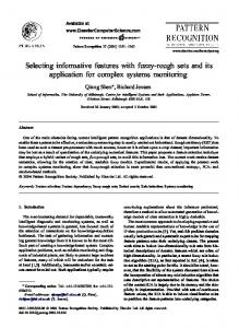
To demonstrate the improvement of our method with respect to either generative or discriminative methods, Figure 1 shows a slice view on one image by three different algorithms, and Table 2 and Table 3 give the DICE measures of all three types of structures. As we can see, The proposed algorithm significantly outperforms the two alternatives both qualitatively and quantitatively. The results of FreeSurfer [1] for the two datasets are also listed in the two tables. Our method shows competitive measures and the most stable performance among all 4 methods on the two datasets. Besides, our method takes only 20 ∼ 30 minutes to segment an MRI image, which is 5 ∼ 10 times faster than FreeSurfer under the same experimental environment. 3.3. Robustness on large datasets and more structures In this section, we show the robustness of the proposed algorithm on different MRI datasets of larger number of images with significant variations. The model in this experiment was trained from LPB40 to perform holistic segmentation (56 structures) on three datasets: (1) 492 brain images from Alzheimer’s Disease Neuroimaging Initiative (ADNI) [14] (2) A dataset from China with 160 images collected on a 1.5T scanner, and (3) A schizophrenia dataset with 226 images collected in UCLA on a 3T scanner. Figure 2 shows a number of MRI images together with the segmentation results. As we can see, the intensity patterns and textures are quite different. Even in the same dataset, ADNI, the MRI images have large variation since not all of them were acquired by the same scanner. Despite such a high degree of variation among these images, the segmentation results are mostly satisfactory in both cortical and subcortical regions. This is due to the benefit of integrating the generative model, which has the explicit parameter to account for the image appearance, and the discriminative model, which combines together a large number of informative features. We also provide DICE measures for the different datasets as quantitative evidence in Table 4. Because it is timeconsuming to annotate for the ground truth of whole brain for all images, we chose the left hippocampus as our target structure and manually annotated 68 images from ADNI, 3 images from UCLA, and 3 images from China dataset. Without changing any settings as well as the underlying model, the results of our algorithm can achieve a DICE value around 0.6 to 0.7, which is the best among the three. Although the adaptive atlas (generative model) can perform close to our algorithm on UCLA and China datasets, it is not as stable as ours when all the three datasets are taken into account. In

man brain,” Neuron, vol. 33, pp. 341–355, 2002.

(a)LPB40 1

(b)LPB40 2

(c)ADNI 1

(d)ADNI 2

[2] J. Yang, L. H. Staib, and J. S. Duncan, “Neighborconstrained segmentation with level set based 3d deformable models,” IEEE Trans. on Medical Imaging, vol. 23, no. 8, pp. 940–948, Aug. 2004. [3] Zhuowen Tu et al., “Brain anatomical structure segmentation by hybrid discriminative/generative models,” IEEE Trans. on Medical Image, vol. 27, pp. 495–508, 2008.

(e)ADNI 3

(f)ADNI 4

(g)ADNI 5

(h)ADNI 6

(i)China 1

(j)China 2

(k)UCLA 1

(l)UCLA 2

Fig. 2. Typical examples of the proposed brain segmentation method on different datasets. We use 2D slices of similar brain locations for comparison. All the results were obtained by the identical system without parameter tuning. Table 4. Average DICE value of the extracted left hippocampi by different methods. All the results were obtained by the identical system without parameter tuning. ADNI UCLA China

DM 0.541 0.551 0.495

GM 0.643 0.607 0.565

Our Algorithm 0.730 0.631 0.595

[4] J. H. Morra et al., “Automated mapping of hippocampal atrophy in 1-year repeat mri data from 490 subjects with alzheimer’s disease, mild cognitive impairment, and elderly controls,” NeuroImage, vol. 45, no. 1, pp. 3–15, 2009. [5] A. Akselrod-Ballin et al., “Atlas guided identification of brain structures by combining 3d segmentation and svm classification,” in Proc. of MICCAI, Oct. 2006. [6] K.M. Pohl et al., “A bayesian model for joint segmentation and registration,” NeuroImage, vol. 31, no. 1, pp. 228–239, 2006. [7] S. C. Zhu and A.L. Yuille, “Region competition: unifying snake/balloon, region growing and bayes/mdl/energy for multi-band image segmentation,” IEEE Trans. on PAMI, vol. 18, no. 9, pp. 884–900, Sept. 1996.

[15], the performance of FreeSurfer for hippocampus segmentation of ADNI dataset had also been addressed (0.71) and is slightly lower than our method.

[8] Z. Hou, “A review on mr image intensity inhomogeneity correction,” Int’l Jour. of Biomedical Imaging, pp. 1–11, 2006.

4. CONCLUSIONS

[9] Z. Tu, “Auto-context and its application to high-level vision tasks,” in Proc. of CVPR, Oct. 2008.

We propose a principled approach for brain MRI image segmentation by fusing together adaptive atlas (generative) and informative features through a discriminative framework. This approach uses a new way of combining generative and discriminative models. It takes advantage of the generative model being explicit and the discriminative classifier having high discrimination power. We demonstrated improved and robust results over the state-of-the-art algorithms on several clinical MRI datasets. Including a more explicit shape model may further improve our system, which is left for future research. Acknowledgments This work is funded by NSF IIS-0844566 and also supported by NIH Grant U54 RR021813 entitled Center for Computational Biology. 5. REFERENCES [1] B. Fischl et al., “Whole brain segmentation: automated labeling of neuroanatomical structures in the hu-

[10] R. P. Woods, J. C. Mazziotta, and S. R. Cherry, “Mripet registration with automated algorithm,” Journal of Computer Assisted Tomography, vol. 17, pp. 536–546, 1993. [11] D. Shattuck et al., “Construction of a 3d probabilistic atlas of human brain structures,” NeuroImage, vol. 39, no. 3, pp. 1064–1080, 2008. [12] S. M. Smith, “Fast robust automated brain extraction,” Hum Brain Mapp, vol. 17, pp. 143–155, 2002. [13] L. Ibanez et al., The ITK Software Guide Second Edition, Kitware Inc, 2005. [14] C. Jack et al., “The alzheimer’s disease neuroimaging initiative (adni): The mr imaging protocol,” Journal of MRI, 2007. [15] J. H. Morra et al., “Automatic subcortical segmentation using a contextual model,” in Proc. of 10th MICCAI, Oct. 2008.