Fuzzy Logic Programming in Action with - Scientific Research Publishing

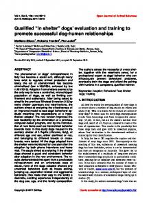
Journal of Software Engineering and Applications, 2014, 7, 273-298 Published Online April 2014 in SciRes. http://www.scirp.org/journal/jsea http://dx.doi.org/10.4236/jsea.2014.74028

Fuzzy Logic Programming in Action with  Ginés Moreno, Carlos Vázquez Department of Computing Systems, University of Castilla-La Mancha, Albacete, Spain Email: [email protected], [email protected] Received 14 February 2014; revised 10 March 2014; accepted 18 March 2014 Copyright © 2014 by authors and Scientific Research Publishing Inc. This work is licensed under the Creative Commons Attribution International License (CC BY). http://creativecommons.org/licenses/by/4.0/

Abstract During the last years, we have developed the  platform for providing a practical support to the so-called Multi-Adjoint Logic Programming approach (MALP in brief), which represents an extremely flexible framework into the Fuzzy Logic Programming arena. Nowadays,  is useful for compiling (to standard Prolog code), executing and debugging (by drawing execution trees) MALP programs, and it is ready for being extended in the near future with powerful transformation and optimization techniques designed in our research group during the recent past. Our last update consists in the integration of a graphical interface for a comfortable interaction with the system which allows, among other capabilities, the use of projects for packing scripts and auxiliary definitions of fuzzy sets/connectives, together with fuzzy programs and their associated lattices modeling truth-degrees beyond the simpler crisp case {true; false } .

Keywords Fuzzy Logic Programming, Language Design and Implementation, New Programming Concepts and Paradigms, Software Tools, Cost Measures

1. Introduction Logic programming [1] has been widely used for problem solving and knowledge representation in the past. Nevertheless, traditional pure logic programming languages (i.e., Prolog ) do not incorporate techniques or constructs to explicitly deal with uncertainty and approximated reasoning. To overcome this situation, during the last decades several fuzzy logic programming systems have been developed where the classical inference mechanism of SLD-resolution is replaced with a fuzzy variant able to handle partial truth and to reason with uncertainty, thus promoting the development of real-world applications in the fields of artificial/computational intelligence, soft-computing, semantic web, etc. Most of these systems implement the fuzzy resolution principle How to cite this paper: Moreno, G. and Vázquez, C. (2014) Fuzzy Logic Programming in Action with  . Journal of Software Engineering and Applications, 7, 273-298. http://dx.doi.org/10.4236/jsea.2014.74028

G. Moreno, C. Vázquez

introduced by Lee in [2], such as languages Prolog-Elf [3], F-Prolog [4], Fril [5], (S-)QLP [6] [7], RFuzzy [8] and MALP [9], being this last approach our target goal. Since uncertainty and vagueness are constant elements present in most human thinking activities, fuzzy logic programming seems to be a computing paradigm with a level of expressiveness very close to human reasoning. Daily, we frequently deal with fuzzy predicates (not boolean, crisp ones). For instance, a person can be quite young or not very young: the frontier between “absolutely young” and “not young at all” is not sharp, but indefinite, fuzzy. If “John” is 18 year old, we can say that he is “young” at a 95% truth degree. If “Mary” is 70 years old, she is young at a lower truth degree. Then, the obvious question is how do we model the concept of “truth degree”. In our system, we work with the so-called multi-adjoint lattices to model them by providing a flexible, wide enough definition of such notion. Informally speaking, in the multi-adjoint logic framework, a program can be seen as a set of rules each one annotated by a truth degree, and a goal is a query to the system, i.e., a set of atoms linked with connectives called aggregators. A state is a pair , σ where  is a goal and σ a substitution (initially, the identity substitution). States are evaluated in two separate computational phases. During the operational one, admissible steps (a generalization of the classical modus ponens inference rule) are systematically applied by a backward reasoning procedure in a similar way to classical resolution steps in pure logic programming, thus returning a computed substitution together with an expression where all atoms have been exploited. This last expression is then interpreted under a given lattice during what we call the interpretive phase, hence returning a pair truth_degree; substitution which is the fuzzy counterpart of the classical notion of computed answer traditionally used in LP. The main goal of this report is the detailed description of the  system which is available from http://dectau.uclm.es/floper/. Nowadays, the tool provides facilities for executing as well as for debugging (by generating declarative traces) such kind of fuzzy programs, thus fulfilling the gap we have detected in the area. In order to explain the tool, we have structured this paper as follows: in Section 2 we present the essence of MALP , including syntax, procedural semantics, and some interesting computational cost measures defined for this programming style; the core of this paper is represented by Section 3, which is dedicated to explain the main capabilities of the  system such as running/debugging MALP programs, managing lattices and dealing with additional fuzzy concepts; before finalizing in Section 5, we detail in Section 4 how the use of sophisticated multi-adjoint lattices are very useful for easily coding flexible real-world applications and obtaining low-cost traces at execution time.

2. Multi-Adjoint Logic Programming This section summarizes the main features of multi-adjoint logic programming (for a complete formulation of this framework, see [9]-[12]). In what follows, we use abbreviation MALP for referencing programs belonging to this setting.

2.1. MALP Syntax We work with a first order language,  , containing variables, constants, function symbols, predicate symbols, and several (arbitrary) connectives to increase language expressiveness: implication connectives ( ←1 , ←2 , ) ; conjunctive operators (denoted by &1 , &2 , ), disjunctive operators (|1 ,|2 ,) , and hybrid operators (usually denoted by @1 ,@ 2 , ), all of them are grouped under the name of “aggregators”. Aggregation operators (or aggregators) are useful to describe/specify user preferences. An aggregation operator, when interpreted as a truth function, may be an arithmetic mean, a weighted sum or in general any monotone application whose arguments are values of a complete bounded lattice L . For example, if an aggregator @ is interpreted as @ ( x, y, z ) = ( 3 x + 2 y + z ) 6 , we are giving the highest preference to the first argument, then to the second, being the third argument the least significant. Although these connectives are binary operators, we usually generalize them as functions with an arbitrary number of arguments. So, we often write @ ( x1 , , xn ) instead of @ ( x1 , ,@ ( xn −1 , xn ) , ) . By definition, the truth function for an n-ary aggregation operator @ : Ln → L is required to be monotonous and fulfills @ ( , ,  ) = , @( ⊥,, ⊥ ) = ⊥. Additionally, our language  contains the values of a multi-adjoint lattice equipped with a collection of adjoint pairs ←i ,&i (where each & i is a conjunctor which is intended to the evaluation of modus ponens

274

G. Moreno, C. Vázquez

[9]) formally defined as follows. Definition 2.1 (Multi-Adjoint Lattice) Let ( L, ≤ ) be a lattice. A multi-adjoint lattice is a tuple ( L, ≤, ←1 , &1 ,, ←n , &n ) such that 1) L,  is a bounded lattice, i.e. it has bottom and top elements, denoted by ⊥ and  , respectively. 2) L,  is a complete lattice, i.e. for all subset X ⊂ L , there are inf ( X ) and sup ( X ) . 3) = &i v v= &i  v , ∀v ∈ L, i =1, , n . 4) Each operation &i is increasing in both arguments. 5) Each operation ←i is increasing in the first argument and decreasing in the second one. 6) If &i , ←i is an adjoint pair in L,  then, for any x, y, z ∈ L , we have that:

x  ( y ←i z ) if and only if

( x &i z )  y

This last condition, called adjoint property, could be considered the most important feature of the framework (in contrast with many other approaches) which justifies most of its properties regarding crucial results for soundness, completeness, applicability, etc. In general, L may be the carrier of any complete bounded lattice where a L -expression is a well-formed expression composed by values and connectives defined in L , as well as variable symbols and primitive operators (i.e., arithmetic symbols such as ∗, +, min, etc...). In what follows, we assume that the truth function of any connective @ in L is given by its corresponding connective definition, that is, an equation of the form @ ( x1 ,, xn )  E , where E is a L -expression not containing variable symbols apart from x1 , , xn . For instance, consider the following classical set of adjoint pairs (conjunctions and implications) in [ 0,1] , ≤ , where labels L , G and P mean respectively Ł ukasiewicz logic, Gödel intuitionistic logic and product logic (which different capabilities for modeling pessimist, optimist and realistic scenarios, respectively): & P ( x, y )  x × y

←P ( x, y )  min (1, x y )

&G ( x, y )  min ( x, y )

1 if y ≤ x ←G ( x, y )    x otherwise ←L ( x, y )  min { x − y + 1,1}

&L ( x, y )  max ( 0, x + y − 1)

Product  Godel Łukasiewicz

Moreover, the three disjunctions associated to the previous fuzzy logics are defined as follows: |P ( x, y )  x + y − x × y , |G ( x, y )  max { x, y} , and |L ( x, y )  min { x + y,1} . At this point, we wish to make a mention to the notion of qualification domain used in the QLP ( Qualified Logic Programming) scheme described in [6], which plays a role in that framework similar to multi-adjoint lattices in MALP . A qualification domain is a structure D, , ⊥, ,  , such that D, , ⊥,  is a lattice with top (  ) and bottom ( ⊥ ) elements, a partial ordering  , and where the so-called attenuation operation “  ” is a conjunction. Now, given two elements d , e ∈ D , d  e means for the greatest lower bound of d and e , whereas d  e represents its least upper bound. We also write d  e as abbreviation of d  e & d ≠ e . The attenuation operator  satisfies the following constraints. 1)  is associative, commutative and monotonic w.r.t.  . 2) ∀d ∈ D : d  =d . 3) ∀d ∈ D : d  ⊥=⊥ . 4) ∀d , e ∈ D / {⊥, } : d  e  e . d  e1  d  e2 . 5) ∀d , e1 , e2 ∈ D : d  ( e1  e2 ) = Note that the required properties in QLP and MALP are rather close, but instead of the last distributive law just pointed out in claim 5, in our setting we use the adjoint property (claim 6 in Definition 2.1). Translations between both worlds can be frequently performed, as occurs for instance with the simple boolean qualification =  ([ 0,1] , ≤, 0,1, & ) , whose shape as a multi-adjoint lattice looks like [ 0,1] , ≤, ←, & , where & is domain de boolean conjunction and ← its adjoint implication (i.e., the usual bi-valuated logic implication). Something similar occurs with the qualification domain of Van Emden’s uncertainty values used in QLP, = ([ 0,1] , ≤, 0,1, × ) , which is equivalent to the multi-adjoint lattice (in which most of our examples are interpreted) described above,  (   ∞, ≥, ∞, 0, + ) , whose detailed explanation is delayed to as well as with the so-called weights domain = Section 4 (where we will present powerful extensions and applications related with debugging tasks into the MALP framework). In general, any qualification domain ( D, , ⊥, ,  ) whose attenuation operation  conforms an adjoint-

275

G. Moreno, C. Vázquez

pair with a given implication operation ← , can be expressed as the multi-adjoint lattice D, , ← ,  . Anyway, we wish to finish this brief comparison by highlighting that the variety of connectives definable in multi-adjoint lattices is clearly much greater than those appearing in qualification domains (where for a given program, all rules must always use the same attenuation operator), which justifies the higher expressive power of MALP w.r.t. QLP. Continuing now with the description of the multi-adjoint logic programming approach, a MALP rule is a formula H ←i  , where H is an atomic formula (usually called the head) and  (which is called the body) is a formula built from atomic formulas B1 , , Bn ( n ≥ 0 ) , truth values of L , conjunctions, disjunctions and aggregations. Rules whose body is  or equivalently, rules without body (or with empty body) are called facts. A goal is a body submitted as a query to the system. Roughly speaking, a MALP program is a set of pairs ;v (we often write “  with v ”), where  is a rule and v is a truth degree (a value of L ) expressing the confidence of a programmer in the truth of rule  . By abuse of language, we sometimes refer a tuple ;v as a “rule”. As an example, in Figure 1 we show a MALP program whose rules define fuzzy predicates modeling degrees of youth (“ y ”), heritage (“ h ”) and education (“ e ”), as well as the confidence level (“ c ”) on people for repaying a loan. Note that the seventh rule models this last notion by considering young persons having good heritage or education degrees. In what follows, we are going to explain the procedural principle of MALP programs, whose application to goal “ c ( X ) ” w.r.t. our program, will assign truth degrees 0.772 (i.e., a credibility of 77.2% ) and 0.38 (or 38% of confidence level) to “mary” and “peter”, respectively.

2.2. MALP Procedural Semantics The procedural semantics of the multi--adjoint logic language  can be thought of as an operational phase (based on admissible steps) followed by an interpretive one. In the following,  [ A] denotes a formula where A is a sub-expression which occurs in the--possibly empty--context  [ ] . Moreover,  [ A A′] means the replacement of A by A′ in context  [ ] , whereas ar ( s ) refers to the set of distinct variables occurring in the syntactic object s , and θ ar ( s )  denotes the substitution obtained from θ by restricting its domain

to ar ( s ) .

Figure 1. MALP program with admissible/interpretive derivations for goal “c(X)”.

276

G. Moreno, C. Vázquez

Definition 2.2 (Admissible Step) Let  be a goal and let σ be a substitution. The pair ; σ is a state and we denote by  the set of states. Given a program  , an admissible computation is formalized as a state AS

transition system, whose transition relation  ⊆ (  ×  ) is the smallest relation satisfying the following admissible rules (where we always consider that A is the selected atom in  and mgu ( E ) denotes the most general unifier of an equation set E [13]):

= , if θ mgu 1)  [ A] ; σ  ( [ A v &i  ]) θ ; σθ= ({ A′ A}) ,

A′ ←i ; v

= 2)  [ A] ; σ  ( [ A v ]) θ ; σθ= , if θ mgu ({ A′ A}) and

A′ ←i ; v

AS

AS

in  and  is not empty.

in  .

3)  [ A] ; σ  ( [ A ⊥ ]) ; σ , if there is no rule in  whose head unifies with A . AS

Note that the second case could be subsumed by the first one, after expressing each fact A′ ←i ; v as a program rule of the form A′ ←i ; v . Also, the third case is introduced to cope with (possible) unsuccessful AS 1

AS 2

AS 3

admissible derivations. As usual, rules are taken renamed apart. We shall use the symbols  ,  and  to distinguish between computation steps performed by applying one of the specific admissible rules. Also, the AS

application of a rule on a step will be annotated as a superscript of the  symbol. Definition 2.3 Let  be a program,  a goal and “ id ” the empty substitution. An admissible derivation AS

AS

is a sequence ; id    ′;θ . When  ′ is a formula not containing atoms (i.e., a L -expression), the pair  ′; σ , where σ = θ ar ( )  , is called an admissible computed answer (a.c.a.) for that derivation. Example 2.4 In Figure 1 we illustrate an admissible derivation (note that the selected atom in each step appears underlined), where the admissible computed answer (a.c.a.) is composed by the pair:

(

)

&P 1, &P (|P ( 0.9, 0.5 ) , 0.4 ) ;θ where θ only refers to bindings related with variables in the goal, i.e.,

= θ

X peter , X 1 peter} ar ( c ( X ) )  { X {=

peter}

If we exploit all atoms of a given goal, by applying enough admissible steps, then it becomes a formula with no atoms (a L -expression) which can be interpreted w.r.t. lattice L by applying the following definition we initially presented in [14]: Definition 2.5 (Interpretive Step) Let  be a program,  a goal and σ a substitution. Assume that @ is the truth function of connective @ in the lattice L,  associated to  , such that, for values we formalize the notion of interpretive computation r1 , , rn , rn +1 ∈ L , we have that @ ( r1 , , rn ) = rn +1 . Then, IS as a state transition system, whose transition relation  ⊆ (  ×  ) is defined as the least one satisfying: IS

 @ ( r1 , , rn )  ; σ   @ ( r1 , , rn ) rn +1  ; σ . Definition 2.6 Let  be a program and ; σ

an a.c.a., that is,  does not contain atoms (i.e., it is a IS

IS

L -expression). An interpretive derivation is a sequence ; σ   ′; σ . When  ′= r ∈ L , being L,  the lattice associated to  , the state r ; σ is called a fuzzy computed answer (f.c.a.) for that

derivation. Example 2.7 If we complete the previous derivation of Example 2.4 by applying 3 interpretive steps in order to obtain the final f.c.a. 0.38; { X peter} , we generate the interpretive derivation shown in Figure 1.

2.3. Interpretive Steps and Cost Measures A classical, simple way for estimating the computational cost required to built a derivation, consists in counting the number of computational steps performed on it. So, given a derivation D , we define its:  operational cost,  ( D ) , as the number of admissible steps performed in D .  interpretive cost,  ( D ) , as the number of interpretive steps done in D . Note that the operational and interpretive costs of derivation D1 performed in Figure 1 are  ( D1 ) = 4

277

G. Moreno, C. Vázquez

and  ( D1 ) = 3 , respectively. Intuitively,  informs us about the number of atoms exploited along a derivation. Similarly,  seems to estimate the number of connectives evaluated in a derivation. However, this last statement is not completely true:  only takes into account those connectives appearing in the bodies of program rules which are replicated on states of the derivation, but no those connectives recursively nested in the definition of other connectives. The following example highlights this fact. Example 2.8 A simplified version of rule 7 , whose body only contains an aggregator symbol is:

7* : c ( X ) ←p @1 ( h ( X ) , e ( X ) , y ( X ) ) with 1 where @1 is defined as @1 ( x1 , x2 , x3 )  &P (|P ( x1 , x2 ) , x3 ) . Note that 7* has exactly the same meaning (interpretation) than 7 , although different syntax. In fact, both ones have the same sequence of atoms in their head and bodies. The differences are regarding the set of connectives which explicitly appear in their bodies since in 7* we have moved &P and |P from the body of the rule (see 7 ) to the connective definition of @1 . Now, we use rule 7* instead of 7 for generating the following derivation D1* which returns exactly the same f.c.a than D1 : AS 17

c ( X ); id



)) ( ( & (1,@ ( 0.9, e ( peter ), y ( peter ) ) ) ; { X peter , X peter} & (1,@ ( 0.9, 0.5, y ( peter ) ) ) ; { X peter , X peter} & (1,@ ( 0.9, 0.5, 0.4 ) ) ; { X peter , X peter} &P 1,@1 h ( X 1 ), e ( X 1 ) y ( X 1 ) ; { X X 1} P

1

P

1

P

1

1

1

1

AS 2 3



AS 2 5



AS 2 1

 IS

 IS

&P (1, 0.38 ); { X peter}



0.38; { X peter} Note that, since we have exploited the same atoms with the same rules (except for the first steps performed * = = 4 . However, although with rules 7 and 7* , respectively) in both derivations, then   ( D1 )  D1 * connectives &P and |P have been evaluated in both derivations, in D1 such evaluations have not been explicitly counted as interpretive steps, and consequently they have not been added to increase the interpretive cost measure  . This unrealistic situation is reflected by the abnormal result  ( D1 ) = 3 > 2 =  D1* . It is important to note that 7* must not be considered an optimized version of 7 , even when the wrong measure  seems to indicate the contrary. This problem was initially pointed out in [15], where a preliminary solution was proposed by assigning weights to connectives in concordance with the set of primitive operators involved in the definition of the proper connective @ as well as those ones recursively contained in the definitions of connectives invoked from @ . Moreover, in [16] we improved the previous notion of “connective weight” by also taken into account the number of recursive calls to fuzzy connectives (directly or indirectly) performed in the definition of @ . A rather different way for facing the same problem is presented in [17], where instead on connective weights, we opt for the more “visual” method we have just implemented into  , based on the subsequent redefinition of the behaviour of the interpretive phase. Definition 2.9 (Small Interpretive Step) Let  be a program,  a goal and σ a substitution. Assume that the (non interpreted yet) L -expression Ω ( r1 , , rn ) occurs in  , where Ω is just a primitive operator or a connective defined in the lattice L,  associated to  , and r1 , , rn are elements of L . We formalize

( )

( )

SIS

the notion of small interpretive computation as a state transition system, whose transition relation  ⊆ (  ×  ) is the smallest relation satisfying the following small interpretive rules (where we always consider that Ω ( r1 ,, rn ) is the selected L -expression in  ):

278

G. Moreno, C. Vázquez SIS

Q Ω ( r1 , , rn )  ; σ  Q Ω ( r1 , , rn ) E ′ ; σ , if Ω is a connective defined as Ω ( x1 , , xn )  E and E ′ is obtained from the L -expression E by replacing each variable (formal parameter) xi by its corresponding value (actual parameter) ri , 1 ≤ i ≤ n , that is, E ′ = E [ x1 r1 , , xn rn ] . 1)

IS

Q Ω ( r1 , , rn )  ; σ  Q Ω ( r1 , , rn ) r  ; σ , if Ω is a primitive operator such that, once evaluated with parameters r1 , , rn , produces the result r . 2)

SIS 2

SIS 1

From now on, we shall use the symbols  and  to distinguish between computation steps performed by applying one of the specific “small interpretive” rules. Moreover, when we use the expression interpretive derivation, we refer to a sequence of small interpretive steps (according to the previous definition) instead of a sequence of interpretive steps (regarding Definition 2.5). Note that this fact supposes too a slight revision of Definition 2.6 which does not affect the essence of the notion of fuzzy computed answer: the repeated application of both kinds of small interpretive steps on a given state only affects to the length of the corresponding derivations, but both ones lead to the same final states (containing the corresponding fuzzy computed answers). Example 2.10 Recalling again the a.c.a. obtained in Example 2.4, we can reach the final fuzzy computed answer 0.38; { X peter} (achieved in Example 2.7 by means of interpretive steps) by generating now the following interpretive derivation D2 based on “small interpretive steps” (Definition 2.9):

)) ( ( (1, & (( 0.9 + 0.5) − ( 0.9 × 0.5) , 0.4)) ;{ X peter} (1, & (1.4 − ( 0.9 × 0.5), 0.4)) ;{ X peter}

& P 1, &P |P ( 0.9, 0.5 ), 0.4 ; { X peter} &P &P

P

P

& P (1, &P (1.4 − 0.45, 0.4 ) ) ; { X peter}

(

SIS 1



SIS 2



SIS 2



SIS 2



)

&P 1, &P ( 0.95, 0.4 ) ; { X peter}

SIS 1

&P (1, 0.95 × 0.4 ) ; { X peter}

SIS 2

&P (1, 0.38 ); { X peter}

SIS 1

1× 0.38; { X peter}

SIS 2









0.38; { X peter}

Going back now to Example 2.8, we can rebuild the interpretive phase of Derivation D1* in terms of small SIS 1

interpretive steps, thus generating the following interpretive derivation D2* . Firstly, by applying a  step on the L -expression & P 1,@1 ( 0.9, 0.5, 0.4 ) , it becomes &P 1, &P (|P ( 0.9, 0.5 ) , 0.4 ) , and from here, the interpretive derivation evolves exactly in the same way as derivation D2 we have just done above. At this moment, it is mandatory to meditate on cost measures regarding derivations D1 , D1* , D2 and D2* . First of all, note that the operational cost  of all them coincides, which is quite natural. However, whereas  ( D1 ) = 3 > 2 =  D1* , we have now that  ( D2 ) = 8 < 9 =  D2* . This apparent contradiction might confuse us when trying to decide which program rule ( 7 or 7* ) is “better”. The use of Definition 2.9 in derivations D2 and D2* is the key point to solve our problem, as we are going to see. In Example 2.8 we justified that by simply counting the number of interpretive steps performed in Definition 2.5 might produce abnormal results, since the evaluation of connectives with different complexities were (wrongly) measured with the same computational cost. Fortunately, the notion of small interpretive step makes visible in the proper derivation all the connectives and primitive operators appearing in the (possibly recursively nested) definitions

(

(

)

( )

)

( )

SIS 1

of any connective appearing in any derivation state. As we have seen, in D2 we have expanded in three 

279

G. Moreno, C. Vázquez SIS 2

steps the definitions of three connectives, i.e. |P , and &P twice, and we have applied five  steps to solve five primitive operators, thatSISis, + , − , and ∗ (three times). The same computational effort as been performed 1 in D2* , but also one more  step was applied to accomplish with the expansion of the extra connective @1 . This justifies why  ( D2 ) = 8 < 9 =  D2* and contradicts the wrong measures of Example 2.8: the interpretive effort developed in derivations D1 and D2 (both using the program rule 7 ), is slightly lower than the one performed in derivations D1* and D2* (which used rule 7* ), and not the contrary. The accuracy of our new way for measuring and performing interpretive computations seems to be crucial when comparing the execution behaviour of programs obtained by transformation techniques such as the fold/ unfold framework we describe in [18] [19]. In this sense, instead of measuring the absolute cost of derivations performed in a program, we are more interested in the relative gains/lost of efficiency produced on transformed programs. For instance, by applying the so-called “aggregation operation” described in [19] we can transform rule 7 into 7* and, in order to proceed with alternative transformations (fold,unfold, etc.) if the resulting program degenerates w.r.t. the original one (as occurs in this case), we need an appropriate cost measure as the one proposed here to help us for taken decisions. This fact has capital importance for discovering drastic situations which can appear in degenerated transformation sequences such as the generation of highly nested definitions of aggregators. For instance, assume the following sequence of connective definitions: @100 ( x1 , x2 )  @99 ( x1 , x2 ) , @99 ( x1 , x2 )  @98 ( x1 , x2 ) , , and finally @1 ( x1 , x2 )  x1 ∗ x2 . When trying to solve two expression of the form @99 ( 0.9, 0.8 ) and @1 ( 0.9, 0.8 ) , cost measures based on number of interpretive steps ([14]) and weights of interpretive steps ([15]) would assign 1 unit of interpretive cost to both derivations. Fortunately, our new approach is able to clearly distinguish between both cases, since the number of

( )

SIS 1

 steps performed in each one is rather different (100 and 1, respectively).

3. The “Fuzzy LOgic Programming Environment for Research”  As shown in the web page http://dectau.uclm.es/floper/ designed in our research group for freely accessing  -see also references [20]-[25]-during the last years we have been involved in the development of this tool for aliving MALP programs (which can be easily loaded into the system by means of plain-text files with extension “.fpl”). For example, our previous illustrative program included into file “P1.fpl”, contains the following rules where, note for instance that the fuzzy connectives for implication, disjunction and conjunction symbols belonging to the product logic are respectively referred as “> run. [Truth_degree = info(0.72, RULE1. RULE2.RULE3.RULE4. @AVER2.|GODEL.|LUKA. @AVER.& GODEL.&PROD.), X = a] With a very little extra effort, we can extend the previous lattice to have into account also the exploited primiSIS 2

tive operators during the interpretive phase, thus simulating  steps (see again Definition 2.9). We simply need to include a label in the Prolog definition of each primitive operator in order to identify it (for instance, “#PROD” refers to the product primitive operator). and_prod (info(X1,X2), info(Y1,Y2), info(Z1,Z2)):pri_prod (X1,Y1,Z1,DatPROD), pri_app(X2,Y2, Dat1), pri_app (Dat1, ‘&PROD.’, Dat2), pri_app(Dat2, DatPROD, Z2). pri_prod (X, Y, Z, ‘#PROD.’):- Z is X * Y. As shown in Figure 14, the result of executing again goal “p(X)” is: >> run. [Truth_degree=info(0.72, RULE1.RULE2.RULE3.RULE4. @AVER2.|GODEL.#MAX.|LUKA. #ADD.#MIN.@AVER.#ADD.#DIV. &GODEL.#MIN.&PROD.#PROD.), X = a] In this fuzzy computed answer we obtain both the truth value (0.72) and substitution ( X = a ) associated to our goal, but also the sequence of program rules exploited when applying admissible steps as well as the proper fuzzy connectives evaluated during the interpretive phase, also detailing the set of primitive operators (of the form #label) they call.

Figure 14. Obtaining declarative traces on fuzzy computed answers.

294

G. Moreno, C. Vázquez

To finish this section, we wish to mention the real-world application we have recently developed by using the  tool, where the key point is the use again of a lattice based on the Cartesian product of two previous

lattices, but whose second component, instead of strings, considers lists. In [29]-[31], we present both an interpreter and a debugger for a fuzzy variant of the XPath language, which admits new commands with a fuzzy taste for flexibly accessing XML documents, automatically generating alternative queries to retrieve more information, etc. The application can be freely downloaded and even tested on-line (see Figure 15) through http://dectau.uclm.es/fuzzyXPath/. Moreover, in [32] [33] we present our last applications recently developed with  which connect with the challenging fields of SAT/SMT and cloud computing, respectively.

5. Conclusion In the recent past, several fuzzy extensions of the popular pure logic language Prolog have been designed in order to incorporate on its core new expressive resources for dealing with uncertainty in a natural way. However, real tools for putting in practice the power of such languages are not always available to a wide audience. To reduce this gap, the experience acquired in our research group regarding the design of techniques and methods based on fuzzy logic in close relationship with the so-called multi-adjoint logic programming approach, has motivated our interest for putting in practice all our developments around the design of the  environment, which offers comfortable resources for programmers trained in declarative languages. In a first stage, we have showed that our tool is able to execute MALP programs via a “transparent compilation process” to standard Prolog code which, to the best of our knowledge, constitutes the first initiative to put in practice the integral development of this kind of fuzzy programs. Going on deeper, we have next proposed a second compilation way which produces a low-level representation of the fuzzy code, thus enabling the possibility of drawing “derivation trees” (which offer too debugging/tracing tasks) and opening the door to new program manipulation techniques such as fold/unfold-based program optimization, program specialization by partial evaluation, etc... in which we are working nowadays after being formally matured in our research group. Moreover, our tool offers the possibility of managing in a single pack, i.e. “project”, fuzzy programs with its associated multi-adjoint lattices modeled in Prolog, together with additional clauses and scripts helping to manage and increase the power of this programming tool. Our philosophy is to friendly connect this fuzzy

Figure 15. Screen-shot of an on-line work session with the XPath debugger.

295

G. Moreno, C. Vázquez

framework with Prolog programmers since our system (which can be easily installed on top of many Prolog platforms) translates the fuzzy code to classical clauses, admits the definition of sophisticated lattices for modeling advanced notions of truth degrees collecting proof traces on fuzzy computed answers and simplifies the implementation of modern, real-world applications where fuzzy logic plays an important role. As an example, our system has recently served us for developing a real-world application devoted to the flexible management of XML documents by means of a fuzzy variant of the popular XPath language. We are nowadays introducing new thresholding techniques inspired by [34] [35] for addressing in our framework the well-known “top-k ranking problem” (i.e. determining the top k answers to a query without computing the-usually wider, possibly infinite- whole set of solutions [36]-[47]).

Acknowledgements This work was supported by the EU (FEDER), and the Spanish MINECO Ministry (Ministerio de Economía y Competitividad) under grant TIN2013-45732-C4-2-P.

References [1]

Lloyd, J. (1987) Foundations of Logic Programming. 2nd Edition, Springer-Verlag, Berlin.

[2]

Lee, R. (1972) Fuzzy Logic and the Resolution Principle. Journal of the ACM, 19, 119-129. http://dx.doi.org/10.1145/321679.321688

[3]

Ishizuka, M. and Kanai, N. (1985) Prolog-ELF Incorporating Fuzzy Logic. Proceedings of the 9th International Joint Conference on Artificial Intelligence, IJCAI’85, Los Angeles, 18-23 August 1985, 701-703.

[4]

Li, D. and Liu, D. (1990) A Fuzzy Prolog Database System. John Wiley & Sons, Inc., Hoboken.

[5]

Baldwin, J.F., Martin, T.P., and Pilsworth, B.W. (1995) Fril-Fuzzy and Evidential Reasoning in Artificial Intelligence. ohn Wiley & Sons, Inc., Hoboken.

[6]

Rodrguez-Artalejo, M. and Romero-Daz, C. (2008) Quantitative Logic Programming Revisited. In: Garrigue, J. and Hermenegildo, M., Eds., Functional and Logic Programming (FLOPS’08), Springer, Berlin, 272-288.

[7]

Caballero, R., Rodrguez, M., and Romero, C.A. (2010) A Transformation-Based Implementation for CLP with Qualification and Proximity. CoRR, abs/1009.1976.

[8]

Munoz-Hernandez, S., Pablos-Ceruelo, V. and Strass, H. (2011) Rfuzzy: Syntax, Semantics and Implementation Details of a Simple and Expressive Fuzzy Tool over Prolog. Information Sciences, 181, 1951-1970. http://dx.doi.org/10.1016/j.ins.2010.07.033

[9]

Medina, J., Ojeda-Aciego, M. and Vojtáš, P. (2004) Similarity-Based Unification: A Multi-Adjoint Approach. Fuzzy Sets and Systems, 146, 43-62. http://dx.doi.org/10.1016/j.fss.2003.11.005

[10] Medina, J., Ojeda-Aciego, M. and Vojtas, P. (2001) Multi-Adjoint Logic Programming with Continuous Semantics. Proceedings of Logic Programming and Non-Monotonic Reasoning, LPNMR’01. In: Lecture Notes in Computer Science, Vol. 2173, Springer-Verlag, Berlin, 351-364. [11] Medina, J., Ojeda-Aciego, M. and Vojtas, P. (2001) A Procedural Semantics for Multi-Adjoint Logic Programing. Progress in Artificial Intelligence, EPIA’01. In: Lecture Notes in Computer Science, Vol. 2258, Springer-Verlag, Berlin, 290-297. [12] Julián, P., Moreno, G. and Penabad, J. (2009) On the Declarative Semantics of Multi-Adjoint Logic Programs. Proceedings of 10th International Work-Conference on Artificial Neural Networks, IWANN’09. In: Lecture Notes in Computer Science, Vol. 5517, Springer-Verlag, Berlin, 253-260. [13] Lassez, J.L., Maher, M.J. and Marriott, K. (1988) Unification Revisited. In: Minker, J., Ed., Foundations of Deductive Databases and Logic Programming, Morgan Kaufmann, Los Altos, 587-625. [14] Julián, P., Moreno, G. and Penabad, J. (2006) Operational/Interpretive Unfolding of Multi-Adjoint Logic Programs. Journal of Universal Computer Science, 12, 1679-1699. [15] Julián, P., Moreno, G. and Penabad, J. (2007) Measuring the Interpretive Cost in Fuzzy Logic Computations. Applications of Fuzzy Sets Theory, Proceedings of 7th International Workshop on Fuzzy Logic and Applications, WILF’07. In: Lecture Notes in Computer Science, Vol. 4578, Springer-Verlag, Berlin, 28-36. [16] Morcillo, P. and Moreno, G. (2009) On Cost Estimations for Executing Fuzzy Logic Programs. Proceedings of the 2009 International Joint Conference on Artificial Intelligence, ICAI’09, Las Vegas, 13-16 July 2009, 217-223. [17] Morcillo, P. and Moreno, G. (2009) Modeling Interpretive Steps in Fuzzy Logic Computations. Proceedings of the 8th International Workshop on Fuzzy Logic and Applications, WILF’09. In: Lecture Notes in Computer Science, Vol. 5571,

296

G. Moreno, C. Vázquez

Springer-Verlag, Berlin, 44-51.

[18] Julián, P., Moreno, G. and Penabad, J. (2005) On Fuzzy Unfolding. A Multi-Adjoint Approach. Fuzzy Sets and Systems, 154, 16-33. http://dx.doi.org/10.1016/j.fss.2005.03.013 [19] Guerrero, J. and Moreno, G. (2008) Optimizing Fuzzy Logic Programs by Unfolding, Aggregation and Folding. Electronic Notes in Theoretical Computer Science, 219, 19-34. http://dx.doi.org/10.1016/j.entcs.2008.10.032 [20] Morcillo, P. and Moreno, G. (2008) Programming with Fuzzy Logic Rules by using the FLOPER Tool. Proceedings of the 2nd Rule Representation, Interchange and Reasoning on the Web, International Symposium, RuleML’08. In: Lecture Notes in Computer Science, Vol. 3521, Springer-Verlag, Berlin, 119-126. [21] Morcillo, P., Moreno, G., Penabad, J. and Vázquez, C. (2010) Modeling Interpretive Steps into the FLOPER Environment. Proceedings of the 2010 International Conference on Artificial Intelligence, ICAI’10, Las Vegas, 12-15 July 2010, 16-22. [22] Morcillo, P., Moreno, G., Penabad, J. and Vázquez, C. (2010) A Practical Management of Fuzzy Truth Degrees Using FLOPER. Proceedings of 4th International Symposium on Rule Interchange and Applications, RuleML’10. In: Lecture Notes in Computer Science, Vol. 6403, Springer-Verlag, Berlin, 20-34. [23] Morcillo, P., Moreno, G., Penabad, J. and Vázquez, C. (2011) Declarative Traces into Fuzzy Computed Answers. Proceedings of 5th International Symposium on Rules: Research Based, Industry Focused, RuleML’11. In: Lecture Notes in Computer Science, Vol. 6826, Springer-Verlag, Berlin, 170-185. [24] Morcillo, P.J., Moreno, G., Penabad, J. and Vázquez, C. (2012) Dedekind-Macneille Completion and Cartesian Product of Multi-Adjoint Lattices. International Journal of Computer Mathematics, 89, 1742-1752. http://dx.doi.org/10.1080/00207160.2012.689826 [25] Morcillo, P., Moreno, G., Penabad, J. and Vázquez, C. (2012) String-Based Multi-Adjoint Lattices for Tracing Fuzzy Logic Computations. Electronic Communications of the EASST, 55, 17. [26] Vaucheret, C., Guadarrama, S. and Muñoz, S. (2002) Fuzzy Prolog: A Simple General Implementation Using clp(r). Proceedings of Logic for Programming, Artificial Intelligence and Reasoning, LPAR 2002. In: Lecture Notes in Computer Science, Vol. 2514, Springer-Verlag, Berlin, 450-463. [27] Rodrguez, M. and Romero, C.A. (2010) A Declarative Semantics for CLP with Qualification and Proximity. Theory and Practice of Logic Programming, 10, 627-642. http://dx.doi.org/10.1017/S1471068410000323 [28] Nguyen, H. and Walker, E. (2000) A First Course in Fuzzy Logic. Chapman & Hall/CRC, Boca Ratón. [29] Almendros-Jiménez, J., Luna, A. and Moreno, G. (2012) Fuzzy Logic Programming for Implementing a Flexible XPath-Based Query Language. Electronic Notes on Theoretical Computer Science, ENTCS, 282, 3-18. http://dx.doi.org/10.1016/j.entcs.2011.12.002 [30] Almendros-Jiménez, J., Luna, A. and Moreno, G. (2013) Annotating “Fuzzy Chance Degrees” When Debugging Xpath Queries. Advances in Computational Intelligence-Proceedings of the 12th International Work-Conference on Artificial Neural Networks, IWANN 2013 (Special Session on Fuzzy Logic and Soft Computing Application). In: Lecture Notes in Computer Science, Vol. 7903, Springer-Verlag, Berlin, 300-311. [31] Almendros-Jiménez, J., Luna, A., Moreno, G. and Vázquez, C. (2013) Analyzing Fuzzy Logic Computations with Fuzzy XPath. Actas de las XIII Jornadas sobre Programación y Lenguajes, PROLE’13, Jornadas SISTEDES, Madrid, 18-20 September 2013, 136-150. [32] Bofill, M., Moreno, G., Vázquez, C. and Villaret, M. (2013) Automatic Proving of Fuzzy Formulae with Fuzzy Logic Programming and SMT. Actas de las XIII Jornadas sobre Programación y Lenguajes, PROLE’13, Jornadas SISTEDES, Madrid, 18-20 September 2013, 151-165. [33] Vázquez, C., Tomás, L., Moreno, G. and Tordsson, J. (2013) A Fuzzy Approach to Cloud Admission Control for Safe overbooking. Proceedings of 10th International Workshop on Fuzzy Logic and Applications, WILF 2013, Genoa, 7-10 November 2013, 212-225. [34] Julián, P., Medina, J., Moreno, G. and Ojeda, M. (2010) Efficient Thresholded Tabulation for Fuzzy Query Answering. Studies in Fuzziness and Soft Computing (Foundations of Reasoning under Uncertainty), 249, 125-141. http://dx.doi.org/10.1007/978-3-642-10728-3_7 [35] Julián, P., Medina, J., Morcillo, P., Moreno, G. and Ojeda-Aciego, M. (2013) An Unfolding-Based Preprocess for Reinforcing Thresholds in Fuzzy Tabulation. In: I. Rojas, G. J. Caparrós, and J. Cabestany, Eds., IWANN (1). In: Lecture Notes in Computer Science, Vol. 7902, Springer, Berlin, 647-655. [36] Bruno, N., Chaudhuri, S. and Gravano, L. (2002) Top-K Selection Queries over Relational Databases: Mapping Strategies and Performance Evaluation. ACM Transactions on Database Systems, 27, 153-187. http://dx.doi.org/10.1145/568518.568519 [37] Chang, K.C.C. and Hwang, S.W. (2002) Minimal Probing: Supporting Expensive Predicates for Top-K Queries.

297

G. Moreno, C. Vázquez

SIGMOD Proceedings of the 2002 ACM SIGMOD International Conference on Management of DataMadison, 3-6 June 2002, 346-357.

[38] Ilyas, I.F., Aref, W.G. and Elmagarmid, A.K. (2004) Supporting Top-K Join Queries in Relational Databases. The VLDB Journal, 13, 207-221. http://dx.doi.org/10.1007/s00778-004-0128-2 [39] Chaudhuri, S., Gravano, L. and Marian, A. (2004) Optimizing Top-K Selection Queries over Multimedia Repositories. IEEE Transactions on Knowledge and Data Engineering, 16, 992-1009. http://dx.doi.org/10.1109/TKDE.2004.30 [40] Marian, A., Bruno, N. and Gravano, L. (2004) Evaluating Top-K Queries over Web-Accessible Databases. ACM Transactions on Database Systems, 29, 319-362. http://dx.doi.org/10.1145/1005566.1005569 [41] Theobald, M., Schenkel, R. and Weikum, G. (2005) Efficient and Self-Tuning Incremental Query Expansion for Top-K Query Processing. Proceedings of the 28th Annual International ACM SIGIR Conference on Research and Development in Information Retrieval, Salvador, 15-19 August 2005, 242-249. [42] Li, C., Chang, K.C.C., Ilyas, I.F. and Song, S. (2005) Ranksql: Query Algebra and Optimization for Relational Top-K Queries. SIGMOD Proceedings of the 2005 ACM SIGMOD International Conference on Management of Data, Baltimore, 13-17 June 2005, 131-142. [43] Lukasiewicz, T. and Straccia, U. (2007) Top-K Retrieval in Description Logic Programs under Vagueness for the Semantic Web. In: Prade, H. and Subrahmanian, V.S., Eds., SUM, In: Lecture Notes in Computer Science, Vol. 4772. Springer, Berlin, 16-30. [44] Re, C., Dalvi, N.N. and Suciu, D. (2007) Efficient Top-K Query Evaluation on Probabilistic Data. IEEE 23rd International Conference on Data Engineering, Istanbul, 15-20 April 2007, 886-895. [45] Eckhardt, A., Horváth, T. and Vojtás, P. (2007) Learning Different User Profile Annotated Rules for Fuzzy Preference Top-K Querying. In: Prade, H. and Subrahmanian, V.S., Eds., SUM, In: Lecture Notes in Computer Science, Vol. 4772. Springer, Berlin, 116-130. [46] Ilyas, I.F., Beskales, G. and Soliman, M.A. (2008) A Survey of Top-K Query Processing Techniques in Relational Database Systems. ACM Computing Surveys, 40, Article No. 11. [47] Prade, H. and Subrahmanian, V.S. (Eds.) (2007) Scalable Uncertainty Management. Proceedings of the 1st International Conference, SUM 2007, Washington DC, 10-12 October 2007. In: Lecture Notes in Computer Science, Vol. 4772, Springer, Berlin.

298