observer is tested in simulation and on a laboratory–scale 3D crane, while the
controller is tested ... The 3D crane is a complex electromechanical system used.
Fuzzy modeling and design for a 3D Crane P. Petrehu¸s, Zs. Lendek, P. Raica Department of Automation, Technical University of Cluj Napoca, Memorandumului 28, 400114, Cluj Napoca, Romania (e-mails: {paul.petrehus, zsofia.lendek, paula.raica}@aut.utcluj.ro). Abstract: Cranes are used to move heavy cargo. While they are in general controlled by a human operator, automated systems are able to obtain more precise control. In this paper, we design a Takagi-Sugeno (TS) fuzzy controller for the crane. For this, first a TS fuzzy model of the crane is developed, and a TS observer is used to estimate the unmeasurable states. The observer is tested in simulation and on a laboratory–scale 3D crane, while the controller is tested in simulation. Keywords: 3D Crane, discretization, fuzzy modelling, observer, controller 1. INTRODUCTION The 3D crane is a complex electromechanical system used to move heavy cargo. In general, an operator moves the crane in the desired position. The acceleration or deceleration of the crane may cause undesirable load swing. The load swing can cause human accidents, can damage the crane or the load. To control the swing, the operators need experience in crane maneuvering. Automated systems can help the operator control the load swing or can even replace the operator, (Inteco, 2008). They can also achieve precise control and increased load speed positioning (Chang and Chiang, 2009). Various control methods have been used to reduce the load swing. For example in (Chang and Chiang, 2008) the swing control is realized using a fuzzy-logic projection controller designed based on cart position and swing angle. Sawodnya et al. (2002) consider the crane as a robot and combine feedforward, feedback control, and disturbance estimation to achieve the desired position and swing control. Chang and Chiang (2009) used a PID controller for rapid positioning and a fuzzy-logic control with deadzone compensation when the crane is close to the goal for precise positioning and moving the load smoothly. Anti´c et al. (2012) designed a fuzzy-logic controller to reduce the load swing during positioning of the crane. Pauluk (2002) developed a robust control method for the crane swing and an LQ controller is used for the reference trajectory errors compensation. Pauluk et al. (2001) solve the control problem using time-optimal control. TS fuzzy models can be used to represent a large class of nonlinear systems. This type of models consist of local linear models which can represent the local input-output relations of a nonlinear system. In this paper we use a Takagi-Sugeno fuzzy representation (Takagi and Sugeno, 1985) of the crane model to design a discrete time observer and a discrete time controller that stabilizes the 3D crane. We have chosen the TS fuzzy model based approach because of its efficiency with complex nonlinear systems. To obtain the TS model we use sector nonlinearity approach (Ohtake et al., 2001). In the last decades, several methods
have been developed to analyze the stability or to design observers or controllers for TS models (Tanaka and Wang, 2001). The analysis and design conditions are usually formulated as linear matrix inequality (LMI) problems, which can be solved using available methods. This paper is organized as follows: Section II presents the nonlinear mathematical model of the crane. Section III presents the discrete time model and the equivalent TS fuzzy model. In Section IV the TS fuzzy observer is designed and simulation and experimental results for the designed observer are presented. Section V presents the TS fuzzy controller and the simulation results. Section VI provides the conclusions. 2. 3D CRANE The INTECO 3D Crane consists of a cart, moving on the xy plane, and a payload attached to a rope, which can be shifted up and down. The system is schematically presented in Fig. 1 (Inteco, 2008). For this crane a 3D mathematical model representing the movement of the system on all three axes is considered. The system has
Fig. 1. 3DCrane system: coordinates and forces
five measured quantities: xw denotes the distance of the rail of the cart from the center of the construction frame [m], yw –distance of the cart from the center of the rail [m] (xw and yw are not represented in Fig. 1), R–length of the lift-line [m], α–angle between the y axis and the lift-line [rad], β–angle between the negative direction on the z axis and the projection of the lift-line onto the xz plane [rad]. We adopt the following notations and model (Inteco, 2008): x1 = yw x6 = x˙ 5 = α˙ x2 = x˙ 1 = y˙ w x7 = β x3 = xw x8 = x˙ 7 = β˙ x4 = x˙ 3 = x˙ w
x9 = R
x5 = α x10 = x˙ 9 = R˙ Ty Tx T1 = , T2 = , T3 = mw mw + mc Fy Fx u1 = , u2 = , u3 = mw mw + mc N1 = u 1 − T 1 , N2 = u 2 − T 2 , N3 mc mc µ1 = , µ2 = mw mw + ms
Tr mc FR mc = u3 − T3
A simple nonlinear mathematical model of the crane with 3 control forces is: x˙ 1 x˙ 2 x˙ 3 x˙ 4 x˙ 5
(1)
Value
Control in y direction Control in x direction Control along the lift-line Mass of the payload [kg] Mass of the cart [kg] Mass of the moving rail [kg] Force driving the rail with cart [N ] Force driving the cart along the rail [N ] Force controlling the length of the lift-line [N ] Friction force [N ] Friction force [N ] Friction force [N ] Resultant control in x direction Resultant control in y direction Resultant control in z direction Gravitational constant [m/s2 ] Position on y axis [m] Velocity on y axis [m/s] Position on x axis [m] Velocity on x axis [m/s] Angle on x axis [rad] Angular velocity on x axis [rad/s] Angle on y axis [rad] Angular velocity on y axis [rad/s] Position on z axis [m] Velocity on z axis [m/s]
1 2.49 4.09 -
Tx Ty TR N1 N2 N3 g x1 x2 x3 x4 x5 x6 x7 x8 x9 x10 = = = = =
1 x9
100 100 75 9.81 -
x2 u∗1 + µ1 x5 u∗3 − µ1 gx5 x4 u∗2 − µ2 x7 u∗3 + µ2 gx7 x6 1 x9 + 0.1
(3)
x˙ 7 = x8 x˙ 8 = −(u∗2 − µ2 x7 u∗3 + µ2 gx7 + gx7 + 2x8 x10 )
1 x9 + 0.1
x˙ 9 = x10 x˙ 10 = u∗3
x˙ 9 = x10 x˙ 10 = −N3 + g
In Section III model (3) will be discretised and the equivalent TS fuzzy model is obtained.
where x1 , x2 , x3 , x4 , x5 , x6 , x7 , x8 , x9 , x10 are the system states. The system’s variables and parameters are presented in Table I. In order to have the equilibrium point in zero and to further simplify the mathematical model (1) we use the following change of variables:
We obtain:
Meaning
u1 u2 u3 mc mw ms Fx Fy FR
x˙ 6 = (u∗1 + µ1 x5 u∗3 − µ1 gx5 − gx5 − 2x6 x10 )
1 x˙ 6 = (N1 − µ1 x5 N3 − gx5 − 2x6 x10 ) x9 x˙ 7 = x8
x9 u∗1 u∗2 u∗3
Symbol
x˙ 1 x˙ 2 x˙ 3 x˙ 4 x˙ 5
= x2 = N1 − µ1 x5 N3 = x4 = N2 + µ2 x7 N3 = x6
x˙ 8 = −(N2 + µ2 x7 N3 + gx7 + 2x8 x10 )
Table 1. System variables and parameters
← x9 − 0.1 ← N1 ← N2 ← g − N3
3. THE DISCRETE TIME FUZZY MODEL OF THE CRANE The 3D Crane system uses discrete time to measure the variables and consequently the continuous mathematical model (3) needs to be discretised. In this section we present the discrete time TS fuzzy system for the crane. We consider the parameter values presented in Table I. 3.1 Model discretization
(2)
We consider the notation: q =
1 x9 +0.1 .
System (3) can be written as x˙ = A(x)x + B(x)u y = Cx
The system has five measured quantities, yw , xw , α, β and R which are denoted in the mathematical model by x1 , x3 , x5 , x7 , and x9 . Therefore the output matrix is: 1 0 0 00 0 00 0 0 0 0 1 0 0 0 0 0 0 0 (4) C = 0 0 0 0 1 0 0 0 0 0 0 0 0 0 0 0 1 0 0 0 0 0 0 00 0 00 1 0
To obtain the discrete time system we use the Euler discretization: Ad = Te A + I Bd = T e B (5) where A and B are the continuous system matrices, I is the identity matrix having the same dimensions as A, Te represents the sampling time and Ad and Bd are the calculated discrete time matrices. We chose the sampling time Te = 0.01 s, the same as the system data acquisition rate. Using (5) we obtain the discrete time system: x(k + 1) = Ad (x(k))x(k) + Bd (x(k))u(k) y(k) = Cx(k) (6) In the next section the equivalent TS fuzzy model of (6) is constructed using the sector non-linearity approach (Ohtake et al., 2001). 3.2 Fuzzy model for the discrete time system (6) To obtain the TS model, we use the sector non-linearity approach (Ohtake et al., 2001). With this approach, a TS model equivalent to the original nonlinear model is built. In (6), we have four nonlinear terms: x5 (k), x7 (k), q(k) = 1 x9 (k)+0.1 and x10 (k) therefore the scheduling vector z(k) = 1 , x10 (k))T . The system states are (x5 (k), x7 (k), x9 (k)+0.1 bounded, the bounds, based on the physical system are: x5 (k) ∈ [− π2 , π2 ], x10 (k) ∈ [−1, 1], x7 (k) ∈ [− π2 , π2 ] and x9 (k) ∈ [0, 0.9]. The weighting functions for zi , i = 1, ..., 4 are constructed as follows: (1) For z1 (k) = x5 (k) the bounds are z1,min = − π2 and z1,max = π2 . The weighting functions are w11 = z1,max −z1 z1,max −z1,min and w12 = 1 − w11 . The term z1 (k) can be written as z1 (k) = z1,min w11 + z1,max w12 . (2) The term z2 (k) = x7 (k) has the bounds z2,min = − π2 and z2,max = π2 . The weighting functions are w21 = z2,max −z2 z2,max −z2,min and w22 = 1 − w21 . z2 (k) can be written as z2 (k) = z2,min w21 + z2,max w22 . (3) z3 = q(k) has the following bounds z3,min = 1 and z3,max = 10. The weighting functions are w31 = z3,max −x7 z3,max −z3,min and w32 = 1 − w31 . z3 (k) = z3,min w31 + z3,max w32 . (4) For z4 (k) = x10 (k) the bounds are z4,min = −1 and z4,max = 1. The weighting functions are w41 = z4,max −z4 z4,max −z4,min and w42 = 1 − w41 . z4 (k) = z4,min w41 + z4,max w42 . As we can see above, each scheduling variable zi , i = 1, ..., 4 has 2 weighting functions, that means we have a
fuzzy model with 24 = 16 rules. The membership functions are computed as (Ohtake et al., 2001): p Y wijj (zj ) (7) hi (z) = j=1
p
with i = 1, 2, ..., 2 , ij ∈ {0, 1}, p is the number of nonlinearities, r = 2p is the number of rules. The local linear models are obtained by replacing the correspondent values of the nonlinearities in matrices Ad and Bd . For instance, one of the rules is: Model rule 1: If z1 (k) is w11 and z2 (k) is w21 and z3 (k) is w31 and z4 (k) is w41 Then x(k + 1) = Ad1 x(k) + Bd1 u(k) 1 0.01 0 0 0 0 −0.0392 0 0.6988 0 0 0 1 0.01 0 0 0 0 0.8860 0 0 0 0 0 1 Ad1 = 0 −0.3012 0 0 −0.1373 0 0 0 0 0 0 0 0.1140 0 0 0 0 0 0 0 0 0 0 0 0 0 0 0 0 0 0 0 0 0 0 0 0 0 0 0 0 0.0149 0 0 0 0.01 0 0 0 0 , 1.02 0 0 0 0 0 10.01 0 0 0 −0.1130 1.02 0 0 0 0 0 1 0.01 0 0 0 0 1 0 0 0.01 0 0 0 0 0.01 0 0 = 0.01 0 0 0 0 −0.01 0 0 0 0
Bd 1
x(k + 1) can be derived as: x(k + 1) =
16 X
0 0.0063 0 −0.0024 0 0.0063 0 0.0024 0 −0.01
hj (z(k))(Adj x(k) + Bdj u(k))
(8)
j=1
z = [zi ]T , i = 1, . . . , 4. The obtained TS system is the same as the original (6) in the considered limits. 4. THE DISCRETE TIME FUZZY OBSERVER Applying a control law requires knowing the values of states. In practice it is not possible to measure all the system states. The solution for this problem are state observers. A state observer estimates the process states relying on the process mathematical model, using the input and the output of the process.
Solving (9) for system (6), we obtain 16 observer gains. For instance, the first gain is 1 0 −0.001 0 0 0 −0.08 0 0 0.08 0 1 0 0.001 0 0 0.02 0 0.1 0 −0.02 0 1.2641 0 0 L1 = −0.12 0 26.79 0 0 0 0.002 0 1.26 0 0.15 0 26.41 0 0 0 0 0 0 1.06
0 0 0 0 0.58 This observer by design guarantees that the estimation error converges asymptotically to zero. It has to be noted that for this application one of the scheduling variables is x10 , which is not measured, and therefore its estimated value has to be used in the observer. While the design of the observer does not take this situation into account, the designed observer is stable (i.e, the estimation error converges to zero) as long as the difference between the estimated and true initial states is small enough (Bergsten, 2001). This is confirmed both by simulation and experimental results. First, we test the designed observer on simulated data. The initial conditions were x0 = [0.8381, 0.0196, 0.6813, 0.3795, ˆ 0 = 0. Fig. 2 0.8318, 0.7095, 0.4289, 0.3046, 0.1897]T and x presents the evolution of the system states for the inputs presented in Fig. 3. The evolution of error is presented in Fig. 4. To test the observer on the physical system, the initial conditions were, for x0 = 0, the Home Point of the mechanical system, while the estimated initial
x1 x2 x3 x4 x5 x6 x7 x8 x9 x10
14 12
System states
10 8 6 4 2 0 −2 0
5
10
15
Time [s]
Fig. 2. Evolution of states (simulation)
Inputs u1
i=1
ˆ (k))) + Li (y(k) − y ˆ (k) = C x ˆ (k) y where Li , i = 1, ..., r, are the observer gains. To design a stable estimator, we need to calculate positive definite matrices P , H and Mi , i = 1...r, solving the LMIs adapted from (Guerra and Vermeiren, 2004): � � −P (HAi − Mi C)T