Gait Recognition Using Motion Physics in a Neuromorphic Computing

1 Gait Recognition Using Motion Physics in a Neuromorphic Computing Framework

Ricky J. Sethi†, Amit K. Roy-Chowdhury‡, Ashok Veeraraghavan§

In this chapter, we propose a computational framework for integrating the physics of motion with the neurobiological basis of perception in order to model and recognize humans based on their gait. The neurobiological aspect of gait recognition is handled by casting our analysis within a framework inspired by Neuromorphic Computing (NMC), in which we combine the Dorsal and Ventral Pathways of the NMC model via our Integration module. We define the Hamiltonian Energy Signature (HES) to yield a representation of the motion energy required for the Dorsal Pathway and employ existing shape-based representations for the Ventral Pathway. As the core of our Integration mechanism, we utilize variants of the latest neurobiological models of feature integration and biased competition, which we implement within a statistical bootstrapping framework as Total Integration, Partial Integration, and Weighted Integration. Experimental validation of the theory is provided on the wellknown USF gait dataset, with very promising results.

1.1 Introduction Interpreting how people walk is intuitive for humans. From birth, we observe physical motion in the world around us and create perceptual models to make sense of it. Neurobiologically, we invent a framework within which we understand and interpret human activities like walking [29]. Analogously, in this chapter, we propose a computational model that seeks to understand human gait from its neural basis to its physical essence. † University of California, Los Angeles ‡ University of California, Riverside § Mitsubishi Electric Research Laboratories

1

Gait Recognition Using Motion Physics in a Neuromorphic Computing Framework 2 We thus started by examining the basis of all human activities: motion. The rigorous study of motion has been the cornerstone of physics for the last 450 years, over which physicists have unlocked a deep, underlying structure of motion. We employ ideas grounded firmly in fundamental physics that are true for the motion of the physical systems we consider in gait analysis. Using this physics-based methodology, we compute Hamiltonian Energy Signatures (HES) for a person by considering all the points on their contour, thus leading to a multi-dimensional time series that represents the gait of a person. These HES time-series curves thus provide a model of the gait for each person’s style of walking. It can also be shown using basic physical principles, that the HES is invariant under a special affine transformation, as shown in Appendix A0.1.3. This allows us to use the HES to categorize the activities of different people across different domains (high resolution, low resolution, etc.) in a moderately view-invariant manner. The HES time series, therefore, can characterize the walking styles of individuals. Note that these HES curves can be computed in either the image plane, yielding the Image HES as used in this chapter, or in the 3D world, giving the Physical HES, depending on the application domain and the nature of the tracks extracted. In either case, the Hamiltonian framework gives a highly abstract, compact representation for a system and can yield the energy of the system being considered under certain conditions. Since the perception of gait involves the interpretation of motion by the brain, we embed the above physics-based motion models within a framework inspired by Neurobiology and Neuromorphic Computing (NMC). The latest models for the perception and interpretation of motion by the brain are employed to present a novel technique for the representation and recognition of human walking styles. These models indicate that visual processing in the brain, as shown in Figure 1.1, bifurcates into two streams at V1: a Dorsal Motion Energy Pathway and a Ventral Form/Shape Pathway [47, 26]. In the Itti-Koch NMC model [40, 46], an input image is filtered in a number of low-level visual feature channels, including orientation and motion energies, as computed in the Dorsal Pathway; in our case, we use the HES to get the motion energies of a person’s gait, as outlined in Section 1.3.1. In the NMC model [46], the same low-level feature detectors as the Dorsal Pathway, acquired over very short time frames are used to classify the scene by computing a holistic, low-level signature from the Ventral Pathway; in our case, we thus use the shape features to

1.1 Introduction

3

Fig. 1.1. Neuromorphic Model for the Dorsal and Ventral Pathways: the computational modules are super-imposed onto the parts of the brain that perform similar functions, where we follow the NMC labeling convention discussed in Section 1.2.2.

classify a person’s gait as the Ventral Pathway component, as outlined in Section 1.3.2. In the NMC approach, these two pathways are combined in the Integration module, as shown in Figure 1.2. Recent research, building upon the neurobiology of object recognition, suggests the brain uses the same, or at least similar, pathways for motion recognition as it does for object recognition [18, 19, 47, 43, 26]. Although existing neurobiological models for motion recognition do posit the existence of a coupling or integration of these two pathways, they leave any specific mechanism for combination of the two pathways as an open question [18, 16]. Building upon this and recent work in the neurobiological community, which shows the dorsal and ventral processes could be integrated through a process of feature integration [49] or biased competition [10, 1, 30, 55, 9] as originally outlined by [11, 42], we propose a computational model for the Integration of the two pathways in the NMC framework by implementing this Integration in a statistical framework, creating Total Integration (only the winners from both pathways survive), Partial Integration (intermediate values are pointwise correlations of normalized measures), and Weighted Integration (Ventral values are weighted by Dorsal values and does no worse than Ventral values) models, all using the bootstrap. The bootstrap is used to find the variance of a statistic on a sample; the statistic, in our case, is the quantiles. After a

Gait Recognition Using Motion Physics in a Neuromorphic Computing Framework 4 sample is collected from an experiment, we can calculate a statistic on it (like the mean or quantiles, for example), and then use the bootstrap to figure out the variance in that statistic (e.g., via a confidence interval). The bootstrap itself works by re-sampling with replacement, as described in Section 1.3.3.

1.1.1 Overview of Chapter Building upon the fundamental principles of the physics of motion and the NMC model of perception, we present a novel framework for the modeling and recognition of humans based on their gait in video. The HES curves, developed in Section 1.3.1, give us an immediate sense of a person’s gait, as required for the motion energy aspect of the Dorsal Pathway. For the Ventral Pathway, as described in Section 1.3.2, we use shape features with DTW but we also have the freedom to use different features (e.g., image features using HMM [52], gait energy image [21], etc.). Finally, in Section 1.3.3, we incorporate the Integration module by using the neurobiological ideas of feature integration and biased competition, which we implement with a Total Integration, Partial Integration, and Weighted Integration framework using the bootstrap. This approach provides flexibility since new approaches in low-level feature extraction can be employed easily within our framework. We present detailed validation of our proposed techniques and show results on the USF gait dataset in Section 1.4.

1.2 Related Work We build liberally upon theoretical thrusts from several different disciplines, including Analytical Hamiltonian Mechanics, Neuromorphic Computing and Neurobiology, and, of course, gait analysis. The models developed for robotics in [40] provide the basic NMC architecture but are used more for object recognition and analysis. Similarly, EnergyBased Models (EBMs) [33] capture dependencies between variables for image recognition by associating a scalar “energy” to each configuration of the variables. Still others [4] take local and global optical flow approaches and compute confidence measures. Researchers have proposed computational frameworks for integration, e.g., [50], but they have also been restricted to the analysis of single images. The use of DDMCMC shown in [56] might be an excellent Integration module ap-

1.2 Related Work

5

plication for future NMC-based research thrusts and we will consider such MCMC based approaches in the future.

1.2.1 Related Work on Fusion of Multiple Features in Activity Recognition For representing the motion energy processes of the Dorsal Pathway, we propose a unique descriptor, the HES, that models the global motion of the objects involved in the activities. Our conception of the HES is based upon fundamental ideas in Classical Dynamics [32] and Quantum Mechanics [45], especially Hamilton’s Variational Principle [32]. In terms of activity recognition [24, 51], some of the cutting edge research uses the fusion of multiple features (e.g., [35]). Their approach to features fusion comes closest to the idea of combining features that express both the form and motion components. Our approach also draws inspiration from the method employed in [23], which detects global motion patterns by constructing super tracks using flow vectors for tracking high-density crowd flows in low-resolution. Our methodology, on the other hand, works in both high- and low-resolution and for densely- and sparsely-distributed objects since all it requires is the (x,y,t) tracks for the various objects. Also, our physical model goes well beyond an examination of Eulerian or Lagrangian fluid flows, which only yield local (vector) rather than global (integral) properties.

1.2.2 Related Work in Neurobiology and NMC Humans exhibit the ability to quickly understand and summarize a scene in less than 100ms. When visual information comes in from the retina, the brain seems to do some initial processing in the V1 visual cortex. Subsequently, that information bifurcates and travels along two parallel pathways in the neural model, the so-called “What” (Ventral) pathway and the “Where” (Dorsal) pathway [40]. Some NMC models [46, 40, 25] relate the ventral and dorsal processing to the ideas of gist and saliency, where the saliency component is based on low-level visual features such as luminance contrast, colour contrast, orientation, and motion energies while the gist component is a relatively lowdimensional scene representation which is acquired over very short time frames and computed as a holistic low-dimensional signature, by using the same low-level feature detectors as the saliency model. However, we use the standard notation for these two pathways (Dorsal

Gait Recognition Using Motion Physics in a Neuromorphic Computing Framework 6 and Ventral) as outlined in the latest neurobiological models of motion recognition [18, 16, 17]. Eventually, or perhaps concurrently [55], the results of these two pathways are integrated, as shown in Figure 1.1; although existing neurobiological models for motion recognition do posit the existence of a coupling or integration of these two pathways, they leave any specific mechanism for combination of the two pathways as an open question [18, 16]. Recent work in the neurobiological community shows the dorsal and ventral processes could be integrated through a process of feature integration [49] or biased competition [10, 1, 30, 55, 9].

1.2.3 Related Work in Gait recognition Recently, significant effort has been devoted to the study of human gait, driven by its potential use as a biometric for person identification. We outline some of the methods in gait-based human identification and a comprehensive review on gait recognition can be found in [38]. Role of shape and kinematics in human gait: Johansson [27] attached light displays to various body parts and showed that humans can identify motion with the pattern generated by a small set of moving dots. Muybridge [37] captured photographic recordings of humans in his study on animal locomotion. He used high speed photography images to study locomotion in humans and animals. Since then, considerable effort has been made in the Computer vision, Artificial Intelligence and Image Processing communities to the understanding of human activities from videos. A survey of work in human motion analysis can be found in [15]. Several studies have been done on the various cues that humans use for gait recognition. Hoenkamp[22] studied the various perceptual factors that contribute to the labeling of human gait. Medical studies[36] suggest that there are 24 different components to human gait. If all these different components are considered, then it is claimed that the gait signature is unique. Since it is very difficult to extract these components reliably several other representations have been used. It has been shown [7] that humans can do gait recognition even in the absence of familiarity cues. A dynamic array of point lights attached to the walker was used to record the gait pattern. It was found that static or very brief presentations are insufficient for recognition while longer displays are sufficient. Cutting and Kozlowski also suggest that dynamic cues like speed, bounciness and rhythm are more important for human recog-

1.3 Proposed Framework for Gait Analysis

7

nition than static cues like height. Cutting and Proffitt [8] argue that motion is not the simple compilation of static forms and claim that it is a dynamic invariant that determines event perception. Shape based methods: Niyogi and Adelson [39] obtained spatio-temporal solids by aligning consecutive images and use a weighted Euclidean distance to obtain recognition. Phillips et al. [41] provide a baseline algorithm for gait recognition using silhouette correlation. Han and Bhanu [21] use the gait energy image while Wang et al. use Procrustes shape analysis for recognition [54]. Foster et al. [14] use area based features. Bobick and Johnson [3] use activity specific static and stride parameters to perform recognition. Collins et al. build a silhouette based nearest neighbor classifier [5] to do recognition. Several researchers have used Hidden Markov Models (HMM) for the task of gait based identification. For example Kale et al. [28] built a continuous HMM for recognition using the width vector and the binarized silhouette as image features. A model-based method for accurate extraction of silhouettes using the HMM is provided in [34]. They use these silhouettes to perform recognition. Another shape based method for identifying individuals from noisy silhouettes is provided in [48]. Finally, [58] takes a unique shape-based approach based on gait energy image (GEI) and co-evolutionary genetic programming (CGP) for human activity classification. Kinematics based methods: Apart from these image based approaches Cunado et al. [6] model the movement of thighs as articulated pendulums and extract a gait signature using this model. But in such an approach robust estimation of thigh position in a video can be very difficult. In another kinematics based approach [2], trajectories of the various parameters of a kinematic model of the human body are used to learn a representation of a dynamical system. The parameters of the linear dynamical system are used to classify different kinds of human activities.

1.3 Proposed Framework for Gait Analysis We take an NMC-inspired approach for recognizing the walking style of people by integrating the motion signature of the objects for the Dorsal Pathway (the Hamiltonian Energy Signatures) and shape features for the Ventral Pathway via the Integration module using a variant of the neurobiological ideas of biased competition and feature integra-

Gait Recognition Using Motion Physics in a Neuromorphic Computing Framework 8

Fig. 1.2. The Neuromorphic Computing-inspired Model: the Ventral and Dorsal Pathways’ processing is combined in the Integration module using variants of feature integration and biased competition. The output of each pathway is a feature vector that is compared to the query/test using Dynamic Time Warping (DTW).

tion (please see below for detailed discussion). The overall approach is shown diagrammatically in Figure 1.2.

1.3.1 Dorsal Pathway: Hamiltonian Energy Signatures (HES) One of the most fundamental ideas in theoretical physics is the Principle of Stationary Action, also known variously as Principle of Least Action as well as Hamilton’s Variational Principle [32]. This is a variational principle that can be used to obtain the equations of motion of a system and is the very basis for most branches of physics, from Analytical Mechanics to Statistical Mechanics to Quantum Field Theory. Building upon the work of Lagrange, W.R. Hamilton applied the idea of a function whose value remains constant along any path in the configuration space of the system (unless the final and initial points are varied) to Newtonian Mechanics to derive Lagrange’s Equations, the equations of motion for the system being studied. Following Hamilton’s approach, we define Hamilton’s Action†, S, for motion along a worldline between two fixed physical events (not events in activity recognition) as: † To avoid confusion, we will use the term Action to exclusively refer to Hamilton’s Action and not action as it is normally understood in Gait Analysis.

1.3 Proposed Framework for Gait Analysis Z

9

t2

S≡

L(q(t), q(t), ˙ t)dt

(1.1)

t1

with q, the generalized coordinates †, and L, in this case, the Lagrangian which, for a conservative system, is defined as: L=T −U

(1.2)

where, T is the Kinetic Energy and U is the Potential Energy. The Hamiltonian function, derived from Hamilton’s Variational Principle (please see Appendix A0.1.1), is usually stated most compactly, in generalized coordinates, as [20]: H(q, p, t) =

X

pi q˙i − L(q, q, ˙ t)

(1.3)

i

where H is the Hamiltonian, p is the generalized momentum, and q˙ is the time derivative of the generalized coordinates, q. If the transformation between the Cartesian and generalized coordinates is timeindependent, then the Hamiltonian function also represents the total mechanical energy of the system: H(q(t), p(t)) = T (p(t)) + U (q(t))

(1.4)

In general, we compute (1.3), which depends explicitly on time, but if we have generalized coordinates and transformations from the image plane to 3D world, we can make the assumption (1.4) as a first approximation.‡ 1.3.1.1 Application to Gait Analysis This Hamiltonian is exactly what we utilize as the Hamiltonian Energy Signature (HES) of a system or sub-system observed in the given video. We end up with a quantity that provides a motion energy description of the gait: the HES (1.6), which gives a simple, intuitive expression for an † Generalized coordinates are the configurational parameters of a system; the natural, minimal, complete set of parameters by which you can completely specify the configuration of the system. In this chapter, we only deal with Cartesian coordinates, although we can deal with the more general case by using a methodology as in [12]. ‡ In this first approximation, the system can be idealized as a holonomic system, unless we deal with velocity-dependent or time-varying potentials. In fact, even when we cannot make those idealizations (e.g., viscous flows), we can define “generalized potentials” [20] and retain the standard Lagrangian, as in (1.2).

Gait Recognition Using Motion Physics in a Neuromorphic Computing Framework 10 abstract, compact representation of the system; i.e., the characteristic time-series curves for each person. We thus segment the video into systems and sub-systems (e.g., the whole body of a person, parts of the body, etc.) and, for each of those, get their tracks, from which we compute T and U, and use that to get the HES curve signature, which can then be evaluated further and the results analyzed accordingly, as shown in Figure 1.3. A system, in this sense, is defined according to the constraints of the video and the people whose walking style we are trying to identify. Thus, a system could be points on the joints of a person, points on the contour of a person, sub-sampled points on a contour, etc. More generally, the HES can be used to characterize any system or sub-system. Similarly, a human could be represented as a singular, particulate object that is part of a system of objects or as a system composed of subsystems; e.g., when we can characterize their legs, arms, hands, fingers, etc. Thus, we use the video to gain knowledge of the physics and use the physics to capture the essence of the person being observed via the HES (defined below). So now, the question is how to compute the HES from the tracks in the video. We solve this problem by using these tracks to compute the kinematic quantities that drop out of the Lagrangian formalism, thus giving a theoretical basis for examination of their energy from (x,y,t). Examples: For example, in the general case when U 6= 0, the Lagrangian, T - U, of a single person acting under a constant force, F (e.g., for a gravitational field, g, F=mg) over a distance, x, is:

L(x(t), x(t)) ˙ = 12 mv 2 − F x with x = xo + vo t + 12 at2 and a =

F m

(1.5)

We now use this Lagrangian to calculate Hamilton’s Action for the general system: Rt Rt F S = tab Ldt = tab 12 m(vo2 + 2vo m t) − F (xo + vo t) dt = 12 mvo2 (tb − ta ) − F xo (tb − ta )

(1.6)

Using Hamilton’s Variational Principle on (1.6) for a gravitational force yields (with y being the vertical position, which can be determined from the tracks):


11

1 1 mv 2 + mgh = mvo2 + mg(yb − ya ) (1.7) 2 o 2 Here, as a first approximation, we treat m as a scale factor and set it to unity; in future, we can estimate mass using the shape of the object or other heuristics, including estimating it as a Bayesian parameter. In addition, mass is not as significant when we consider the same class of objects. For more complex interactions, we can even use any standard, conservative model for U (e.g., as a spring with U = 21 kx2 for elastic interactions). In addition, we can compute more complex interactions between the points on a person’s contour. Advantages: The approach we utilize to compute H and S (which are used to calculate the HES curves) is relatively straightforward: we find tracks for the points on the contour of a silhouette, construct distance and velocity vectors from those tracks for all the relevant points on a person’s contour, and use these to compute HES vs. Time curves for each system or sub-system observed in the video. These HES curves thereby yield a compact signature for the gait of an individual and allow us to characterize different walking styles. For comparing the gaits of different people, we use the HES for each person; since the HES is already a time-series, we can compare their characteristic HES curves using a Dynamic Time Warping (DTW) algorithm. The main advantage of using the Hamiltonian formalism is that it provides a robust framework for theoretical extensions to more complex physical models. More immediately, it offers form-invariant equations, exactly as in the Lagrangian formalism, which leads to viewinvariant metrics. In addition, it can be shown that the Image HES allows us to recognize activities in a moderately view-invariant manner while the 3D Physical HES is completely view invariant; the invariance of both comes from the invariance of the HES to affine transformations, as explained in detail in the Appendix A0.1.3 with experimental validation shown in [44]. H =T +U =

1.3.2 Ventral Pathway: Shape-based Features Our construction provides flexibility since new approaches in low-level feature extraction can be employed easily within our framework. For the present work, we use shape features with DTW. In general, the Neurobiology literature suggests that orientation, shape, and color might serve as the best form-based components [29]. In particular, we used

Gait Recognition Using Motion Physics in a Neuromorphic Computing Framework 12 the approach in [53]. The integration is directly on the similarity matrices, so the exact same method can be used for other low-level features. Thus, many of the low-level approaches mentioned in Section 1.2.3 could have been used instead. Specifically, [53] presents an approach for comparing two sequences of deforming shapes using both parametric models and nonparametric methods. In their approach, Kendall’s definition of shape is used for feature extraction. Since the shape feature rests on a non-Euclidean manifold, they propose parametric models like the autoregressive model and autoregressive moving average model on the tangent space. The nonparametric model is based on Dynamic Time-Warping but they employ a modification of the Dynamic time-warping algorithm to include the nature of the non-Euclidean space in which the shape deformations take place. They apply this algorithm for gait-based human recognition on the USF dataset by exploiting the shape deformations of a person’s silhouette as a discriminating feature and then providing recognition results using the nonparametric model for gait-based person authentication.

1.3.3 NMC Integration and Gait Analysis The usual NMC tack is to integrate the Dorsal and Ventral Pathways via the Integration module, usually by weighting them, as shown in Figure 1.2. NMC and Neurobiologically-based approaches have examined different Integration methodologies, including simple pointwise multiplication, as well as exploring more standard neurobiological integration mechanisms such as feature integration [49], in which simple visual features are analyzed pre-attentively and in parallel, and biased competition [11, 42], which “proposes that visual stimuli compete to be represented by cortical activity. Competition may occur at each stage along a cortical visual information processing pathway.” There are a variety of different approaches that might be useful in simulating this Integration, including multiple hypothesis testing like Tukey HSD, MCMC techniques mentioned earlier, etc. We propose a computational approach to Integration that is a variant of these different methods and develop a computational framework that approximately mimics the neurobiological models of feature integration and biased competition [29, 10, 30]. Our final NMC implementation is outlined in Figure 1.3. We simulate the Integration via a framework in which we develop


13

Fig. 1.3. Proposed NMC-inspired Framework for Gait Analysis of USF dataset: final recognition decision is made in the Integration module. Here, a probe clip of a person walking is sent to both the Ventral and Dorsal Pathways; similarly, clips from the gallery are also sent to both pathways. Similarity measures between the probe clip and the clips in the gallery are computed from each pathway and the results integrated in the Integration module where final recognition occurs.

three different Integration variations using the bootstrap to establish the quantile analysis (explained below). In order to implement any of the Integration variants, we biased the Ventral Pathway with the Dorsal Pathway by using “feature maps” (as discussed in [55], as well as Treisman’s feature integration theory [49]), where a feature map is the distribution of features with matching peaks using a similarity measure between features. The Integration is accomplished within the overall gait recognition framework, as outlined in Algorithm 1. We start off by first creating a distance matrix for each person in a given Probe with each person in the Gallery using the method for the Ventral Pathway which, in our case, was using shape features with DTW. We also created a distance matrix for each person in that same Probe with each person in the Gallery using our method for the Dorsal Pathway, the HES characteristic curves using DTW. Finally, we apply the Integration model to the two matrices in order to get the result matrix, which contains our final matches. We implement the different Integration variants within a Hypothesis Testing framework in which, as seen above, we also use the bootstrap to ensure reasonable limits.

Gait Recognition Using Motion Physics in a Neuromorphic Computing Framework 14 Algorithm 1 Main steps of the Integration module in gait analysis Objective of the Integration Module: Given a probe clip of people walking and a gallery of people walking, match each person in the probe clip to the people in the gallery. Objective: For each Probe in list of Probes, do Integration function NMC_IT { for all (Persons in the Probe) do for all (Persons in the Gallery) do distanceMatrixVentral(i,j) = matchVentral(P ersonP robe , P ersonGallery ) distanceMatrixDorsal(i,j) = matchDorsal(P ersonP robe , P ersonGallery ) end for end for resultMatrix = INTEGRATION(distanceMatrixDorsal, distanceMatrixVentral) } The resultMatrix returned from the INTEGRATION function contains the final distance measures between each Person in the Probe vs. each Person in the Gallery. The Integration module is implemented using the bootstrap as Total Integration, Partial Integration, and Weighted Integration.

1.3.3.1 Hypothesis Testing Hypothesis testing can be considered a five-step process, given a set of distance scores of a probe sequence against all elements of the gallery: (i) Establish a null hypothesis, Ho , and an alternative hypothesis, Ha . In our case, the null hypothesis would be that a distance measure is not significant while the alternative would be that it is. (ii) Establish a significance level, α, which is usually set to 0.05 [31]. (iii) Collect the data, select the test statistic, and determine its value (observed) from the sample data (in our case, this is creating the distance matrix). (iv) Determine the criterion for acceptance/rejection of the null hypothesis by comparing the observed value to the critical value. In our case, this critical value threshold is determined via the appropriate Confidence Interval. The 2-sided Confidence Inter-


15

val will have a lower critical value of the 0.025 quantile and an upper critical value of the 0.975 quantile for α = 0.05. In our implementation, we use the bootstrap to find the variance of these quantiles (please see below for details of the bootstrap and confidence intervals). (v) Conclusion: Reject the null hypothesis if the observed value falls within the critical region (i.e., falls outside the Confidence Interval determined by the quantiles). In our case, the null hypothesis would be that all quantiles are equally significant and the alternative hypothesis would be that at least one quantile is different (i.e., is statistically significant); these significant quantiles would be the ones that fall in the critical region. 1.3.3.2 Bootstrap Following the work in [13, 57, 59], we use the bootstrap to find the variance of the desired quantile threshold used within the various BC models. Bootstrap is a nonparametric method which lets us compute some statistics when distributional assumptions and asymptotic results are not available. In statistics, it is more appealing to compute the two sided α significance threshold (confidence interval) via bootstrapping because of its accuracy and lack of assumptions. A confidence interval is a range of values that tries to quantify the uncertainty in the sample. A confidence interval can be two-sided or one-sided, as shown in Figure 1.4; e.g., the 95% 2-sided confidence interval shows the bounds within which you find 95% of the population (similarly for the 1-sided upper and lower confidence bounds). Confidence intervals are also equivalent to encapsulating the results of many hypothesis tests; if the confidence interval doesn’t include Ho , then a hypothesis test will reject Ho , and vice versa [31]; in fact, both confidence intervals and hypothesis testing are key elements of inferential statistics. This is important in our method as we utilize a hypothesis testing framework, within which we use the bootstrap to estimate the confidence intervals. The bootstrap works by re-sampling with replacement to find the variance of a statistic on a sample, as shown for our specific case in Table 1.1. We may use this algorithm twice, depending on the BC variant we’re computing: once for the upper quantile and once for the lower quantile. One way to estimate confidence intervals from bootstrap samples is to take the α and 1 − α quantiles of the estimated values, called bootstrap percentile intervals. For example, for the up-


Fig. 1.4. 2-sided and 1-sided Confidence Intervals (CI): the first diagram shows a 2-sided CI showing the confidence interval in the middle and the critical regions to the left and right; the second diagram shows a 1-sided lower bound with the critical region to the left; the final diagram shows a 1-sided upper bound with the critical region to the right; the E just indicates the mean expectation value.

per quantile, this confidence interval would then be given as CI = u u (qlower , qupper ), with lower = bN α/2c and upper = N − lower + 1, u u where N is the number of bootstrap samples and (qlower , qupper ) are the lower and upper critical values of the bootstrap confidence interval bounds. So, in our case, we use the hypothesis testing framework to establish the critical region quantiles for the Confidence Interval associated with our significance level, α, for each probe in the Distance Matrix. In order to find the variance of the desired quantiles (both lower and upper), we use the bootstrap method from Table 1.1 and Figure 1.5. We use the same significance level, α, as before and derive the bootu u ), for the upper quantile and strap critical region, CI = (qlower , qupper l l CI = (qlower , qupper ) for the lower quantile. We also use the alternate method (using just the mean of the quantile threshold) from the bootstrap for comparison. 1.3.3.3 Integration Variants It is important to note there can be different approaches to Integration as this is at the cutting edge of Neurobiological research. In this chapter, we develop three different computational models for Integration: Total Integration (using a 1-sided upper bound CI), Partial Integration (2sided CI), and Weighted Integration (2-sided CI). Total Integration (TI): In this case, only the winners survive. First, the observed distance matrix is converted into a similarity matrix; then, the bootstrap quantile analysis (shown in Table 1.1, below) is done on both the Dorsal Pathway measures and the Ventral Pathway measures

1.4 Experimental Results

17

Fig. 1.5. Overview of Bootstrap. This figure shows how the original sample is re-sampled (with replacement), say, 1000 times. In each re-sampling, a Confidence Interval is computed based on that sample. Eventually, the final Confidence Interval is estimated from either the Bootstrap Confidence Interval (on the CI computed on each re-sample) or the means (again, of the CI computed on each re-sample).

for the upper quantile only. If the value of either the Ventral or Dorsal Pathway is lower than its upper bootstrap quantile analysis confidence bound, then its value is set to 0; if both are higher than their upper bootstrap quantile analysis, the resultant value is set to the pointwise correlation between the normalized Dorsal and Ventral Pathway measures (only the values which “survive” in both are returned as the final result). Partial Integration (PI): A 2-sided CI is used in which the observed distance measure is lowered to 0 if it is less than the lower distance quantile or changed to the max value if it is greater than the upper distance quantile; intermediate values are set to the pointwise correlation between the normalized Dorsal and Ventral Pathway measures. Weighted Integration (WI): The Ventral Pathway values are weighted based on the Dorsal Pathway values; if the observed distance value of the Ventral and the Dorsal Pathway is lower than the lower distance quantile obtained from the bootstrap quantile analysis for both, then the value is set to 0; if either is higher than the upper quantile analysis, it is set to the max value; all other values are set to the unaltered Ventral Pathway value.

1.4 Experimental Results We experimented with videos from the standard USF gait dataset consisting of 67 people walking on different surfaces (grass and concrete) with different shoe types and different camera views. The Gallery contains video of four cycles of walking by all 67 people under standard conditions. There are also videos of different combinations of the 67

Gait Recognition Using Motion Physics in a Neuromorphic Computing Framework 18 Step 1: Experiment: Get DistanceMatrix DM = 2.41, 4.86, 6.06, 9.11, 10.20, 12.81, 13.17, 14.10, 15.77, 15.79 (these numbers are randomly generated numbers for illustrative purposes only as the actual distance matrices are too big to list in this example). Step 2: Re-sample: Using a pseudo-random number generator, draw a random sample of length(DM ) values, with replacement, from DM. Thus, one might obtain the bootstrap resample DM 0 = 9.11, 9.11, 6.06, 13.17, 10.20, 2.41, 4.86, 12.81, 2.41, 4.86. Note that some of the original sample values appear more than once, and others not at all Step 3: Calculate the bootstrap estimate: Compute the bootstrap percentile intervals (1 − α)100% for either the upper or the lower quantile for the resample; in this example, we might be computing the upper quantile and get q1u = 13.008 for the upper quantile of the first bootstrap run (if we were computing the lower quantile, we would get q1l for the lower quantile computed for the first bootstrap run). Step 4: Repetition: Repeat Steps 2 & 3 N (say 1000) times to obtain a total of N bootstrap u estimates: q1u , q2u , . . . , qN and sort in increasing order (if we were computing the lower l quantile, we would instead have q1l , q2l , . . . , qN ). Step 5: Parameter estimation: The desired quantile threshold is then derived from the bootstrap confidence interval, which is given as a 2-sided confidence interval: u u CI = (qlower , qupper ), where lower = bN α/2c and upper = N − lower + 1 (if we were computing the lower quantile, the bootstrap confidence interval would instead be l l , qupper ), where lower = bN α/2c and upper = N − lower + 1). Alternatively, CI = (qlower some methodologies use the mean of q1u , q2u , . . . , qnu for the desired quantile threshold of the upper quantile and the mean of q1l , q2l , . . . , qnl for the desired quantile threshold of the lower quantile.

Table 1.1. Outline of Bootstrap Quantile Analysis

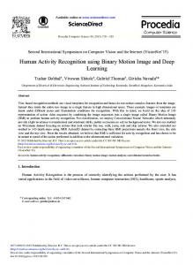
people (between 40 and 67) in the seven different probes, labelled Probe A to Probe G. The goal is then to compare the gait of each person in a probe with the gait of all the people in the Gallery to determine which one(s) it matches most closely. This is done for each of the probes in turn. Tracking and basic object-detection was already available [28] and we utilized these (x,y,t) tracks to compute the Kinetic (T) and Potential (U) energies of each point on the contour of each person (mass can be idealized to unity or computed from shape and, when we assume gait is characterized only by the horizontal motion of the body, U is set to zero). The distance and velocity vectors derived from the tracks are thereby used to compute the HES curves, which are then used as the Dorsal Pathway component of the NMC framework. The HES curve generated for each person is actually a multi-dimensional vector composed of HES curves for all the points on the contour of that person’s silhouette, as shown in Figure 1.6. We then utilized Weighted

1.4 Experimental Results

19

Fig. 1.6. Representative samples of the Multi-dimensional Vector of HES Curves for each person’s silhouette

Integration to bias the Ventral Pathway component with the Dorsal Pathway component and then used the bootstrap to set the threshold for peaks in the distributions that might compete for selection/matching. We biased these peaks by doing pointwise multiplication with the Dorsal Pathway values computed earlier to make our final selections/matches. The results are then plotted as both heatmaps of the distance matrices as well as Cumulative Match Score (CMS) graphs, which plot probability vs. rank. Figure 1.8 shows the similarity matrices and Figure 1.9 the CMS curves generated via the Weighted Integration (WI) methodology. The number of matches reported as similar, as well as the order of these matches, in each row of the Ventral Pathway method determines which method (TI, PI, or WI) does better, as reflected in the CMS curves and similarity matrices, above. For example, the CMS curves for the NMC similarity matrices for Probe A in Figure 1.8 all miss the first couple of matches (e.g., person1 to person1) since the Ventral Pathway method misses them in the first place, as seen in Figure 1.7.


Fig. 1.7. Similarity Matrices for Ventral and Dorsal Pathway approaches on Probe A

Fig. 1.8. Similarity Matrices for Total Integration, Partial Integration, and Weighted Integration on Probe A

Finally, we see the NMC approach consistently outperforms the Ventral Pathway approach alone, as seen in Table 1.2. The singular exception is Probe B in rank 1; this is because the Weighted Integration favours the Ventral Pathway method more heavily than the Dorsal Pathway method and, in this case, the Ventral Pathway method misses the real match and actually guesses matches that are far removed from the real match, as seen in the similarity matrix in Figure 1.7. In fact, analyses like this and quantile-quantile plots readily demonstrate the pres-

1.5 Conclusion

21

Fig. 1.9. CMS curves for Probes A-G using WI

ence of a shift between two distributions for most of the probes and show that the NMC always does at least as well as the Ventral Pathway method for all the probes and, in fact, usually performs better. For example, in Probe A, the Ventral Pathway method ranked 81.8% of the people correctly in rank 1 whereas the NMC approach ranked 86.4% in rank 1; in Probe D, the Ventral Pathway ranked 54.8% in rank 5 while the NMC ranked 58.1% there; in Probe F, the Ventral Pathway got 54.8% in rank 10 whereas NMC ranked 60%. Please note that although these results are specific to our Ventral Pathway approach, it is expected that similar improvements would be realized using other approaches for the pathway.

1.5 Conclusion The NMC framework and architecture provides a structured approach to gait analysis within a single, unifying framework that mimics the processing in the dorsal and ventral pathways of the human brain, as

Gait Recognition Using Motion Physics in a Neuromorphic Computing Framework 22 Table 1.2. Comparison of Ventral Pathway and NMC Integration Rank 1 and Rank 5 match probabilities for Probes A-G Probe A B C D E F G

Rank 1 Ventral 81.8 59.5 40.5 21.0 15.4 16.1 13.2

NMC 86.4 51.4 40.5 24.2 15.4 17.7 13.2

Rank 5 Ventral 92.4 81.1 70.3 54.8 46.2 41.9 34.2

NMC 92.4 83.8 70.3 58.1 46.2 43.6 34.2

understood in the neurobiology community, and is moderately viewinvariant. Our formulation takes an altogether novel approach whereby we attempt to create a theoretical framework inspired by the biological model and rooted in pure physics to gain insight into the problem of gait analysis in video. We also developed a new Dorsal Pathway feature that characterizes walking styles based on their global properties (Hamiltonian Energy Signature, HES).

1.5.1 Acknowledgments This work was partially supported by NSF grant IIS-0712253 and ARO grant W911NF-07-1-0485. We would like to acknowledge Utkarsh Gaur of the UCR Video Computing Group for many interesting discussions and feedback.

A0.1 Appendix

23

A0.1 Appendix A0.1.1 Hamilton’s Variational Principle Hamilton’s Variational Principle states that the integral, S, taken along a path of the possible motion of a physical system, is a minimum (technically, an extremum [32]) when evaluated along the actual path of motion. This variation can be expressed as: t2

Z δS = δ

(0.8)

L(q, q, ˙ t)dt = 0 t1

Here, δ is an operation that represents a variation of any system parameter by an infinitesimal amount away from the value taken by that parameter when (1.3) is an extremum. If we express L in terms of generalized coordinates,q = q(t), then the change in S when q is replaced by q+δq is arrived at by requiring that the first variation be zero [32] to yield, after integration by parts: δS =

∂L δq ∂ q˙

t2

Z

t2

+ t1

t1

∂L d ∂L − ∂q dt ∂ q˙

δqdt = 0

(0.9)

This can only be true if the integrand is zero identically, which gives rise to the so-called Euler-Lagrange equations of the Lagrangian formalism: d ∂L ∂L − =0 ∂q dt ∂ q˙

(0.10)

The Hamiltonian formalism is related to the Lagrangian formalism by the Legendre transformation, from generalized coordinates and velocities (q,q) ˙ to generalized coordinates and momenta (q,p), using the q˙ i . Thus, the Hamiltonian function is usually stated most compactly, in generalized coordinates, as [20]:

H(q, p, t) =

X

pi q˙i − L(q, q, ˙ t)

(0.11)

i

where H is the Hamiltonian, p is the generalized momentum, and q˙ is the time derivative of the generalized coordinates, q.

Gait Recognition Using Motion Physics in a Neuromorphic Computing Framework 24 A0.1.2 Deriving the Hamiltonian The procedure for deriving the Hamiltonian [20] is to first write out the Lagrangian, L, from equation (1.2) in generalized coordinates, expressing T and U in the normal manner for Lagrange’s equation. Then, the generalized momenta are calculated by differentiating the Lagrangian with respect to the generalized velocity: pi =

∂L ∂ q˙i

(0.12)

Now we can express the generalized velocities in terms of the momenta by simply inverting the result of (0.12) and using those generalized velocities in (0.11). Finally, we derive Hamilton’s Equations of Motion from the Hamiltonian equivalent of the Euler-Lagrange equations: ∂L ∂H ∂H ∂H =− = q˙i , = Fi − p˙i , ∂pi ∂qi ∂t ∂t

(0.13)

where, for a free particle with no external forces, the Fi term goes to zero, leaving: ∂H ∂L ∂H ∂H =− = q˙i , = −p˙i , ∂pi ∂qi ∂t ∂t

(0.14)

The first two relations give 2n first-order differential equations and are called Hamilton’s canonical equations of motion. This effectively results in expressing 1st-order constraints on a 2n-dimensional Phase Space, whereas the Lagrangian method expresses 2nd-order differential constraints on an n-dimensional Coordinate Space. Furthermore, if the total energy is conserved then the work, W, done on the particle had to have been entirely converted to potential energy, U. This implies that U is solely a function of the spatial coordinates (x,y,z); equivalently, U can be thought of as purely a function of the generalized configuration coordinates, qi . Rarely, U is also a function of q˙ i , making for a velocity-dependent potential, but is still independent of the time t. Noether’s theorem, in fact, guarantees that any conserved quantity (e.g., energy) corresponds to a symmetry: thus, the system can then be thought of as being independent with respect to some variable or coordinate. In this case, Noether’s theorem implies the independence of the Lagrangian with respect to time, as long as energy is conserved in this process.

A0.1 Appendix

25

A0.1.3 Invariance of HES under Affine Transformations In this section, we show the invariance of the Action which, by Equations (0.8)-(0.11), applies to H and thus, by extension, to HES, as well. We start off by using the invariance properties of the Lagrange equations; in particular, one of the properties of the Lagrange Equations is their form-invariance under coordinate transformations, especially under translations and rotations. This, in turn, implies the Action is also invariant under a Euclidean Transform (translation and rotation). We can also see this invariance from first principles by starting with the three fundamental facts of the physical world: (i) Homogeneity of Time: any instant of time is equivalent to another (ii) Homogeneity of Space: any location in space is equivalent to another (iii) Isotropy of Space: any direction in space is equivalent to another Two consequences follow from these three facts, for which there is no evidence of the contrary: (i) The mechanical properties of a closed system are unchanged by any parallel displacement of the entire system in space. (ii) The mechanical properties of a closed system do not vary when it is rotated as a whole in any manner in space. And so, three properties of the Lagrangian follow: (i) The Lagrangian of a closed system does not depend explicitly on time. (ii) The Lagrangian of a closed system remains unchanged under translations. (iii) The Lagrangian of a closed system remains unchanged under rotations. We use these basic principles in the following approach. For Lagrangian Invariance under Special Affine Transformations (translation and rotation), let the solution of the Lagrange Equations in the original coordinate system be: Z

t2

x = x(t), v = v(t) ⇒ S =

L(x(t), v(t))dt t1

(0.15)

Gait Recognition Using Motion Physics in a Neuromorphic Computing Framework 26 The solution of the Lagrange Equations for a displaced system therefore is: x ˜ = x0 + Rx(t), v˜ = Rv(t)

(0.16)

The Action calculated on the solution of the displaced system is: ⇒ S˜ =

Z

t2

Z

t2

L(˜ x, v˜)dt = t1

L(x0 + Rx(t), Rv(t))dt

(0.17)

t1

Invariance of the Lagrangian under translation gives: t2

Z ⇒

L(Rx(t), Rv(t))dt

(0.18)

t1

Invariance of the Lagrangian under rotation gives: Z

t2

⇒

L(x(t), v(t))dt = S

(0.19)

t1

Since S is the Action calculated on the solution in the original system of coordinates, this shows the invariance of the Action under rotational and translational transformations: S˜ = S

(0.20)

This also applies, by Equations (0.8)-(0.11), to H and hence shows that the HES computed from 3D points is invariant to rigid translational and rotational transformations. The HES computed from image parameters is invariant to 2D translations, rotations, and skew on the image plane as these properties are further proven for the Lagrangian in Section A0.1.3.1. We thus show that the 3D Hamiltonian is invariant to rigid 3D transformations and the Image Hamiltonian is invariant to 2D transformations. A0.1.3.1 Affine Invariance of the Lagrangian and the Action The previous section depends on the rotational and translational invariance of the Lagrangian and so, here we show that the Lagrangian is invariant under an arbitrary affine transform of World Coordinates (e.g., any combination of scaling, rotation, transform, and/or shear). This also applies to the Hamiltonian by the Legendre Transform of (0.11) since, as shown in Section A0.1.1, the Legendre Transform is used in

A0.1 Appendix

27

classical mechanics to derive the Hamiltonian formulation from the Lagrangian formulation and vice versa. Thus, we have the Lagrangian: L=T −U

(0.21)

with Kinetic Energy, T , and Potential Energy, U . The Lagrangian is a function: (0.22)

L = L (x1 , x2 , x3 , x˙ 1 , x˙ 2 , x˙ 3 ) where x1 x2 x3 are the world coordinates and x˙ i = derivatives. We first do an affine transform: yi =

X

dxi dt

are the time

Cij xj + di

(0.23)

j

Because this is an affine transform, the determinant of the matrix Cij is non-zero; i.e., |C| = 6 0. Then, the inverse matrix exists: A = C −1

(0.24)

Now we can get the formulae for xi : xi =

X

Aij yj + bi

(0.25)

j

The new Lagrangian is a complex function: L0 (y1 , y2 , y3 , y˙ 1 , y˙ 2 , y˙ 3 ) = L (x1 , x2 , x3 , x˙ 1 , x˙ 2 , x˙ 3 )

(0.26)

Where x1 , x2 , x3 , x˙ 1 , x˙ 2 , x˙ 3 are functions of y1 , y2 , y3 , y˙ 1 , y˙ 2 , y˙ 3 : x1 = x1 (y1 , y2 , y3 )

(0.27)

x2 = x2 (y1 , y2 , y3 )

(0.28)

x3 = x3 (y1 , y2 , y3 )

(0.29)

x˙ 1 = x˙ 1 (y˙ 1 , y˙ 2 , y˙ 3 )

(0.30)


x˙ 2 = x˙ 2 (y˙ 1 , y˙ 2 , y˙ 3 )

(0.31)

x˙ 3 = x˙ 3 (y˙ 1 , y˙ 2 , y˙ 3 )

(0.32)

As we can see, the Lagrangian stays invariant: L = L0 as it is just a substitution of variables and it does not change the Lagrangian value. Now we prove that Euler-Lagrange equation and Action principle are invariant under an affine transform. In Lagrangian mechanics, the basic principle is not Newton’s equation but the Action principle: the Action is a minimal, as per (0.8). The Action principle then leads to the EulerLagrange equation: ∂L d ∂L = dt ∂ x˙ i ∂xi

(0.33)

i where i = 1, 2, 3 , x1 x2 x3 are the world coordinates, and x˙ i = dx dt are the time derivatives. We now show that the Action principle, and then Euler-Lagrange equations, are invariant under an affine transform. We have an affine P transform, as in (0.23): yi = j Cij xj + di . Again, because this is an affine transform, the determinant of the matrix Cij is non-zero |C| 6= 0. Then, the inverse matrix exists, once again: A = C −1 and we can get P the formulae for xi : xi = j Aij yj + bi . The new Lagrangian is again a complex function:

L0 (y1 , y2 , y3 , y˙ 1 , y˙ 2 , y˙ 3 ) = L (x1 , x2 , x3 , x˙ 1 , x˙ 2 , x˙ 3 )

(0.34)

Where x1 , x2 , x3 , x˙ 1 , x˙ 2 , x˙ 3 are functions of y1 , y2 , y3 , y˙ 1 , y˙ 2 , y˙ 3 as in (0.27)(0.32) with time derivatives: x˙ i =

X

Aij y˙ j

(0.35)

j

Note: ∂xi = Aij ∂yj

(0.36)

∂ x˙ i = Aij ∂ y˙ j

(0.37)

A0.1 Appendix

29

We now multiply equation (0.33) by Aij and sum over i:

X ∂L X d ∂L Aij = Aij dt ∂ x˙ i ∂xi i i

(0.38)

X d ∂L ∂ x˙ i X ∂L ∂xi = dt ∂ x˙ i ∂ y˙ j ∂xi ∂yj i i

(0.39)

Using the rule of derivatives of complex functions:

X ∂L ∂xi ∂L0 = ∂xi ∂yj ∂yj i

(0.40)

X ∂L ∂ x˙ i ∂L0 = ∂ x˙ i ∂ y˙ j ∂ y˙ j i

(0.41)

∂L0 d ∂L0 = dt ∂yj ∂ y˙ j

(0.42)

Then

which is the same equation as (0.33), hence it is invariant under an affine transform and thus the Action principle is also invariant under an affine transform. Thus, Lagrangian Invariance implies Action Invariance which implies the invariance of the Euler-Lagrange equations which, in turn, implies the invariance of the HES.


Bibliography

D. M. Beck and S. Kastner, Top-down and bottom-up mechanisms in biasing competition in the human brain, Vision Research (2008). A. Bissacco, A. Chiuso, Y. Ma, and S. Soatto, Recognition of human gaits, 2 (2001), 52–57. A.F. Bobick and A. Johnson, Gait recognition using static activity-specific parameters, (2001). A. Bruhn, J. Weickert, and C. Schnorr, Lucas/kanade meets horn/schunck: combining local and global optic flow methods, IJCV, 2005, pp. 211–231. R. Collins, R. Gross, and J. Shi, Silhoutte based human identification using body shape and gait, Intl. Conf. on AFGR (2002), 351–356. D. Cunado, M.J. Nash, S.M. Nixon, and N.J Carter, Gait extraction and description by evidence gathering, Intl. Conf. on AVBPA (1994), 43–48. J.E. Cutting and L.T. Kozlowski, Recognizing friends by their walk : Gait perception without familiarity cues, Bulletin of the Psychonomic Society 9(5) (1977), 353–356. J.E. Cutting and D.R. Proffitt, Gait perception as an example of how we may perceive events, Intersensory perception and sensory integration (1981). G. Deco and T. S. Lee, The role of early visual cortex in visual integration: a neural model of recurrent interaction, European Journal of Neuroscience (2004), 1– 12. G. Deco and E. Rolls, Neurodynamics of biased competition and cooperation for attention: A model with spiking neurons, J Neurophysiol (2005), 295–313. R. Desimone and J. Duncan, Neural mechanisms of selective visual attention, Annu. Rev. Neurosci. 18 (1995), 193–222. M. Dobrski, Constructing the time independent hamiltonian from a time dependent one, Central European Journal of Physics 5 (2007), no. 3, 313–323. B. Efron and R. J. Tibshiriani, An introduction to the bootstrap, monographs on statistics and applied probability 57, Chapman & Hall, 1993. J.P. Foster, M.S. Nixon, and A. Prugel-Bennett, Automatic gait recognition using area-based metrics., Pattern Recognition Letters 24 (2003), 2489–2497. D.M. Gavrilla, The visual analysis of human movement: A survey, 73 (1999), no. 1, 82–98. M. A. Giese, Neural model for biological movement recognition, Optic Flow and Beyond, Kluwer Academic Publihers, 2004, pp. 443–470. M.A. Giese, Neural model for the recognition of biological motion, Dynamische Perzeption 2, 2000.

31

32

Bibliography

M.A. Giese and T. Poggio, Neural mechanisms for the recognition of biological movements and action, Nature Reviews Neuroscience 4 (2003), 179–192. N. H. Goddard, The perception of articulated motion: Recognizing moving light displays, Ph.D. thesis, University of Rochester, 1992. H. Goldstein, Classical mechanics, 2nd ed., Addison-Wesley, 1980. J. Han and B. Bhanu, Individual recognition using gait energy image, Workshop on MMUA (2003), 181–188. E. Hoenkamp, Perceptual cues that determine the labelling of human gait, Journal of Human Movement Studies 4 (1978), 59–69. M. Hu, S. Ali, and M. Shah, Detecting global motion patterns in complex videos, ICPR, 2008. W. Hu, T. Tan, L. Wang, and S. Maybank, A survey on visual surveillance of object motion and behaviors, IEEE Transactions on Systems, Man and Cybernetics 34 (2004), 334–352. L. Itti, C. Koch, and E. Niebur, A model of saliency-based visual attention for rapid scene analysis, PAMI, 1998, pp. 1254 – 1259. H. Jhuang, T. Serre, L. Wolf, and T. Poggio, A biologically inspired system for action recognition, ICCV, 2007. G. Johansson, Visual perception of biological motion and a model for its analysis, PandP 14 (1973), no. 2, 201–211. A. Kale, A.N Rajagopalan, Sundaresan.A., N. Cuntoor, A. Roy-Chowdhury, V. Krueger, and R. Chellappa, Identification of humans using gait, (2004). E. Kandel, J. Schwartz, and T. Jessell, Principles of neural science, 4th ed., McGraw-Hill Medical, USA, 2000. S Kastner and L Ungerleider, The neural basis of biased competition in human visual cortex, Neuropsychologia (2001), 1263–1276. G. Kochanski, Confidence intervals and hypothesis testing, 02 2005. L. Landau and E. Lifshitz, Course of theoretical physics: Mechanics, 3rd ed., 1976. Y. LeCun, S. Chopra, M. A. Ranzato, and F. Huang, Energy-based models in document recognition and computer vision, ICDAR, 2007. L. Lee, G. Dalley, and K. Tieu, Learning pedestrian models for silhoutte refinement, (2003). J. Liu, S. Ali, and M. Shah, Recognizing human actions using multiple features, CVPR, 2008. M. Murray, A. Drought, and R. Kory, Walking patterns of normal men, Journal of Bone and Joint surgery 46-A(2) (1964), 335–360. E. Muybridge, The human figure in motion, Dover Publications, 1901. M. Nixon, T. Tan, and R. Chellappa, Human identification based on gait, Springer, 2005. S.A. Niyogi and E.H. Adelson, Analyzing and recognizing walking figures in xyt, Tech. Report 223, MIT Media Lab Vision and Modeling Group, 1994. R.J. Peters and L. Itti, Beyond bottom-up: Incorporating task-dependent influences into a computational model of spatial attention, CVPR, 2007. J. Phillips, S. Sarkar, I. Robledo, P. Grother, and K.W. Bowyer, The gait identification challenge problem: Data sets and baseline algorithm, (2002). J.H. Reynolds, L. Chelazzi, and R. Desimone, Competitive mechanisms subserve attention in macaque areas v2 and v4, J. Neurosci. 19 (1999), 1736–1753. M. Riesenhuber and T. Poggio, Hierarchical models for object recognition in cortex, Nat Neuroscience 2 (1999), 1019–1025. R.J. Sethi, A.K. Roy-Chowdhury, and S. Ali, Activity recognition by integrating the physics of motion with a neuromorphic model of perception, WMVC, 2009.

Bibliography

33

R Shankar, Principles of quantum mechanics, 2nd ed., Springer, 1994. C. Siagian and L. Itti, Biologically-inspired robotics vision monte-carlo localization in the outdoor environment, IROS, 2007. R. Sigala, T. Serre, T. Poggio, and M. Giese, Learning features of intermediate complexity for the recognition of biological motion, ICANN, Springer Berlin, 2005. D. Tolliver and R.T. Collins, Gait shape estimation for identification, 4th Intl. Conf. on AVBPA (2003). A. M. Treisman and G. Gelade, A feature-integration theory of attention, Cogn. Psychol. 12 (1980), 97–136. Z. Tu, S. Zhu, and H. Shum, Image segmentation by data driven markov chain monte carlo, ICCV, 2001. P. Turaga, R. Chellappa, V. S. Subrahmanian, and O. Udrea, Machine recognition of human activities: A survey, CSVT (2008). A. Veeraraghavan, A.K. Roy-Chowdhury, and R. Chellappa, Role of shape and kinematics in human movement analysis, CVPR (2004). , Matching shape sequences in video with applications in human motion analysis, PAMI (2005). L. Wang, H. Ning, W. Hu, and T. Tan, Gait recognition based on Procrustes shape analysis, (2002). L. Yang and M. Jabri, Sparse visual models for biologically inspired sensorimotor control, Proceedings Third International Workshop on Epigenetic Robotics, 2003, pp. 131–138. A. Yuille and D. Kersten, Vision as bayesian inference: analysis by synthesis, TRENDS in Cognitive Sciences 10 (2006), no. 7, 301–308. E. Zio and F. Di Maio, Bootstrap and order statistics for quantifying thermalhydraulic code uncertainties in the estimation of safety margins, Science and Technology of Nuclear Installations (2008). X. Zou and B. Bhanu, Human activity classification based on gait energy image and coevolutionary genetic programming, ICPR 3 (2006), 556 – 559. A.M. Zoubir and B. Boashash, The bootstrap and its application in signal processing, IEEE Signal Processing Magazine 15 (1998), 56–76.