Journal of Hydrology 569 (2019) 573–586
Contents lists available at ScienceDirect
Journal of Hydrology journal homepage: www.elsevier.com/locate/jhydrol
Gap-filling of daily streamflow time series using Direct Sampling in various hydroclimatic settings
T
Moctar Dembéléa,b, , Fabio Oriania, Jacob Tumbultoc, Grégoire Mariéthoza, Bettina Schaeflia ⁎
a
University of Lausanne, Faculty of Geosciences and Environment, Institute of Earth Surface Dynamics, 1015 Lausanne, Switzerland Delft University of Technology, Faculty of Civil Engineering and Geosciences, Water Resources Section, 2628 CN Delft, Netherlands c Volta Basin Authority, Observatory for Water Resources and Related Ecosystems, 10 BP 13621 Ouagadougou 10, Burkina Faso b
ARTICLE INFO
ABSTRACT
This manuscript was handled by Andras Bardossy, Editor-in-Chief, with the assistance of Jozsef Szilagyi, Associate Editor
Complete hydrological time series are necessary for water resources management and modeling. This can be challenging in data scarce environments where data gaps are ubiquitous. In many applications, repetitive gaps can have unfortunate consequences including ineffective model calibration, unreliable timing of peak flows, and biased statistics. Here, Direct Sampling (DS) is used as a non-parametric stochastic method for infilling gaps in daily streamflow records. A thorough gap-filling framework including the selection of predictor stations and the optimization of the DS parameters is developed and applied to data collected in the Volta River basin, West Africa. Various synthetic missing data scenarios are developed to assess the performance of the method, followed by a real-case application to the existing gaps in the flow records. The contribution of this study includes the assessment of the method for different climatic zones and hydrological regimes and for different upstreamdownstream relations among the gauging stations used for gap filling. Tested in various missing data conditions, the method allows a precise and reliable simulation of the missing data by using the data patterns available in other stations as predictor variables. The developed gap-filling framework is transferable to other hydrological applications, and it is promising for environmental modeling.
Keywords: Missing values Discharge Data-driven model Stochastic method Volta River basin West Africa
1. Introduction In many regions around the world, observed streamflow records contain missing values that hinder their use for water resources management, engineering applications or hydrological modelling (Giustarini et al., 2016; Tencaliec et al., 2015). When riddled with gaps, the usability of streamflow records dwindles substantially and therefore infilling gaps in time series (Enders, 2010) is an essential step in planning, design and operation of water resources systems (Bárdossy and Pegram, 2014; Gyau-Boakye and Schultz, 1994). Missing data can occur because of the malfunctioning or failure of monitoring equipment, extreme weather conditions, limited accessibility to measurement sites, fortuitous absence of observers, humaninduced errors, budget restraints, and public turmoil or political conflicts among other factors (Berendrecht and van Geer, 2016; Elshorbagy et al., 2000; Harvey and Dixon, 2010; Mwale et al., 2012; SerratCapdevila and García Ramírez, 2016; Simonovic, 1995). Depending on the usually unpredictable factors for which missing data occurs, the gaps in the time series can vary from one time step (i.e. sub-daily to one day) to several months, or even a complete lack of data for several
⁎
years. Problems related to missing data are universal in hydrology, but exacerbated in developing countries where limited resources exist for data collection, quality assessment, repository provision, and maintenance. For many applications, the recommended approach is to infill the gaps and flag the corresponding values (Giustarini et al., 2016; GyauBoakye and Schultz, 1994; Harvey and Dixon, 2010). Thus, the user can keep track of those flagged estimates when using the data for analysis. Several methods are available for infilling gaps in hydrological records. They range from simple linear models to complex deterministic or stochastic techniques. The most common approaches include the simple nearest neighbor method by data transfer (Bárdossy and Pegram, 2014; Giustarini et al., 2016), interpolation techniques (Hughes and Smakhtin, 1996; Pappas et al., 2014; Peterson and Western, 2018; Piazza et al., 2015; Rees, 2008; Teegavarapu, 2014), autoregressive models (Bennis et al., 1997; Tencaliec et al., 2015), simple and multiple regressions (Dumedah and Coulibaly, 2011; Hirsch, 1979, 1982; Miaou, 1990; Woodhouse et al., 2006), classification and regression trees (Giustarini et al., 2016; Sidibe et al., 2018), recession methods (GyauBoakye and Schultz, 1994), recursive models (Lambert, 1969),
Corresponding author at: University of Lausanne, Faculty of Geosciences and Environment, Institute of Earth Surface Dynamics, 1015 Lausanne, Switzerland. E-mail address:
[email protected] (M. Dembélé).
https://doi.org/10.1016/j.jhydrol.2018.11.076 Received 8 August 2018; Received in revised form 7 November 2018; Accepted 30 November 2018 Available online 19 December 2018 0022-1694/ © 2018 Elsevier B.V. All rights reserved.
Journal of Hydrology 569 (2019) 573–586
M. Dembélé et al.
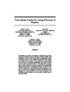
nonlinear and storage models (Coulibaly and Baldwin, 2005; Dawdy and O'Donnell, 1965), satellite data applications (Papadakis et al., 1993), dynamic state-space models (Amisigo and Van De Giesen, 2005; Berendrecht and van Geer, 2016), and various forms of artificial neural networks (Coulibaly and Evora, 2007; Dastorani et al., 2010; Elshorbagy et al., 2002; Khalil et al., 2001; Panu et al., 2000; Tfwala and Wang, 2013) among others (Bárdossy and Pegram, 2014; Dumedah and Coulibaly, 2011; Gyau-Boakye and Schultz, 1994; Harvey et al., 2012; Sidibe et al., 2018). Different studies provided a review of these methods (Gyau-Boakye and Schultz, 1994; Harvey et al., 2012; Kottegoda and Elgy, 1977; Lepot et al., 2017; Marwala, 2009; Pigott, 2001), which all have their limitations depending on the application (Amisigo and Van De Giesen, 2005; Mwale et al., 2012; Rees, 2008). For instance, the nearest neighbor method brings discontinuity in the time series (Gnauck, 2004; Lepot et al., 2017; Peterson and Western, 2018). Interpolation techniques offer a limited representation of the spacetime structure of the time series, being therefore unsuitable for periods with floods, major rainfall events, or long sequences of gaps (Di Piazza et al., 2011). Linear regression methods assume linearity between variables, which may not always be valid (Mwale et al., 2012). Multiple regression approaches ignore existing information in the target variable and need many explanatory variables, which can lead to multicolinearity issues (Miaou, 1990). Autoregression and recession models require considerable amount of data for training and validation (Amisigo and Van De Giesen, 2005). Dynamic state-space models require prior knowledge of the model parameters and the modeling system while the conditioning is done only on past observations (Amisigo and Van De Giesen, 2005; Berendrecht and van Geer, 2016). Regression trees like Random Forests (Breiman, 2001) suffer of a lack of understanding of the construction of the trees (Sidibe et al., 2018). Artificial neural networks (ANNs) have complex formulations leading to intense calculations with high computational cost (Dawson et al., 2002), and the resulting model parameters generally have no physical interpretation. A comparison of these methods is out of the scope of this research, but findings from comparison studies revealed that methods can outperform each other depending on the dataset used (Campozano et al., 2015; Harvey et al., 2012). The choice of an appropriate infilling technique depends on factors including the length of the gaps, the seasons of gap occurrence, the climatic region of the measurement sites, the length and characteristics of the existing records, the availability of ancillary or proxy data, the accuracy of the estimates versus the complexity of the approach, and the purpose of the use of the gap-filled records (Gyau-Boakye and Schultz, 1994; Mwale et al., 2012; Rees, 2008). Here, the Direct Sampling (DS) method (Mariethoz et al., 2010) is proposed as an alternative to the above approaches. It is a multiplepoint statistics (MPS) algorithm (Guardiano and Srivastava, 1993) suited to pattern reproduction. The main advantage of DS, as a stochastic method, is its ability to provide probabilistic estimates of the missing values, which allows uncertainty quantification, a very important feature in hydrograph estimation (Bárdossy and Pegram, 2014; Beven, 2016), in contrast to deterministic methods. Moreover, as a data driven approach, it can fit various data structures and simulate the outcome of a complex natural process without assuming a specific statistical model (Oriani et al., 2016). Other advantages of DS are the simplicity of its application, the multisite capability, the possibility to use auxiliary variables and predictors that contains gaps, and the ability to condition the simulation on both past and future observations for a given gap. In the present study, DS is used to infill gaps in daily streamflow data in the transboundary Volta River basin (VRB), located in West Africa. It is a data scarce region with a poor streamflow gauging density, and the available data often present long gaps in the time series (Dembélé and Mariéthoz, 2018). On average, many stations show gaps up to 80% of daily records per year, while about 10% of them have complete time series in some years between 1950 and 2016 (Fig. 1). In the VRB specifically, some studies have proposed different
Fig. 1. Proportion of missing data between 1950 and 2016 per streamflow gauging stations located in different climatic zones in the VRB.
methods to infill gaps in streamflow records. Gyau-Boakye and Schultz (1994) developed a Decision Support System for infilling missing sections of runoff time series in Ghana. Three catchments were selected to be representative of some major climatic regions in West Africa. The Decision Support System was built by comparing ten different methods based on the input data requirements in response to the availability and data characteristics of the records. Amisigo and Van De Giesen (2005) formulated a spatiotemporal linear dynamic model cast in a state-space form for patching short gaps in daily river flow data in the southern part of the VRB. They combined a Kalman filter and smoother with an expectation-maximization (EM) algorithm to estimate the state variables, the model parameters and the missing values. Taylor et al. (2006) used both a simple rainfall-runoff linear model and the Thornthwaite-Mather hydrological model (Thornthwaite and Mather, 1955) for infilling gaps in discharge data of the VRB. While these studies present valuable approaches for gap filling, they often consider a subset of the VRB, with only small data gaps. Moreover, they focus on the period from the 1930s to the 1990s, which is not necessarily representative of the most recent changes expected in the hydrological cycle of the VRB, as well as changes in water management and consumption from 2000 onwards (Mahe et al., 2010; Williams et al., 2016). Gyau-Boakye and Schultz (1994) assessed various methods, but only focusing on the southern and downstream part of the basin, and used daily data with a proportion of missing data ranging between 8% and 14% in a 15-year period. Amisigo and Van De Giesen (2005) used daily data with up to 8% of missing data per year with a deterministic approach that was applied to only one year at a time. Moreover, no station on the White Volta was considered, while it is one of the main tributaries of the Volta River, with a different hydrological regime characterized by intermittent annual flows. Taylor et al. (2006) used monthly data and reported an average of 20% but up to 50% of missing data in the records for about 20 years, with a conceptual approach that requires rainfall and evapotranspiration data, 574
Journal of Hydrology 569 (2019) 573–586
M. Dembélé et al.
which can be difficult to obtain in data scarce regions. The aim of this study is to formulate a simple infilling method that is relevant for the entire VRB and accessible to a large audience so that different water resources practitioners can adopt it. The method should be user-friendly and only require basic analytic skills, limited computational power, and solely streamflow records to avoid dependence on supplemental data. Therefore, a good candidate to that demand is the DS technique. Among other applications in geoscience, the DS algorithm has been successfully used to simulate daily rainfall data of different climatic regions in Australia (Oriani et al., 2014), self-potential data of the Volund agricultural site in Denmark (Mariethoz et al., 2015), and missing values in hydrological flows from two karst springs of the Jura mountains in Switzerland (Oriani et al., 2016). The current study extends the gap-filling approach with DS to a large number of stations and assesses for the first time the performance of the method at a large scale. The benefit of this work is the development of a thorough gap-filling framework with a stepwise implementation of the method that includes the choice of the predictor station and the setup of the algorithm. This involves the consideration of different climatic zones, the upstream-downstream and spatiotemporal relations among a large number of gauging stations with different flow regimes, the strong streamflow seasonality, and the application to an entire river basin, which altogether constitute the novelty of this study. The resulting complete daily streamflow dataset can be used for a better understanding of the water balance in the entire VRB, and more specifically for water accounting purposes (Dembélé et al., 2017b). The remainder of the paper is organized as follow. Section 2 presents the study area and the datasets used. Section 3 describes the DS method and its use for gap-filling. Section 4 presents the results of the scenario developed to test the efficiency of the DS and its application to the existing gaps in the streamflow records, with a discussion of the findings. The last section concludes and offers suggestions for future studies.
rainfall. Mean monthly temperature decreases from north to south and ranges between 27 °C and 36 °C in the north and 24 °C to 30 °C in the south (Oguntunde, 2004). The relief is quite flat as 95% of the basin lies below 400 m, and 87% of the basin is comprised between 200 and 400 m above sea level (Lemoalle and De Condappa, 2009). The distribution of seasonal rainfall and the general topography along a northsouth corridor are the two factors that determine the shape of the annual hydrograph along the principal tributaries of the Volta River (UNEP-GEF, 2013). Data acquisition in West Africa is a rather complicated task (Paturel et al., 2003; Taylor et al., 2006). For this study, daily streamflow records were obtained from different national hydrological services, regional project databases, and global online platforms (see the acknowledgement section). The time series are available between 1950 and 2016 and, for 81 streamflow gauging stations spread all over the VRB (Fig. 1), with different completeness per year and per station. In the preprocessing phase, the data collected from different sources have been quality-checked and merged into a unique dataset. As the datasets were gathered from different sources, it often happens that a gauging station has data from several sources. Therefore, a first comparison was done among the sources to complete the missing portions of the time series when they had similar data in overlapping periods. The data from the official or national data center was kept when differences were found in the data from several sources. Moreover, errors in floating point notation were corrected. No-data values were uniformed in all sources and streamflow units were converted from cfs to m3 s−1 for some stations. 3. Methodology 3.1. Direct sampling method The principle of the Direct Sampling (DS) algorithm (Mariethoz et al., 2010) is that it generates new simulated values based on a conditional resampling of a provided training dataset (TI). The newly simulated values are called simulation grid (SG). The methodology is generic and can be adapted to various application cases of stochastic conditional or unconditional simulations, requiring the definition of a specific simulation framework, i.e. the choice of the TI, the SG, the nature of the auxiliary variables, and the parametrization of the algorithm. In the proposed framework, the simulated data (stored in the SG) are sampled from the historical record of the same station (used as TI), where a similar neighborhood data pattern occurs. Only uninformed time steps (i.e. missing values in the time series) are simulated in the SG, and the existing data is used for conditioning. Other auxiliary variables can be used as conditioning dataset to better inform the simulation. The auxiliary variables can be streamflow time series from other stations. Those stations can be chosen based on their proximity and their similarity with the target station (Rees, 2008; Wagener et al., 2007). The DS implementation used in this paper is DeeSse (Straubhaar, 2017). The code is available upon request to the Randlab team at the University of Neuchâtel. Here, the target variable is simulated with one or more auxiliary variables that are used for conditioning, and can be partially or fully informed (i.e. with or without gaps). The description of the workflow for continuous variables hereafter is based on previous studies (Mariethoz et al., 2010; Oriani et al., 2014, 2016; Straubhaar et al., 2016). The inputs required for the simulation are: (1) a TI that contains the target variable Z at informed time steps, as well as auxiliary variables, and (2) a simulation grid (SG) that is a time vector hosting the simulated target variable. The time steps are uniformly spaced and identical in both TI and SG. The simulation of the target variable follows a random path and completes the SG at nonconsecutive time steps. The SG is filled progressively and becomes the actual output of the simulation. With the time vectors x = [x1, , x n] allocated to the SG and
2. Study area and dataset The Volta River basin (VRB) is one of the major drainage basin of West Africa where the number of ground-based hydro-meteorological measurements is gradually decreasing as in many other places since the 1980s (Serrat-Capdevila and García Ramírez, 2016). The VRB encompasses six countries and covers approximately 410,000 km2 (Fig. 1). The Volta River flows north to south from Burkina Faso to Ghana over a distance of 1850 km before it drains into the Atlantic Ocean at the Gulf of Guinea (Williams et al., 2016). Before reaching the Atlantic Ocean, it flows into Lake Volta, which is the World’s largest manmade lake with an area of about 8500 km2 and has been formed in 1965 as a result of the construction of the Akosombo dam in Ghana (ILEC, 2017). The river system (Fig. 1) comprises three main tributaries known as Black Volta (Mouhoun in Burkina Faso), White Volta (Nakambe in Burkina Faso) and Oti (Pendjari). The river network is poorly gauged with an estimated average density of about 3000 km2 per station (Dembélé et al., 2017a) while the World Meteorological Organization (WMO) recommends a maximum of about 1900 km2 per station (WMO, 2008). The Inter-Tropical Convergence Zone (ITCZ) controls the climate in the VRB, which varies from predominately semi-arid to sub-humid with a south-north gradient of increasing aridity. Four types of climatic zones (Fig. 1) can be identified according to the Food and Agriculture Organization (FAO) eco-climate zones classification for West Africa (FAO/GIEWS, 1998; Mul et al., 2015): (i) the Sahelian zone located in the northern part of the basin and above the 14° N parallel, with less than 500 mm yr−1 of rainfall; (ii) the Soudano-Sahelian zone located between the 11° 30′ N and 14 °N parallels, with 500–900 mm yr−1 of rainfall; (iii) the Sudanian Zone located below 11° 30′ N parallel, with 900–1100 mm yr−1 of rainfall; and (iv) the Guinean Zone extending from approximately 6° N to 10° N, with more than 1100 mm yr−1 of 575
Journal of Hydrology 569 (2019) 573–586
M. Dembélé et al.
y = [y1 , , ym ] allocated to the TI, the algorithm runs through the following steps: 1. Each continuous variable is linearly normalized to a range of [0, 1] Z ·(max (Z ) min (Z )) 1 for patterns using the transformation Z comparison at step 6. 2. A random simulation path t {1, , M } of same length as the SG is generated by doing a random permutation of the index vector in the SG. 3. An uninformed time step t of the SG is chosen for simulation by following the random simulation path. 4. A data event d (x t ) = {Z (xt + l1), , Z (x t + ln)} , representing a pattern of neighboring data of t , is retrieved from the SG according to a radius R centered on x t . It consists of at most N informed time steps, closest to x t . This defines a set of lags L = {l1, , ln} with |li | R and n N . For example, if R = 50 and N = 10 , the pattern is composed by the 10 informed time steps closest to t inside the time span [t ± 50]. The size of d (x t ) is therefore limited by N and the available informed time steps inside the search neighborhood window of 2R . 5. A random time step yi is scanned and the corresponding data event d (yi ) is retrieved to be compared with d (x t ) based on the same time lags. 6. A distance D (d (x t ), d (yi )) is calculated as a measure of dissimilarity between both data events, defined as follows:
D (d (x t ), d (yi )) =
1 n
n
| Z (x j ) j =1
Z (yj )|,
(1)
where n is the number of elements of the data event. Independently from their position, the elements of d (x t ) play an equivalent role in conditioning the simulation of Z (xt ) . The normalization at step 1 ensures the distances to be in the range [0, 1].
Fig. 2. Synthesized workflow of the DS algorithm for continuous variables. R is the radius of the search neighborhood window ([t ± R]) composed by a number of neighbors N closest to x t , with lags L = {l1, , ln} , such that li R and n N . Dmin is the minimum dissimilarity found in the TI. F is the maximum TI fraction scanned.
7. If D (d (x t ), d (yi )) is below a defined threshold T [0, 1], meaning that the two data events are sufficiently similar, the iteration stops and the datum Z (yi ) is assigned to Z (xt ) for all uninformed variables. Otherwise, the procedure is repeated from step 5 to 7 until a suitable d (yi ) is found or a prescribed TI fraction F is scanned. 8. In case no time step corresponding to D (d (x t ), d (yi )) < T is found, the datum Z (yi ) minimizing this distance is assigned to Z (xt ) . 9. The procedure from step 3 to 8 is iterated for the simulation at each x t until the entire SG is completely informed. 10. The variables are linearly back transformed to their original range.
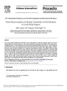
model (Oriani et al., 2014). Fig. 3 shows the simulation procedure with the DS technique. The method is implemented with the MATLAB software. The procedural implementation developed in this study will be made available to interested parties. 3.2. DS setup for gap-filling of streamflow data
The auxiliary variables simultaneously undergo the same simulation steps as Z (yt ). Fig. 2 gives a synthesized description of the DS algorithm. More details on the method can be found in the work of Mariethoz et al. (2010) and Straubhaar et al. (2016). The main DS user-defined parameters are the search window radius R , the maximum number of conditioning neighbor data N , and the threshold T for the dissimilarity measure. Each of them can have a different value for each variable. Another parameter is the maximum TI fraction scanned, called F . The resampling technique used in DS has two main features that make it different from the k-nearest neighbor bootstrap (k-NN) technique (Efron, 1992). First, the algorithm uses a random path during the simulation and completes the SG at nonconsecutive time steps. Consequently, the simulation at each x t allows conditioning on both past and future time steps, as opposed to the classical Markov chain techniques that uses a linear simulation path conditioned on past data only. Secondly, the simulation follows a variable conditioning scheme that uses the n informed neighbors closest to x t . Large-scale patterns are used at the beginning of the simulation and denser small-scale patterns toward the final iterations as the SG becomes more populated. This variable time-dependence allows the preservation of the statistical structure of the data without a prior formulation of a high-dimensional statistical
The DS setup adopted for this study is composed of the target variable Z (y ) and several auxiliary variables. A typical example of the setup is described in Table 1. Q (y ) is the streamflow at another correlated station, preferably located nearby, called the predictor station. The target variable contains the missing portions that are generated during the simulation and its informed time steps are considered as conditioning data. The correlated streamflow variable Q (y ) is given as auxiliary variable. In the example of Table 1, Q (y ) is complete, but in practice it can also present missing data. It helps restricting the uncertainty and provides guidance around the missing values. Considering the strong annual seasonality of streamflow in the VRB, two out-ofphase periodic triangular functions (A1 (y ) and A2 (y )) , each with a period of 365.25 days, are used as auxiliary variables to constrain the position of the simulated values inside the annual cycle. Another auxiliary variable is the recession indicator H (y ) , computed based on Q (y ) and used to constrain the occurrence of high and low flows. It takes a value of H = 0 for a rising hydrograph limb and H = 1 during a recession. Its computation requires two user-defined parameters (w, v ) as follows: the minimum and maximum (local extremes) of Q (y ) are identified inside a moving temporal window [y ± w]. Each new extreme is considered only when its difference with the previous 576
Journal of Hydrology 569 (2019) 573–586
M. Dembélé et al.
Fig. 3. Sequential simulation of streamflow time series with DS. The dashed rectangle represents the search window defined as twice the radius R , and contains the data event that is formed by the simulated datum in green and the N neighboring data in red. (For interpretation of the references to colour in this figure legend, the reader is referred to the web version of this article.)
extreme is greater than v , and the next extreme is of a different type (minimum or maximum). A logical test is finally used to obtain H . A rising limb is activated with a local minimum until the occurrence of a local maximum activates a recessing limb, with a continuous alternation of both states (Oriani et al., 2016). The values w [10 30] and v [80 120] are used in the current setup. The DS parameters for each variable for an example of TI are given in Table 1. Following Meerschman et al. (2013), the DS parameters values were taken in the ranges: R [100 300], N [3 20] and T [0.002 0.1]. R and N are in the unit of the time series in the TI, and T is unitless. For variables A1 (y ) and A2 (y ) which have a predictable behavior, high-order conditioning is not necessary and therefore R and N are set to 1. The maximum TI fraction scanned is set to F = 0.5 for all the simulations.
This value allows sampling a sufficient portion of the TI and avoids the phenomenon of verbatim copy, which results in mimicking portions of the TI (Meerschman et al., 2013). 3.3. Calibration and evaluation In a first step, a calibration procedure is carried out to obtain an adequate set of DS parameters. Contrary to the DS setup in (Oriani et al., 2016), where the target variable Z (y ) and the predictor variable Q (y ) have the same DS parameters, in this case study all variables can have different parameters values. Consequently, several sets of parameters are used to simulate the same time series and the resulting realizations are compared to the reference data using six pairwise
Table 1 Example of a training dataset (TI) with DS parameters (R : search window radius; N : maximum number of conditioning neighbor data; T : distance threshold; and F : maximum TI fraction scanned, F = 0.5).
577
Journal of Hydrology 569 (2019) 573–586
M. Dembélé et al.
statistical indicators. The statistical indicators, as described in Dembélé and Zwart (2016), are: (1) the Pearson correlation coefficient (r ) that evaluates the strength and the direction of the linear association of two variables; (2) the Spearman rank-order correlation coefficient (rs ) that estimates the degree of the monotonic relationship; (3) the Mean Error (ME ) that assesses the average estimate error; (4) the Bias that reflects the degree to which the reference value is systematically over- or underestimated; (5) the root mean square error (RMSE ) that measures the average magnitude of the estimate errors; (6) and the Nash–Sutcliffe Efficiency coefficient (NSE ) that shows how well the estimate predicted the observed time series. The best set of parameters is chosen as the one yielding the smallest prediction error. The rank of each set of parameters is calculated for each of the statistical indicators. The best set of parameters is taken as the one with the best cumulative rank. As observed in previous applications (Meerschman et al., 2013; Oriani et al., 2016), the algorithm is suitable for such a manual setup since it has a low number of algorithmic parameters which are relatively well defined for a given application. All results are evaluated based on visual comparison and statistical indicators. Quantile-Quantile (QQ) plots (Chambers, 2017) are used to compare the probability distribution of the simulated gap portions and reference data portions, for daily QQplots. The monthly and yearly QQ-plots represent the 1-month and 1year moving average of daily values for the entire reconstructed time series.
station Q (y ) that is fully informed (i.e. without gaps). Those scenarios are numbered with odd numbers between 1 and 9. The predictor stations in scenarios 1 and 3, the Yarugu and Nuwuni stations respectively, belong to the same sub-catchment as the target station Daboya. However, in scenarios 5, 7 and 9, the predictor stations, Akosombo, Lawra and Saboba respectively, belong to different sub-catchments from Daboya. They are located downstream of the Lower Volta, Black Volta and Oti sub-catchments (Fig. 1), respectively. Therefore, they all receive streamflow from different sub-catchments and with different characteristics from that of Daboya. The five remaining scenarios, numbered with even numbers between 2 and 10, are duplicates of the scenarios in the first group with the exception that the time series of the predictor stations are not fully informed (i.e. contain gaps). For each scenario, Z (y ) always contains 50% of gaps, and when Q (y ) contains gaps, they represent 30% of the time series or about 2 out of 6 years of missing values. To determine whether the dependence between target and predictor variables is maintained in the simulated values, the corresponding correlations before and after simulation are given in Table 3 for each scenario. The predictor variables are chosen purposely to have some with weak correlation and others with strong correlation with the target variable. For each scenario, ten realizations of the target variable are produced. A comparison of DS with the linear regression method is carried out and the results can be found in the Supplementary materials (SM Fig.1). After demonstrating the performance of the DS for infilling gaps in streamflow time series with various scenarios, the method is used to infill real gaps in the streamflow records of the VRB. The predictor station selection and the simulation procedure are described hereafter.
3.4. Gap-filling framework This section presents the approach adopted for gap-filling of streamflow data in a large river basin with different gauging stations and climatic zones, using the VRB as a case study. First, the DS performance is assessed on a set of scenarios with artificial gaps created in the target variable. Secondly, the method is used to infill real gaps in streamflow records. The following sections give a description of the experimental set-up for each of the above-mentioned steps.
3.4.2. Predictor station selection for real gaps reconstruction The selection of the most appropriate predictor station is not a trivial task (Giustarini et al., 2016; Harvey et al., 2012; Peterson and Western, 2018). Here, the most similar station to the target station is chosen as predictor. Only one predictor is used to condition the target station (Harvey et al., 2012; Hughes and Smakhtin, 1996): this avoids conflicting information among potential predictors, prevents unrealistic simulated time-series structures, and reduces computational time. Therefore, the choice of the predictor station is crucial and depends on its similarity with the target station (Rees, 2008; Wagener et al., 2007). Both r and rs are used to estimate the statistical similarity of the variables. When several stations show the same correlation with the target station, the one with the longest overlapping time steps, the smallest proportion of gaps and the highest spatial proximity (Rees, 2008) with the target is chosen as the predictor station. A similar approach for the predictor station selection is adopted in the work of Giustarini et al. (2016). A priority index based on these criteria allows ranking all the stations of the river network from the one that is easiest to be gap-filled, to the one that is the most challenging. In a first run, only the overlapping periods are simulated, i.e. common years of data between the target and the predictor stations. Thereafter, the next best predictor candidate is considered to simulate the remaining portions. This procedure is executed with different predictors until a fully informed SG is
3.4.1. Experimental set-up for various gap scenarios To assess the DS performance, artificial random gaps are created inside the streamflow records of some stations having long and complete records. Representative stations are selected based on their locations in different sub-catchments with specific climatic and physical characteristics to account for different hydroclimatic settings in the VRB (Fig. 1). For each station, a predictor station Q (y ) is selected, which can be fully or partially informed. The Daboya station is chosen as the target station for all the gap-filling scenarios proposed hereafter. It is located at the outlet of the White Volta sub-catchment and receives the water drained from the semi-arid to the sub-humid zone of the VRB. A strong annual seasonality of the streamflow is depicted in Fig. 4, which also shows the artificial gaps. The randomly created gaps vary in size from 5 to 30 consecutive days and represent 50% of the whole time series over a period of 6 years. Ten scenarios (Table 3) are developed to assess the performance of the DS method. Among them, five scenarios are developed by simulating Z (y ) with the time series of a predictor
Fig. 4. Time series of the target station with artificial gaps.
578
Journal of Hydrology 569 (2019) 573–586
M. Dembélé et al.
Table 2 Applications for real gaps reconstruction (App: application, WV: White Volta, BV: Black Volta, LV: Lower Volta, Q position: predictor station position relative to the target). App
Target (Z)
Predictor (Q)
Q position
Z length (years)
missing in Z (%)
catchment
r (Z, Q)
rs (Z, Q)
1 2 3 4 5 6
Daboya Saboba Dapola Lawra Kpong Akosombo
Nawuni Mango Lawra Dapola Akossombo Kpong
upstream upstream upstream downstream upstream downstream
26 39 60 60 31 31
18 21 15 22 4 0.05
WV Oti BV
0.85 0.95 0.93
0.86 0.94 0.93
LV
0.89
0.89
Table 3 Pearson (r (Z , Q) ) and the Spearman (rs (Z , Q) ) correlation coefficients between the target (Z ) and the predictor (Q ) variables (SC: same catchment; indicates where the target and the predictor stations are located. SN: scenario number, CN: catchment name, WV: White Volta, BV: Black Volta, LV: Lower Volta). Before gaps, Z and Q are fully informed. After gaps, Z (Daboya station) contains 50% of gaps for all scenarios, while Q contains 30% of gaps for only even-numbered scenarios.
Fig. 5. Boxplots of six statistical indicators (Y-axis) of the realizations for the ten gap-filling scenarios (X-axis). The statistical indicators (r , rs , NSE , Bias , ME , and RMSE ) are computed only between the simulated missing portions of the newly simulated target variable (Zsim ) and their corresponding values in the reference target variable (Z ) .
obtained. In case there is no other predictor that overlaps the remaining non-covered portions of the data after the first run, the first predictor is used to fully inform the SG.
3.4.3. Simulation procedure for real gaps The simulation is done in two steps: (1) additional gaps are created in the target variable before the simulation. A calibration is done based on the simulation of these newly created gaps only. It allows obtaining a suitable set of parameters that yield the best scores for the statistical 579
Journal of Hydrology 569 (2019) 573–586
M. Dembélé et al.
indicators in Section 3.3. This step is similar to the scenarios (Section 3.4.1), but additional gaps are created in the target variable that already contains gaps; (2) the suitable set of parameters obtained in the first step is used to simulate the real missing values in the target variable, and therefore to reconstruct the entire time series. Six applications (Table 2) for real gaps reconstruction are presented and discussed using representative stations of the hydrological regimes, the agro-climatic zones, and the sub-catchments of the VRB. The fourth and the sixth applications are duplicates of the third and the fifth respectively, with the exception that the predictor station becomes the target and vice versa. This inversion is done to assess the influence of the upstream-downstream position of the predictor station on the performance of the simulation. Five hundred realizations are produced per application.
and the corresponding reference values (Fig. 5). The parameters used for the simulation are given in Table 4 for each scenario. 4.2. Time series reconstruction for different scenarios Fig. 6 shows the time series of the reconstructed target variable and the corresponding predictor station. The average scores of the statistical indicators are given alongside the plots. Flow duration curves for the scenarios are provided in Supplementary material (SM Fig. 2). Except for scenario 1, only scenarios where the predictor variable contains artificial gaps are presented because they represent the most challenging cases and are the most likely situation in data scarce regions. A comparison between scenarios 1 and 2 highlights an increase in the width of the simulation ensemble, meaning a higher uncertainty in the prediction, and a deviation of the mean of the realizations from the reference time series (Z (y ) ), when the predictor variable (Q (y ) ) is not fully informed (scenario 2). A visual check of the scenarios shows that the realizations ensemble usually contains the target variable. Mismatches often depend on the predictor station used. In scenario 2, the target and predictor stations are located in the same sub-catchment but they are weakly correlated (r (Z , Q ) = 0.69). The realizations mostly cover the reference time series but miss some local flow peaks, predict some false high flows, and show lags in the prediction. This is due to the inability to sample a similar data pattern in the predictor variable, therefore suboptimal patterns are chosen. In scenario 4, the reconstructions are of high quality because the target and predictor stations are in the same sub-catchment and strongly associated (r (Z , Q ) = 0.99). The overall prediction is excellent in scenario 4. The average magnitude of the simulation error (RMSE = 61.44 m3 s−1) is due to the unmet peak flows but this is balanced by the alternation of under- and overestimated high flows, which finally results in a smallME = −2.3 m3 s−1. In scenarios 6, 8 and 10, the target and the predictor stations are located in different catchments. In scenario 6, a negative and low correlation is observed between the variables (r (Z , Q ) = −0.43). The predictor station measures the discharge of the Akosombo dam located downstream of the Lower Volta sub-catchment (Fig. 1). This scenario is the most challenging and is not recommended even if the results show acceptable prediction performance (NSE = 0.76). The RMSE is higher as observed during the second year of the simulation period. The under- and overestimated flow portions balance and result in a small average error withME = −2.36 m3 s−1. However, this might not be the case for a shorter or longer period of simulation. Consequently, simulating the target variable with a poorly informative predictor station is not advisable. In scenario 8 (r (Z , Q ) = 0.91), the predictor station is located in the Black Volta sub-catchment, where the main river is perennial and characterized by low flows. Conversely, the river gauged by the target station is mainly not perennial in its upstream part and is characterized
4. Results and discussion 4.1. Gap-filling scenarios evaluation In Table 3, the minimum and maximum values of the Pearson (r (Z , Q ) ) and the Spearman (rs (Z , Q ) ) correlation coefficients among the ten realizations highlight the possibility of obtaining a similar target variable with the same strength and degree of association with the predictor variable as before the simulation and before creating the artificial gaps. The correlation values r (Z , Q ) and rs (Z , Q ) before the simulation usually lie in the same range as after the simulation, with an average error of 2%. Therefore, DS is able to preserve the correlation between the target and the predictor stations. However, this statistical relation is preserved more or less faithfully depending on the performance in reproducing the missing portions. The capability of the DS to reproduce the missing portions of the target variable is highlighted in Fig. 5. DS usually performs better when the predictor station is fully informed. For that reason and due to the recurrence of gaps in the collected data in the VRB, attention is paid to the even-numbered scenarios from 2 to 10 (Table 3), which represent the scenarios with gaps in the predictor variable. In this regard, scenario 4 outperforms the other scenarios for all statistical indicators. It is followed by scenarios 10, 2, and 8 in increasing order. Scenario 6 gives the weakest scores. This performance in scenario 6 can be linked to the negative and weak correlation between the target and predictor station (Table 3). Notwithstanding that scenario 6 gives the lowest performance, it still has good scores in terms of prediction. Such results might have been possible due to the parameters optimization step preceding the simulation. Therefore, a relevant set of parameters is obtained for a good prediction. The overall performance of the DS is good and for all scenarios considered according to the statistical indicators calculated only between the simulated portions
Table 4 DS parameters for the gap-filling scenarios. (see Section 3.2 for parameters and variables description). Scenarios
DS parameters for all variables in TI R
1 3 5 7 9 2 4 6 8 10
N
T
A 1, A 2
H
Q
Z
A1, A2
H
Q
Z
A 1, A 2
H
Q
Z
1 1 1 1 1 1 1 1 1 1
200 200 200 200 200 200 200 200 200 200
200 200 200 200 200 200 200 200 200 200
200 200 200 200 200 200 200 200 200 200
1 1 1 1 1 1 1 1 1 1
10 10 10 10 10 10 10 10 10 10
7 7 3 7 7 3 3 7 3 7
3 3 7 3 3 3 3 3 7 3
0.05 0.05 0.05 0.05 0.05 0.05 0.05 0.05 0.05 0.05
0.1 0.1 0.1 0.1 0.1 0.1 0.1 0.1 0.1 0.1
0.02 0.002 0.02 0.02 0.01 0.07 0.002 0.07 0.05 0.05
0.02 0.005 0.005 0.002 0.005 0.005 0.002 0.02 0.02 0.02
580
Journal of Hydrology 569 (2019) 573–586
M. Dembélé et al.
Fig. 6. Selected gap-filling scenarios. The six statistical indicators compare the reference to the simulated values only, and represent the average for ten realizations produced per scenario. Q (y ) is shifted on the y-axis (y-shift) for display purpose.
by a long low flow period followed by a short high flow period with a long recession time. The mean of the realizations matches well the reference time series, except for some extreme flows as in the third, fourth and fifth years. Despite a narrow ensemble range, the evaluation scores are lower than those of scenario 4. In scenario 10 (r (Z , Q ) = 0.95), the predictor station is located downstream of the Oti sub-catchment where the river drains the steepest region of the VRB, and is characterized by a long low flow period followed by a short high flow period with a short recession time. The prediction shows good average evaluation scores, with some mismatches of local flow peaks and time lags in the second,
third, and fifth years. The scores in scenario 10 are slightly better than those in scenario 8. This can be due to the higher proximity of the predictor station to the target station in scenario 10, which presents similar hydrological regimes and climate conditions. The alternating under- and overestimation of flow extremes, when they occur, are balanced over time and result in a low average error. This brings to attention a possible improvement or conservation of the statistical content of the predicted time series at a lower temporal resolution. This assumption is investigated in the next section. In addition, DS performs generally well compared to the linear regression 581
Journal of Hydrology 569 (2019) 573–586
M. Dembélé et al.
Fig. 7. Comparison of the empirical probability distribution of the reconstructed artificial gaps (Y-axis) against the corresponding reference data (X-axis) for each scenario, using daily (a, b), monthly (c, d), and yearly (e, f) QQ-plots. The dots represent the median of the realizations and the dashed lines indicate the 5th and 95th percentiles. The predictor variable is partially informed in even-numbered scenarios (b–d–f) and fully informed in odd-numbered scenarios (a–c–e). All units are in m3 s−1. Table 5 DS parameters for the reconstruction of real gaps. (see Section 3.2 for parameters and variables description). App
Target (Z)
Predictor (Q)
DS parameters for all variables in TI R
1 2 3 4 5 6
Daboya Saboba Dapola Lawra Kpong Akosombo
Nawuni Mango Lawra Dapola Akosombo Kpong
N
T
A1, A2
H
Q
Z
A1, A2
H
Q
Z
A1, A2
H
Q
Z
1 1 1 1 1 1
200 200 200 200 200 200
200 200 200 200 200 200
200 200 200 200 200 200
1 1 1 1 1 1
10 10 10 10 10 10
5 5 5 5 5 10
5 5 5 5 10 5
0.05 0.05 0.05 0.05 0.05 0.05
0.1 0.1 0.1 0.1 0.1 0.1
0.01 0.01 0.01 0.01 0.002 0.002
0.002 0.002 0.01 0.002 0.002 0.002
method. Those results are not shown here but are provided in the Supplementary material (SM Fig. 1).
scenarios, Fig. 7b), shows higher deviations from the first bisector when the predictor variable is partially informed. Moreover, the uncertainty of the prediction, indicated by the range between the 5th and 95th, increases in those scenarios. At daily scale (Fig. 7a, b), the simulations considerably overestimate (scenarios 2, 3, 7, 9 and 10) or underestimate (scenarios 1, 4, 5, 6 and 8) streamflow in the range 700–1200 m3 s−1, which is seemingly the flow peak during the second year (Fig. 4). With a short time series, finding a similar pattern to infill this gap at the peak of the hydrograph has been challenging. This was even more acute for scenarios 1, 2, 5 and 6, in which the predictor is not strongly correlated with the target variable (Table 3). Moreover, the comparison between scenario 3 vs. 7, 9 and scenario 4 vs. 8, 10 reveals that the simulation is better when the predictor and the target are located in the same catchment. This might be due to common factors influencing flow generation at both the predictor and target stations locations. In general, the probability distribution is better preserved at the monthly scale (Fig. 7c, d) and yearly scale (Fig. 7e, f). These results suggest that the daily simulation is not significantly biased and that it
4.3. Probability distributions at different temporal scales for various scenarios For some applications (e.g. water balance), it is important that the simulated time series reproduce the statistical content at larger temporal scales. Consequently, the probability distribution of the reference and simulated time series at different temporal resolutions are analyzed. In Fig. 7, the QQ-plots depict the probability distribution of the simulated missing values against the reference values for each scenario at daily scale, while the entire reconstructed time series is considered for monthly and yearly scales. Daily, monthly and yearly scales are considered to assess the temporal scale effect on the DS simulations. The comparison between the daily probability distribution of the scenarios in which the predictor variable is fully informed (odd-numbered scenarios, Fig. 7a) and those with the predictor variables partially informed (even-numbered 582
Journal of Hydrology 569 (2019) 573–586
M. Dembélé et al.
Fig. 8. Probability distribution obtained for the calibration step, for the predicted values in six gap-filling applications with daily, monthly and yearly QQ-plots. The dots represent the median of the realizations and the dashed lines indicate the 5th and 95th percentiles. All units are in m3 s−1.
preserves the large-scale variability by generating realistic daily patterns. However, the yearly QQ-plots unveil greater uncertainties of simulation compared to the monthly scale, which can be explained by the interannual variability of the streamflow.
4.5. Reconstruction of real gaps in time series Fig. 9 shows the reconstructed streamflow time series. While the full time series span decades, only some portions containing long gaps are shown for visualization. The characteristics of the time series are given in Table 2. The shape of the predicted hydrograph is well reproduced with a good timing and representation of the annual seasonality. The mean of 500 realizations has a shape that is consistent with the predictor variable. Such consistency reveals a conservation of the high strength of association between the target and the predictor variable, which is critical for the choice of the predictor variable and remains the base of the simulation. The prediction is more challenging when several consecutive years of data are missing (Fig. 9c, d). In this case, the closest neighbors to the uninformed time step to be simulated can be located in very different years during which other conditions might have contributed to streamflow generation. Consequently, higher uncertainty is expected and mostly during high flows (Fig. 9a, c, d). However, this effect is minimized when flow peaks periods are exhaustively represented in the data, for example during the fifth year in Fig. 9b. Infilling gaps in case 5 (Fig. 9e), should be easier due to the small proportion of missing data. The roughly one year of missing data seems to be well predicted but the strong increase in discharge at the end of the second year is suspicious in the absence of trend in the predictor variable. However, DS provides prediction with very low uncertainty for short gaps (Fig. 9f). Flow duration curves for each of the cases are provided in the Supplementary material (SM Fig. 3).
4.4. Plausibility of the parameters set for real gaps simulation Table 5 presents the DS parameters obtained from the calibration step. The results of the calibration carried out before the reconstruction of real gaps are evaluated with QQ-plots shown in Fig. 8. For all the considered application cases, the proposed setup gives fairly sharp predictions with average NSE scores between 0.77 and 0.90, and average Bias scores between 0.89 and 1.01. The probability distribution of the predicted values matches very well that of the reference at daily scale and is further improved at monthly and yearly scales. However, some noteworthy deviations occur at daily scale for cases 4 and 6. In those cases, as the predictor station is located downstream of the target station, its streamflow records exceed those of the target station, with some flow extremes that might not be identified in the target variable. These differences can result in false high flow signals, and ultimately result in large deviations in the prediction. At yearly scale, the underestimated simulations in cases 2, 3 and 4 can be attributed to the interannual variability of the streamflow. This underestimation was predictable mainly for case 4 where the simulation is not able to predict values above 700 m3 s−1 at daily scale. For cases 1, 2 and 3, the bias in the yearly QQ-plots can be explained by the bias for extreme values in the daily QQ-plots. The good conservation of the probability distribution at yearly scale for case 5 and 6 is due to the high fluctuation of the flow at both the target and predictor stations that measure the discharge of the Akosombo and Kpong dams. Therefore, similar patterns to the gap portions can be easily identified in the remaining time series to match the peak flows. While for other cases, the peak flows usually occur once a year due to the annual seasonality (Fig. 9).
5. Conclusion This paper proposes a robust framework for gap filling of streamflow data with the Direct Sampling (DS) technique, which is a datadriven approach relying on a small set of parameters. Here, we present the first application of DS for comprehensive gap filling of streamflow data along a complex river network in a large basin. The key elements of the developed gap-filling framework are the performance assessment 583
Journal of Hydrology 569 (2019) 573–586
M. Dembélé et al.
Fig. 9. Reconstruction of streamflow records of selected stations in different sub-catchments of the VRB. Note that the time series have been shifted on the y-axis (yshift) for display purpose and the number of years is different for each simulation.
based on artificial data gaps, the selection of predictor stations and the calibration of the small set of parameters. The overall performance of the framework is satisfactory after a test for different hydroclimatic settings of the Volta River basin (VRB), West Africa. As for all data-driven approaches, the main limitation of DS is the need for historical records that are sufficiently informative for the simulation of missing data. However, as shown in this study, the proposed gap-filling framework is able to yield good predictions for large data gaps in streamflow time series. It shows a satisfying predictive performance in terms of sharpness and reliability: the statistical content of the target variable is preserved, the probability distribution of the simulation matches accurately the reference, and the shape of the
hydrograph shows a good timing with a strong preservation of the annual seasonality. Even if some local over- or underestimations of flow extremes do occur, they are usually balanced over time and result in a small bias. The statistical behavior is preserved from daily to monthly scale, giving the possibility to use the output at a temporal scale higher than the one of the simulation. The outcomes highlight that better results are obtained in the following conditions: - the target and the predictor stations are located in the same subcatchment; - the predictor station is well correlated with the target variable; - the predictor station is located upstream of the target station; 584
Journal of Hydrology 569 (2019) 573–586
M. Dembélé et al.
- the predictor station is fully informed; - the target station contains rather short gaps.
missing daily weather records. J. Hydrol. 341 (1–2), 27–41. Dastorani, M.T., Moghadamnia, A., Piri, J., Rico-Ramirez, M., 2010. Application of ANN and ANFIS models for reconstructing missing flow data. Environ. Monit. Assess. 166 (1–4), 421–434. Dawdy, D.R., O'Donnell, T., 1965. Mathematical models of catchment behavior. J. Hydraulics Division 91 (4), 123–137. Dawson, C., Harpham, C., Wilby, R., Chen, Y., 2002. Evaluation of artificial neural network techniques for flow forecasting in the River Yangtze, China. Hydrol. Earth System Sci. Discuss. 6 (4), 619–626. Dembélé, M., Zwart, S.J., 2016. Evaluation and comparison of satellite-based rainfall products in Burkina Faso, West Africa. Int. J. Remote Sensing 37 (17), 3995–4014. Dembélé, M., Mariéthoz, G., Schaefli, B., 2017a. Gap filling of streamflow time series using Direct Sampling in data scarce regions, in Swiss Geoscience Meeting, edited, Davos, Switzerland. Dembélé, M., Mariéthoz, G., Schaefli, B., 2018. Filling gaps in streamflow data with the Direct Sampling technique, paper presented at EGU General Assembly Conference Abstracts. Dembélé, M., Schaefli, B., Mariéthoz, G., Ceperley, N., Zwart, S.J., 2017. Water Accounting Plus for sustainable water management in the Volta river basin, West Africa, paper presented at EGU General Assembly Conference Abstracts. Di Piazza, A., Conti, F.L., Noto, L.V., Viola, F., La Loggia, G., 2011. Comparative analysis of different techniques for spatial interpolation of rainfall data to create a serially complete monthly time series of precipitation for Sicily, Italy. Int. J. Appl. Earth Observ. Geoinform. 13 (3), 396–408. Dumedah, G., Coulibaly, P., 2011. Evaluation of statistical methods for infilling missing values in high-resolution soil moisture data. J. Hydrol. 400 (1–2), 95–102. Efron, B., 1992. Bootstrap methods: another look at the jackknife. In: Breakthroughs in statistics, edited, Springer, pp. 569–593. Elshorbagy, A., Panu, U., Simonovic, S., 2000. Group-based estimation of missing hydrological data: I. Approach and general methodology. Hydrol. Sci. J. 45 (6), 849–866. Elshorbagy, A., Simonovic, S., Panu, U., 2002. Estimation of missing streamflow data using principles of chaos theory. J. Hydrol. 255 (1–4), 123–133. Enders, C.K., 2010. Applied Missing Data Analysis. Guilford Press. FAO/GIEWS, 1998. Sahel weather and crop situation 1998. In: Sahel Report No.5, edited, Food and Agriculture Organization (FAO)/Global Information and Early Warning System (GIEWS). Giustarini, L., Parisot, O., Ghoniem, M., Hostache, R., Trebs, I., Otjacques, B., 2016. A user-driven case-based reasoning tool for infilling missing values in daily mean river flow records. Environ. Modell. Software 82, 308–320. Gnauck, A., 2004. Interpolation and approximation of water quality time series and process identification. Anal. Bioanal. Chem. 380 (3), 484–492. Guardiano, F.B., Srivastava, R.M., 1993. Multivariate geostatistics: beyond bivariate moments. In: Geostatistics Troia’92, Springer, pp. 133–144 (edited). Gyau-Boakye, P., Schultz, G., 1994. Filling gaps in runoff time series in West Africa. Hydrol. Sci. J. 39 (6), 621–636. Harvey, C.L., Dixon, H., Hannaford, J., 2010. Developing best practice for infilling daily river flow data. Role Hydrol. Manag. Consequences Changing Global Environ. 816–823. Harvey, C.L., Dixon, H., Hannaford, J., 2012. An appraisal of the performance of datainfilling methods for application to daily mean river flow records in the UK. Hydrol. Res. 43 (5), 618–636. Hirsch, R.M., 1979. An evaluation of some record reconstruction techniques. Water Resour. Res. 15 (6), 1781–1790. Hirsch, R.M., 1982. A comparison of four streamflow record extension techniques. Water Resour. Res. 18 (4), 1081–1088. Hughes, D., Smakhtin, V., 1996. Daily flow time series patching or extension: a spatial interpolation approach based on flow duration curves. Hydrol. Sci. J. 41 (6), 851–871. ILEC, 2017. World Lake Database, edited. Khalil, M., Panu, U., Lennox, W., 2001. Groups and neural networks based streamflow data infilling procedures. J. Hydrol. 241 (3–4), 153–176. Kottegoda, N., Elgy, J., 1977. Infilling missing flow data, paper presented at Modeling Hydrologic Processes. In: Morel-Seytoux, H.J., Salas, J.D., Sanders, T.G., Smith, R.E. (Eds.), Proc. Fort Collins 3rd Int. Hydrol. Symp., On Theoretical and Applied Hydrology, Colorado State University, Fort Collins, Colorado, USA. Lambert, A., 1969. A comprehensive rainfall/runoff model for an upland catchment area. J. Instn. Water Engrs 23 (4), 231–238. Lemoalle, J., De Condappa, D., 2009. Water atlas of the Volta Basin – Atlas de l'eau du bassin de la Volta, Challenge Program Water and Food and Institut de Recherche pour le Développement, Colombo, Marseille, pp. 96. Lepot, M., Aubin, J.-B., Clemens, F.H., 2017. Interpolation in time series: an introductive overview of existing methods their performance criteria and uncertainty assessment. Water 9 (10), 796. Mahe, G., Diello, P., Paturel, J.-E., Barbier, B., Karambiri, H., Dezetter, A., Dieulin, C., Rouche, N., 2010. Baisse des pluies et augmentation des écoulements au Sahel: impact climatique et anthropique sur les écoulements du Nakambe au Burkina Faso. Science et changements planétaires/Sécheresse 21 (4), 330–332. Mariethoz, G., Renard, P., Straubhaar, J., 2010. The direct sampling method to perform multiple-point geostatistical simulations. Water Resour. Res. 46 (11). Mariethoz, G., Linde, N., Jougnot, D., Rezaee, H., 2015. Feature-preserving interpolation and filtering of environmental time series. Environ. Modell. Software 72, 71–76. Marwala, T., 2009. Computational Intelligence for Missing Data Imputation, Estimation, and Management: Knowledge Optimization Techniques: Knowledge Optimization Techniques. IGI Global. Meerschman, E., Pirot, G., Mariethoz, G., Straubhaar, J., Van Meirvenne, M., Renard, P.,
For the application to time series gap filling, the technique relies on a small set of parameters that can be set up by a simple calibration procedure. Moreover, an optimization of the parameters yields better results even in case of moderate correlation between the target and predictor stations. The results obtained for the VRB with the proposed framework clearly show that DS is a promising approach for time series simulation in environmental sciences. The possibility of using the DS method without an exogenous auxiliary variable (e.g. rainfall, evaporation) and its ability to use a predictor variable that also contains gaps make it a powerful tool that can be easily used in data scarce regions and elsewhere. Further development of the current gap-filling framework might focus on the simultaneous use of multiple predictor variables to inform the simulation. Conflict of interest The author declare that there is no conflict of interest. Acknowledgements The authors thank the Randlab team at the University of Neuchâtel in Switzerland for providing the DeeSse code. They are grateful to the streamflow data providers and the National Hydrologic Services in the VBA member countries. The datasets were obtained from the Direction Générale des Ressources en Eau (DGRE) of Burkina Faso, the Hydrological Services Department (HSD) of Ghana, the Volta Basin Authority (VBA), the Trans-African HydroMeteorological Observatory (TAHMO), the Direction Nationale de l'Hydraulique of Mali, the Direction Générale de l’Eau et de l’Assainissement (DGEA) of Togo through a contact at the Université d’Abomey Calavi (UAC), the Système d'Informations Environnementales sur les Ressources en Eau et leur Modélisation (SIEREM), and the Global Runoff Data Centre (GRDC). The first author thanks the Swiss Confederation for the financial support through the Swiss Government Excellence Scholarship (2016.0533 / Burkina Faso / OP), and the Swiss National Science Foundation for the Doc.Mobility fellowship (SNF, P1LAP2_178071). The last author was supported by a research grant of the Swiss National Science Foundation (SNF, PP00P2_157611). Valuable comments and constructive suggestions by the two anonymous reviewers are gratefully acknowledged. Appendix A. Supplementary material Supplementary data to this article can be found online at https:// doi.org/10.1016/j.jhydrol.2018.11.076. References Amisigo, B., Van De Giesen, N., 2005. Using a spatio-temporal dynamic state-space model with the EM algorithm to patch gaps in daily riverflow series. Hydrol. Earth Syst. Sci. Discuss. 9 (3), 209–224. Bárdossy, A., Pegram, G., 2014. Infilling missing precipitation records–a comparison of a new copula-based method with other techniques. J. Hydrol. 519, 1162–1170. Bennis, S., Berrada, F., Kang, N., 1997. Improving single-variable and multivariable techniques for estimating missing hydrological data. J. Hydrol. 191 (1–4), 87–105. Berendrecht, W., van Geer, F., 2016. A dynamic factor modeling framework for analyzing multiple groundwater head series simultaneously. J. Hydrol. 536, 50–60. Beven, K., 2016. Facets of uncertainty: epistemic uncertainty, non-stationarity, likelihood, hypothesis testing, and communication. Hydrol. Sci. J. 61 (9), 1652–1665. Breiman, L., 2001. Random forests. Mach. Learn. 45 (1), 5–32. Campozano, L., Sánchez, E., Aviles, A., Samaniego, E., 2015. Evaluation of infilling methods for time series of daily precipitation and temperature: the case of the Ecuadorian Andes. Maskana 5 (1), 99–115. Chambers, J.M., 2017. Graphical Methods for Data Analysis: 0. Chapman and Hall/CRC. Coulibaly, P., Baldwin, C., 2005. Nonstationary hydrological time series forecasting using nonlinear dynamic methods. J. Hydrol. 307 (1–4), 164–174. Coulibaly, P., Evora, N., 2007. Comparison of neural network methods for infilling
585
Journal of Hydrology 569 (2019) 573–586
M. Dembélé et al. 2013. A practical guide to performing multiple-point statistical simulations with the Direct Sampling algorithm. Comput. Geosci. 52, 307–324. Miaou, S.P., 1990. A stepwise time series regression procedure for water demand model identification. Water Resour. Res. 26 (9), 1887–1897. Mul, M., Obuobie, E., Appoh, R., Kankam-Yeboah, K., Bekoe-Obeng, E., Amisigo, B., Logah, F.Y., Ghansah, B., McCartney, M., 2015. Water resources assessment of the Volta River Basin. International Water Management Institute (IWMI). Mwale, F., Adeloye, A., Rustum, R., 2012. Infilling of missing rainfall and streamflow data in the Shire River basin, Malawi–A self organizing map approach. Phys. Chem. Earth, Parts A/B/C 50, 34–43. Oguntunde, P.G., 2004. Evapotranspiration and complimentarity relations in the water balance of the Volta Basin: field measurements and GIS-based regional estimates, Cuvillier. Oriani, F., Straubhaar, J., Renard, P., Mariethoz, G., 2014. Simulation of rainfall time series from different climatic regions using the direct sampling technique. Hydrol. Earth Syst. Sci. 18 (8), 3015. Oriani, F., Borghi, A., Straubhaar, J., Mariethoz, G., Renard, P., 2016. Missing data simulation inside flow rate time-series using multiple-point statistics. Environ. Modell. Software 86, 264–276. Panu, U., Khalil, M., Elshorbagy, A., 2000. Streamflow data infilling techniques based on concepts of groups and neural networks. In: Artificial Neural Networks in Hydrology, Springer, pp. 235–258 (edited). Papadakis, I., Napiorkowski, J., Schultz, G., 1993. Monthly runoff generation by nonlinear model using multispectral and multitemporal satellite imagery. Adv. Space Res. 13 (5), 181–186. Pappas, C., Papalexiou, S.M., Koutsoyiannis, D., 2014. A quick gap filling of missing hydrometeorological data. J. Geophys. Res.: Atmos. 119 (15), 9290–9300. Paturel, J., Ouedraogo, M., Mahé, G., Servat, E., Dezetter, A., Ardoin, S., 2003. The influence of distributed input data on the hydrological modelling of monthly river flow regimes in West Africa. Hydrol. Sci. J. 48 (6), 881–890. Peterson, T.J., Western, A.W., 2018. Statistical interpolation of groundwater hydrographs. Water Resour. Res. Piazza, A.D., Conti, F.L., Viola, F., Eccel, E., Noto, L.V., 2015. Comparative analysis of spatial interpolation methods in the Mediterranean area: application to temperature in Sicily. Water 7 (5), 1866–1888. Pigott, T.D., 2001. A review of methods for missing data. Educat. Res. Evaluation 7 (4), 353–383.
Rees, G., 2008. Hydrological data, in Manual on Low-flow Estimation and Prediction. In: Gustard, A., Demuth, S. (Eds.), Operational Hydrology Report No. 50. World Meteorological Organization, Geneva, Switzerland. Serrat-Capdevila, A., García Ramírez, D.A., Tayebi, N., 2016. Key Data Needs for Good Water Management. In: García, L.E., Rodríguez, D.J., Wijnen, M., Pakulski, I. (Eds.), Earth Observation for Water Resources Management: Current Use and Future Opportunities for the Water. The World Bank, Washington, D.C, pp. 267. Sidibe, M., Dieppois, B., Mahé, G., Paturel, J.-E., Amoussou, E., Anifowose, B., Lawler, D., 2018. Trend and variability in a new, reconstructed streamflow dataset for West and Central Africa, and climatic interactions, 1950–2005. J. Hydrol. 561, 478–493. Simonovic, S.P., 1995. Synthesizing missing streamflow records on several Manitoba streams using multiple nonlinear standardized correlation analysis. Hydrol. Sci. J. 40 (2), 183–203. Straubhaar, J., 2017. DeeSse User's Guide. CHYN – Stochastic Hydrogeology and Geostatistics, University of Neuchâtel, Switzerland, pp 36. Straubhaar, J., Renard, P., Mariethoz, G., 2016. Conditioning multiple-point statistics simulations to block data. Spatial Statistics 16, 53–71. Taylor, J.C., Giesen, N., Steenhuis, T.S., 2006. West Africa: Volta discharge data quality assessment and use. JAWRA J. Am. Water Resources Assoc. 42 (4), 1113–1126. Teegavarapu, R.S., 2014. Missing precipitation data estimation using optimal proximity metric-based imputation, nearest-neighbour classification and cluster-based interpolation methods. Hydrol. Sci. J. 59 (11), 2009–2026. Tencaliec, P., Favre, A.C., Prieur, C., Mathevet, T., 2015. Reconstruction of missing daily streamflow data using dynamic regression models. Water Resour. Res. 51 (12), 9447–9463. Tfwala, S.S., Wang, Y.-M., Lin, Y.-C., 2013. Prediction of missing flow records using multilayer perceptron and coactive neurofuzzy inference system. Scientific World J. Thornthwaite, C.W., Mather, J., 1955. The water balance. Centerton, NJ: Drexel Institute of Technology-Laboratory of Climatology. Public. Climatol. 8 (1), 104. UNEP-GEF,, 2013. Volta Basin Transboundary Diagnostic Analysis, 154 pp. UNEP-GEF Volta Project, Ghana. Wagener, T., Sivapalan, M., Troch, P., Woods, R., 2007. Catchment classification and hydrologic similarity. Geography Compass 1 (4), 901–931. Williams, T.O., Mul, M.L., Biney, C.A., Smakhtin, V., 2016. The Volta River Basin: Water for Food, Economic Growth and Environment. Routledge. Woodhouse, C.A., Gray, S.T., Meko, D.M., 2006. Updated streamflow reconstructions for the Upper Colorado River basin. Water Resour. Res. 42 (5).
586