316
IEEE TRANSACTIONS ON INSTRUMENTATION AND MEASUREMENT, VOL. 47, NO. 1, FEBRUARY 1998
Gas Identification with Tin Oxide Sensor Array and Self-Organizing Maps: Adaptive Correction of Sensor Drifts Santiago Marco, Arturo Ortega, Antonio Pardo, and Josep Samitier
Abstract— Low-cost tin oxide gas sensors are inherently nonspecific. In addition, they have several undesirable characteristics such as slow response, nonlinearities, and long-term drifts. This paper shows that the combination of a gas-sensor array together with self-organizing maps (SOM’s) permit success in gas classification problems. The system is able to determine the gas present in an atmosphere with error rates lower than 3%. Correction of the sensor’s drift with an adaptive SOM has also been investigated. Index Terms—Data fusion, drift, gas sensors, neural networks, pattern recognition, SOM, tin oxide.
I. INTRODUCTION
A
NALYSIS of gas atmospheres can be carried out by means of low-cost tin oxide gas sensors [1]. While the recognition of the components can be based in highly specific chemical analysis techniques, it is attractive to combine the responses of a set of different low-cost, nonspecific sensors (sensor array) to achieve an ensemble performance, which outdoes that of the individual sensor. This idea is the origin of the systems known as electronic noses which try to imitate the mammalian olfactory system [2]. However, signal processing strategies and algorithms should be developed in order to correct nonlinearities, drifts, low selectivity, and other problems inherent to the actual sensors [3]. This approach can be considered as a particular application of multisensor data fusion: the set of techniques which seeks to combine data from diverse sensors to perform inferences that may not be possible from a single sensor alone [4]. This rationale is behind many different applications in military problems [4], remote sensing [5], or robotics [6]. In electronic noses, data fusion is crucial for success. Commercial CO gas detectors for domestic applications, based on a single gas sensor, have a false alarm ratio about 75% mainly due to alarm triggering by interfering gases because of the nonspecific characteristic of sensors [7]. Sensor arrays followed by proper intelligent processing can greatly improve this poor behavior. Neural networks are powerful signal processing tools in this research area [8]–[10]. Due to the sensors nonlinearity, researchers in gas sensor arrays have focused their work on Manuscript received June 1, 1997; revised April 1, 1998. The authors are with the Departament d’Electr`onica, Universitat de Barcelona, Barcelona, Spain (e-mail:
[email protected]). Publisher Item Identifier S 0018-9456(98)06140-3.
the use of nonlinear data processing systems. There have been consistently good reports of the application of neural techniques compared with conventional linear chemometric techniques. With quantitative analysis in mind, feedforward neural networks with a backpropagation training algorithm usually offer better results than multivariate regression analyses [9]. In pattern recognition (gas or odor classification), fuzzy neural networks [10] and self-organizing maps (SOM’s) [11] improve linear discrimination techniques. The performance of gas sensor arrays plus intelligent processing has been assessed in many different atmospheres and odors. However, this diversity hinders easy comparison of the achieved results which are usually dependent on the data processing conditions which can be suboptimal. In the present work, we show a thorough study of the practical application of a SOM neural net for the classification of combustion gases. II. EXPERIMENTAL For the identification of combustion gases we have used an array of six commercial tin-oxide sensors (Figaro Engineering): TGS822 (1), TGS813 (2), TGS815 (3), TGS812 doped with Mn (4), TGS812 doped with Cr (5) and TGS812 (6). The doping method is described elsewhere [12]. The number indicates the key for the following graphs and tables. The experimental equipment consists, basically, of the gas bottles, mass flow controllers (MFC’s), the sensor chamber, and a computer that controls the experiment. Gases used in the experiment are dry air diluted solution of methane ({600 to 19 300} 10 ), carbon monoxide ({50 to 1000} 10 ), carbon dioxide ({700 to 20 000} 10 ), hydrogen ({500 to 15 000} 10 ), and two binary mixtures: hydrogen-carbon 10 and {50 to 800} monoxide ({1000 to 10 000} 10 , respectively), and methane-carbon monoxide (1000 to 10 and {50 to 800} 10 , respectively). Gas 10 000 concentration in the sensor chamber is adjusted by selecting the correct flow ratio for different gases while keeping the total flow constant (200 ml/min). The measurement procedure consist on two steps: first, 20 min with the test gas and 80 min with dry air for purging purposes. The measurement sequence is a ramp of increasing concentrations followed by a decreasing ramp, to test for reproducibility and hysteresis. The sensor’s conductance is measured every 20 s while keeping the heating voltage constant to 5 V. More details of the experimental setup can be found elsewhere [12].
0018–9456/98$10.00 1998 IEEE
Authorized licensed use limited to: Universitat de Barcelona. Downloaded on February 16, 2009 at 06:54 from IEEE Xplore. Restrictions apply.
MARCO et al.: GAS IDENTIFICATION WITH TIN OXIDE SENSOR ARRAY AND SELF-ORGANIZING MAPS
317
TABLE I CLASSIFICATION SUCCESS FOR DIFFERENT NORMALIZATIONS AND SENSORS SUBSETS. IN EVERY CELL, SUCCESS PERCENTAGE, ERROR PERCENTAGE, AND UNCLASSIFIED PERCENTAGE ARE SHOWN. BEST RESULTS ARE REMARKED
(a)
Sensor array response may be considered as a vector in an -dimensional space, where is the number of sensors. For the maximum success in gas classification, vector points corresponding to different gases have to be located in well-defined and disjoint clusters. However, as sensor responses depend on concentration, clusters tend to spread. To eliminate this effect, it is necessary to use some kind of data normalization. For linear sensors this is an easy task, for instance
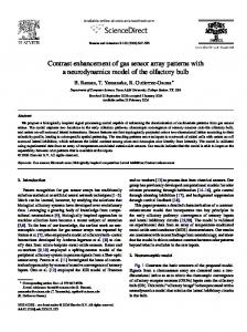
(b) Fig. 1. (a) Normalized conductance against hydrogen concentration, (b) Hysteresis cycle for methane (o: sensor TGS813, : sensor TGS815).
+
III. PATTERN RECOGNITION SYSTEM To succeed in gas classification, it is essential that every sensor exhibit a different pattern of sensitivities to the possible gas components. Moreover, the recognizer has to be robust against the usual problems for these sensors. Fig. 1 shows an example of their static characteristics: conductance against concentration for hydrogen. Maximum nonlinearities of the order of 20% full scale appear and maximum hysteresis of 5% full scale. In addition, we were looking for a fast and stable recognizer, so our system has to cope with the sensing dynamics. The sensor array system reacts slowly and takes some minutes to reach the stationary state. This time is a combination of the time to fill the chamber and the sensors time response. In addition, some of them do not achieve a constant value after a gas step, but show a maximum followed by a slow decay. All these problems result in a dispersion of the patterns produced by the feature extractor.
where is the sensor conductance. For nonlinear sensors this normalization does not cancel completely the concentration dependence, and there are several other possibilities. Some of them are listed in Table I. Even after this normalization, the clusters are far from the ideal situation due to this and other problems mentioned before: hysteresis, dynamic effects, drifts, etc. It is necessary to use a pattern recognition engine that separates the regions of the normalized data space as belonging to different gas classes. As it is impossible to observe the separation of the clusters in a six-dimensional space, we have decided to use principal component analysis [13] for visualization purposes, reducing the dimensionality to two. However, it is clear that due to the linearity of this technique, even clusters that appear confused in the 2-D projection may be separated by nonlinear techniques. We have chosen the SOM for this task. The SOM is an artificial neural net with the ability of creating a spatially organized representation (maps) of multiple features from input signals in an unsupervised manner, which resembles the cortices maps topographically organized in human brain [14]. The architecture consists of a single layer (rectangular shape) of neurons whose weights represent their position in the pattern space. During the training process, a representing a gas pattern vector from a training set
Authorized licensed use limited to: Universitat de Barcelona. Downloaded on February 16, 2009 at 06:54 from IEEE Xplore. Restrictions apply.
318
IEEE TRANSACTIONS ON INSTRUMENTATION AND MEASUREMENT, VOL. 47, NO. 1, FEBRUARY 1998
is presented to the net, the winning neuron (the closest to the pattern with a Euclidean metric) and its neighbors (the neighborhood area) change their position, becoming closer to the input pattern according to the following learning rule:
where are the weights of the neurons inside the neighborhood area, is the index of the neuron, is the index of the is the learning rate, pattern, is the time step, is the neighborhood function, and is the distance between the neuron and the winner measured over the net using a Manhattan metric. The learning rate and the neighborhood are monotonically decreasing functions along the training. When the training has converged, the net has learned the topology of the input patterns. In other words, neighbor neurons specialize in neighbor regions of the input space. Moreover, neurons cluster in the regions where the probability density function of the patterns is higher. Finally, it is necessary to have a supervised step to label the neurons. The training patterns are presented again to the net and the winning neuron is labeled with the class of input pattern. If conflicts appear, we have defined a criteria to solve them. First, the class that more frequently fires the neuron. If conflicts still persist, the labeling system decides upon the neighbors’ neurons label. During operation, the winning neuron determines the class attributed to the gas. IV. GAS CLASSIFIER DEFINITION
AND
+
Fig. 2. Polar representation of the patterns for CH4 (solid) and CH4 CO (dashed).
TEST
Although the architecture of the gas classifier has been outlined in the previous section, several details need further work: selection of the best neural net size, selection of the best data normalization, study of the dynamic effects, and methods of drift counteraction. We are going to describe first how the SOM training and recognizer test has been done. As is usual in these kinds of problems, the data set is divided in two parts. The first part is used to train the net, and the second part is used to test the net. Training patterns were chosen from different pulse concentrations and at different time points of the pulse response. A larger number of patterns have been selected from the extremes of the concentration range and from the initial part of the dynamic response to give a larger weight to the a priori more difficult cases. The validation patterns have been obtained among different concentrations and time points. During the classifier test, we have often found that a subset of sensors provides better results than the full set. In addition, this subset can be different depending on the chosen data normalization. The underlying reason can be seen looking at the patterns produced by each gas. From PCA plots, the main difficulties for classification are the detection of CO in the presence of CH , the detection of CO in the presence of H ,, and the detection of CO that is confused with air. We compare the patterns produced by these combinations and select those sensors whose outputs are maximally different. For instance, in Fig. 2 we show the patterns for CO and CH CO corresponding to normalization 1. It can be observed that if
Fig. 3. Pattern (dots) and neuron distribution (symbols) in the PCA projection after the SOM training. Normalization N1 and sensors: 23 456.
the presence of CO has to be detected in an atmosphere of CH , sensor six has to be included in the array. 8 map with 210 patterns (produced After training an 8 by the sensor subset 23 456 with normalization 1) the position of patterns and neurons are shown in Fig. 3 as a PCA projection. The results have been obtained with 315 patterns and are presented in Table I. Each cell within the table presents percentage of recognition, the classifier errors, and unclassified samples. These unclassified samples corresponds to the activation of neurons without an assigned label. In the best case, normalization N1 sensors 23456, success of 98.7% is achieved compared to 95.6% if all the sensors are used. The usual system errors are the undetection of CO in the presence
Authorized licensed use limited to: Universitat de Barcelona. Downloaded on February 16, 2009 at 06:54 from IEEE Xplore. Restrictions apply.
MARCO et al.: GAS IDENTIFICATION WITH TIN OXIDE SENSOR ARRAY AND SELF-ORGANIZING MAPS
TABLE II CLASSIFICATION SUCCESS DEPENDENCE ON NETWORK SIZE. SUCCESS, ERROR, AND UNCLASSIFICATION PERCENTAGE ARE SHOWN. BEST RESULTS ARE REMARKED
319
TABLE IV CLASSIFICATION SUCCESS ALONG TIMES. SUCCESS, ERROR, UNCLASSIFIED PERCENTAGE ARE SHOWN. BEST RESULTS ARE REMARKED
TABLE III CLASSIFICATION SUCCESS DEPENDENCE ON THE TRAINING SET SIZE. SUCCESS, ERROR, AND UNCLASSIFIED PERCENTAGE ARE SHOWN. BEST RESULTS ARE REMARKED
of hydrogen or methane, and the usual unclassification is the nonrecognition of air. Table I evidences the importance of choosing the right sensors and normalization procedure. To assure the goodness of the SOM, we tested the net size and the influence of the training and validation data set size. It is known that the number of neurons needed increases with the complexity of the pattern set statistics. From Table II we observe that the maximum in classification success is obtained for an 8 8 net. It may be inferred that there is an optimum number of neurons and it is unnecessary to increase the net size, as 64 neurons are enough to retain the statistics of the input space. About the training set size: one may expect that the efficiency of the SOM may improve with an increasing number of training patterns, but as shown in Table III, there is minimum number for succeeding. Furthermore, one additional goal is to reduce the training set as much as possible due to the high cost of the calibration data set. Regarding the validation set size, the increase from 315 to 525 patterns does not show significative changes. On the other hand, we have tested the influence of the sensor’s hysteresis on the system performance. This test has been carried out adding 25% of measurements from the decreasing concentration ramp in the validation set, resulting in minor differences (98.9% compared with the previous 98.7%). These results confirm the robustness of the recognizer. Concerning dynamic effects, one possible goal in pattern recognition is to achieve reliable results as fast as possible. In order to study the influence of time response in the success classification percentage, what we have done is to select patterns from different time points of the sensor responses and perform the validation on them. The selected patterns are classified in three groups: times lower than 3 min, times between 3 and 7 min, and times greater than 7 min (time referred to the rising edge of the concentration step). While the best results (normalization 1, sensors 23 456) have been obtained with times between 3 and 7 min (Table IV), it is remarkable that for times lower than 3 min, only a minor
decrease of classification performance has been found despite min) the system dynamics. Moreover, short term decays of the sensor response have also a minor influence. V. LONG-TERM DRIFT COMPENSATION Chemical sensors tend to show significant variations over long time periods when exposed to identical atmospheres. These drifts are due to the aging of the sensors, poisoning effects, and perhaps fluctuations in the sensor temperature due to environmental changes (usually sensors are operated without any control on the internal temperature). These longterm drifts produce dispersion in the patterns, and it can eventually change the cluster distribution in the data space, making useless the internal representation reached by the SOM net during the training phase. Compensation of these unpredictable drifts have only recently received some attention from the scientific community [15], [16]. To compensate the cluster’s movement due to sensor drifts, we propose to keep the SOM learning during the normal operation phase. However, during the operation, the learning rate has to be kept to a very low value, and in this phase the neighborhood extension has been reduced to zero: only the winning neuron adapts its weights. This is similar to the proposal in [15], but while in this paper the authors use only a neuron by gas class, we allow an arbitrary number within the SOM size and depending on the gas statistics. This added flexibility permits us to cope with more complex pattern distributions in the data space. Otherwise, with only one neuron per class, the cluster appearance is controlled by the used metric, while in our case it can be arbitrary. The efficiency of this proposal has been tested against sim, ulated drifts. They have been modeled as: is the sensor output before the drift experiment, and where has been chosen randomly for every sensor within the interval ( 0.4, 0.4). These extreme values are in order of the expected drifts for four year’s operation according Japanese
Authorized licensed use limited to: Universitat de Barcelona. Downloaded on February 16, 2009 at 06:54 from IEEE Xplore. Restrictions apply.
320
IEEE TRANSACTIONS ON INSTRUMENTATION AND MEASUREMENT, VOL. 47, NO. 1, FEBRUARY 1998
ACKNOWLEDGMENT The authors want to acknowledge to the group of Prof. W. G¨opel from the Institute of Physical and Theoretical Chemistry of the University of T¨ubingen, Germany, for measurements used in this work. REFERENCES
Fig. 4. Classification success against drift percentage.
gas sensor manufacturer FIS [17]. is the maximum number of time steps considered for the drift experiment: 6720. The learning rate was kept to 0.01. This value has to chosen as a tradeoff to permit adaptation but prevent the system from being oscillation prone. The system is tested for classification and with 168 success after patterns. First at all, we have studied the robustness of the SOM against these drifts when no adaptation is allowed: that is, with the static system. As expected, the success percentage declines, but it still remains higher than 80% for drifts up to 20%. In comparison, the adaptive net shows almost no success loss up to the same percentage and even then a less steep decay. Fig. 4 shows the comparison between both nets for a gas problem composed of four pure gases and two mixtures. The final decay is due to confusion in the data space among the different clusters. However, the final assessment of the success of our proposal has to wait till it is tested against real sensor’s drift data. VI. CONCLUSIONS From the presented results, we have succeeded in finding a method which is able to classify the gas with a very low error rate (