Gene ordering in partitive clustering using microarray expressions

Gene ordering in partitive clustering using microarray expressions

1019

Gene ordering in partitive clustering using microarray expressions SHUBHRA SANKAR RAY1,*, SANGHAMITRA BANDYOPADHYAY2 and SANKAR K PAL1 1

Center for Soft Computing Research: A National Facility, 2Machine Intelligence Unit, Indian Statistical Institute, Kolkata 700 108, India *Corresponding author (Fax, 91-33-2578 8699; Email, [email protected])

A central step in the analysis of gene expression data is the identification of groups of genes that exhibit similar expression patterns. Clustering and ordering the genes using gene expression data into homogeneous groups was shown to be useful in functional annotation, tissue classification, regulatory motif identification, and other applications. Although there is a rich literature on gene ordering in hierarchical clustering framework for gene expression analysis, there is no work addressing and evaluating the importance of gene ordering in partitive clustering framework, to the best knowledge of the authors. Outside the framework of hierarchical clustering, different gene ordering algorithms are applied on the whole data set, and the domain of partitive clustering is still unexplored with gene ordering approaches. A new hybrid method is proposed for ordering genes in each of the clusters obtained from partitive clustering solution, using microarray gene expressions. Two existing algorithms for optimally ordering cities in travelling salesman problem (TSP), namely, FRAG_GALK and Concorde, are hybridized individually with self organizing MAP to show the importance of gene ordering in partitive clustering framework. We validated our hybrid approach using yeast and fibroblast data and showed that our approach improves the result quality of partitive clustering solution, by identifying subclusters within big clusters, grouping functionally correlated genes within clusters, minimization of summation of gene expression distances, and the maximization of biological gene ordering using MIPS categorization. Moreover, the new hybrid approach, finds comparable or sometimes superior biological gene order in less computation time than those obtained by optimal leaf ordering in hierarchical clustering solution. Ray S S, Bandyopadhyay S and Pal S K 2007 Gene ordering in partitive clustering using microarray expressions; J. Biosci. 32 1019–1025]

1.

Introduction

The recent advances in DNA array technologies have resulted in a significant increase in the amount of genomic data. The most powerful and commonly used technique is that involving microarray, which has enabled the monitoring of the expression levels of more than thousands of genes simultaneously. A key step in the analysis of gene expression data is the identification of groups/clusters of genes that manifest similar expression patterns. This translates to the algorithmic problem of clustering and ordering of gene expression data. Keywords.

The present article deals with the tasks of ordering genes within clusters obtained from self-organizing map (SOM) (Tamayo et al 1999). Although there is a rich literature on gene ordering in hierarchical clustering framework (Eisen et al 1998; Biedl et al 2001; Bar-Joseph et al 2001), there is no work addressing and evaluating the importance of gene ordering for gene expression analysis in partitive clustering framework, to the best knowledge of the author. Partitive clustering methods determine unique clusters but do not order genes within cluster and the relationships among the genes in a particular cluster are generally lost. To obtain this relationship among genes in clusters, we propose a

Computational biology; evolutionary algorithms; genomics; linear programming; proteomics; soft computing

Abbreviations used: GA, genetic algorithm; MIPS, Munich Information for Protein Sequences; NF, nearest-neighbor; SOM, self-organizing map; TSP, traveling salesman problem http://www.ias.ac.in/jbiosci

J. Biosci. 32(5), August 2007, 1019–1025, © Indian Academy of Sciences 1019 J. Biosci. 32(5), August 2007

Shubhra Sankar Ray, Sanghamitra Bandyopadhyay and Sankar K Pal

1020

novel hybrid method where, an existing pure gene ordering algorithm called “FRAG_GALK” (Ray et al 2007), is used to order genes in each clustering solution of SOM (Tamayo et al 1999). For the purpose of comparison, instead of FRAG_GALK, an existing traveling salesman problem (TSP) solver Concorde (Applegate et al 2003) using linear programming, and optimal leaf ordering in hierarchical clustering solution (applied over the whole data set not partitive clustering solution) by Bar-Joseph et al (2001), are also used. Utility of the new hybrid algorithm is shown in improving the quality of the clusters provided by any partitive clustering algorithm by, • • • •

identification of subclusters within big clusters, grouping functionally correlated genes within clusters, the maximization of biological gene ordering using MIPS categorization, and using less computation time than those obtained by optimal leaf ordering in hierarchical clustering solution. 2.

Existing approaches

2.1

Distance measure

The most popular and probably most simple measures for finding global similarity between genes are the Pearson correlation, a statistical measure of linear dependence between random variables. Let X=x1, x2, … , xk and Y=y1, y2, … , yk be the expression vectors of the two genes in terms of log-transformed microarray gene expression data obtained over a series of k experiments. Using Pearson correlation the distance between gene X and Y can be formulated as Cx,y = 1 – Px,y ,

(1)

where Px,y represents the centered Pearson correlation and is defined as Px , y =

1 k ⎛⎜ xi − X ⎞⎟⎛⎜ yi − Y ⎞⎟⎟ ⎟⎜ ⎟, ∑⎜ k i=1 ⎜⎝ σ x ⎟⎟⎠⎜⎜⎝ σ y ⎟⎠

(2)

where X and σx are the mean and standard deviation of the gene X, respectively. 2.2

Gene ordering methods

Hierarchical clustering does not determine unique clusters. Thus the user has to determine which of the subtrees are clusters and which subtrees are only a part of a bigger cluster. So in the framework of hierarchical clustering a gene ordering algorithm helps the user to identify clusters J. Biosci. 32(5), August 2007

by means of visual display and interpret the data (Bar-Joseph et al 2001), whereas, in partitive clustering clusters are identified by the algorithm automatically and the solutions are robust and not sensible to noise (Tamayo et al 1999) like hierarchical clustering. For partitive clustering based approaches as well as for hierarchical clustering approaches microarray gene ordering (MGO) within clusters using gene expression information is necessary for the following reasons: (i)

Gene ordering helps to identify subclusters in big clusters by means of visual inspection of the ordered gene expression data (Bar-Joseph et al 2001). (ii) Genes that are adjacent in a linear ordering are often functionally co-regulated and involved in the same cellular process (Bar-Joseph et al 2001). Biological analysis is often done in the context of this linear ordering. (iii) The relationships among the genes in a particular cluster generated by partitive clustering algorithms are generally lost. This relationship (closer or distant) among genes within clusters can be obtained using gene ordering approaches. (iv) It provides smooth display of clustered genes, where the functionally related genes are nearer in the ordering. Ideally, one would like to obtain a linear order of all genes that puts similar genes close to each other; such that for any two consecutive genes the distance between them is small. So, gene ordering problem is similar to TSP (Pal et al 2006) where, cities are ordered instead of genes (Biedl et al 2001; Ray et al 2007; Tsai et al 2004). Let {1,2, … , n} be the labels of the n cities and C = [ci,j] be an n × n distance matrix where ci,j denotes the distance of traveling from city i to city j. The TSP is the problem of finding the shortest closed route among n cities, having as input the complete distance matrix among all cities. The total cost A of a TSP tour is given by n −1

A(n) = ∑ Ci ,i +1 + Cn ,1.

(3)

i =1

The objective is to find a permutation of the n cities, which has minimum distance. Similarly, an optimal gene order can be obtained by minimizing the summation of gene expression distances (or maximizing summation of gene expression similarities) between pairs of adjacent genes in a linear ordering 1,2,..., n. This can be formulated as (Biedl et al 2001) n −1

F (n) = ∑ Ci ,i +1 ,

(4)

i =1

where n is the number of genes and ci,j+1 is the distance/ similarity between two genes i and i + 1 obtained from

Gene ordering in partitive clustering using microarray expressions distance/similarity matrix. The formula (eq. 4) for optimal gene ordering is the same as used in TSP, except the distance from the last gene to first gene, which is omitted, as the tour is not a circular one. In the related investigations, FRAG_GALK (Ray et al 2007) and HeSGA (heterogeneous selection genetic algorithm (Tsai et al 2004), was applied to order genes of the whole dataset, and consequently clustering information was missing from the ordering solution. A method of ordering genes for a partitive clustering solution is currently missing. Here, we define the summation of gene expression distances for a partitive clustering solution as k

n j −1

F1 (n) = ∑ ∑ C j =1 i =1

j i ,i +1

,

Step 5: Using the evaluated fitness of entire population, linear normalized selection procedure is used. Step 6: Chromosomes are now distributed randomly and modified order crossover operator is applied between two consecutive chromosomes probabilistically. Step 7: Simple inversion mutation (SIM) is performed on each string probabilistically. Step 8: Generation count of GA is incremented and if it is less than the maximum number of generations (predefined) then from step 2 to step 6 are repeated.

(5)

where k is the total number of clusters, nj is the number of j genes in cluster j, and C i,j+1 is the distance/similarity between two genes i and i + 1 in cluster j. In this investigation we have used two different gene ordering algorithms, FRAG_GALK (Ray et al 2007) and Concorde’s TSP solver (Applegate et al 2003), to order genes of individual clusters found by SOM, as they can obtain the optimal order of cities to many of the TSPLIB instances; the largest having 13,509 and 15,112 cities, respectively. While FRAG_GALK is a genetic algorithm (GA) (Pal et al 2006) based TSP solver, Concorde is a linear programming based TSP solver and much slower than FRAG_GALK. Here we briefly discuss the various steps used in FRAG_GALK, which are also available in Ray et al (2007). The steps are: Step 1: Create the string representation (chromosome of GA) for a gene order (an array of n integers), which is a permutation of 1, 2, ······ , n with nearest-neighbor (NF) heuristic. Repeat this step to form the initial population of GA. Step 2: The NF heuristic is applied on each chromosome probabilistically. Step 3: Each chromosome is upgraded to local optimal solution using chained LK heuristic (Applegate et al 2003) probabilistically. Step 4: Fitness of the entire population is evaluated and elitism is used, so that the fittest string among the child population and the parent population is passed into the child population.

1021

3.

Materials and methods

3.1

Description of data sets

In the present investigation, data sets like cell cycle (Sherlock et al 2001), yeast complex (Eisen et al 1998; Bar-Joseph et al 2001), all yeast (Eisen et al 1998; Website: Eisenlab: http://rana.lbl.gov./EisenData.htm) and fibroblast (Iyer et al 1999) are chosen. Table 1 shows the name of the data sets, number of genes in each dataset, number of biological gene categories, name of experiment types and number of time points under each type, and finally the total number of time points for a particular dataset. The first three data sets of Saccharomyces cerevisiae consist of 652, 979 and 6221 genes, and 184, 79 and 80 time points, respectively. The genes in the three data sets are classified according to the top level classification (hierarchical structure) of Munich Information for Protein Sequences (MIPS) (http://www.mips.com) into 16, 16, and 18 categories, respectively. For the cell cycle data, first we have downloaded 652 cell cycle regulated gene names from the MIPS website. These gene names are then uploaded in Stanford Microarray Database (Sherlock et al 2001) and corresponding gene expression values are downloaded with default parameters by selecting all the cell cycle, sporulation, heat shock and diauxic shift experiments. The fibroblast dataset consists of 517 genes and 18 time points related to the response of human fibroblasts to serum. According to gene omnibus (GO) annotation, 517 fibroblast genes are distributed in 1347 categories. After downloading, the order of genes (along with their expression vectors) is randomized in each dataset to remove initial gene order bias.

Table 1. Summary for different microarray data sets Dataset

No. of genes Category

Experiments performed

Total

Cell cycle

652

MIPS 16

Cell cycle 93

Sporulation 9

Shock 56

Diauxic shift 26

184

Yeast complex

979

MIPS 16

Cell cycle 18+14+15

Sporulation 7+4

Shock 6+4+4

Diauxic shift 7

79

All yeast

6221

MIPS 18

Cell cycle 60

Sporulation 13

Diauxic shift 7

Fibroblast

517

GO 1347

Serum response 12

Cycloheximide 6

80 18

J. Biosci. 32(5), August 2007

Shubhra Sankar Ray, Sanghamitra Bandyopadhyay and Sankar K Pal

1022 3.2

New hybrid algorithm for ordering genes in partitive clustering

It is mentioned in § 2.2 that, FRAG_GALK is applied separately on each of the gene clusters found by SOM to identify subclusters within large clusters, and to group the functionally correlated genes within clusters. The number of nodes/clusters of SOM are chosen according to the number of MIPS categories (top level of hierarchical tree) for yeast data, and available information in Sharan et al (2003) for fibroblast data. 4.

Biological interpretation

In case of cell cycle, yeast complex, and all yeast data the MIPS functional categorization is available for most of the genes. The categorization is hierarchical in nature and allows a gene to belong to more than one category. A biological score, that is different from the similarity/distance measures, is used to evaluate the final gene ordering. Each gene that has undergone MIPS categorization can belong to one or more category, while there are many unclassified genes also (no category). A vector V(g) = (ν1, ν2, … , νj) is used to represent the category status of each gene g, where j is the number of categories. The value of νj is 1 if gene g is in the jth category; otherwise is zero. Based on the information about categorization, the score of a gene order for multiple class genes is defined as (Tsai et al 2004) N −1

S (n) = ∑ G (gi , gi +1 ),

(6)

i =1

where N is the number of genes, gi and gi+1 are the adjacent genes and G(gi, gi+1) is defined as j

G (gi , gi +1 ) = ∑ V ( gi ) k V (gi +1 )k ,

(7)

k =1

where V(gi)k represents the kth entry of vector V(gi). For example consider the genes g1, g2, … , g5, which are classified into 15 categories and represented by the following vectors: V(g1) = (1,0,1,1,0,0,0,0,0,0,0,0,0,0,0) V(g2) = (1,1,1,1,0,0,0,0,0,0,0,0,0,0,0) V(g3) = (0,0,1,0,0,0,0,0,1,0,0,0,0,0,0) V(g4) = (0,0,0,1,1,0,0,0,0,1,0,0,0,0,0) and V(g5) = (0,0,0,0,1,0,0,0,0,1,0,0,0,0,0). Considering the gene order g1,g2,g3,g4,g5, G(g,g2) = 3, G(g2,g5) = 1, G(g3,g4) = 0, G(g4,g5) = 2, and S(n) = G(g1,g2) + G(g2,g3)+ G(g3,g4)+ G(g4,g5) =3+1+0+2=6 J. Biosci. 32(5), August 2007

Using scoring function S(n), a gene ordering would have a higher score when more genes within the same group are aligned next to each other. So higher values of S(n) are better and can be used to evaluate the goodness of a particular gene order. 5.

Experimental results

Experiments of gene ordering are conducted in Matlab 7 on Sun Fire V 890 (1.2 GHz and 8 GB RAM). The codes for BarJoseph et al’s (2001) leaf ordering in hierarchical clustering solution are downloaded from (Venet 2003). Performance of the proposed FRAG_GALK for gene ordering is compared mainly with Concorde’s linear programming algorithm and Bar-Joseph et al’s method. SOM is available in Expander (Sharan et al 2003) and used with 16, 16, and 18 clusters for clustering cell cycle, yeast complex, and all yeast data sets, respectively, as genes in these datasets are classified according to MIPS into 16, 16, and 18 functional categories. For fibroblast data SOM is used with 6 clusters as 6 gene clusters are identified in Sharan et al (2003). Finally FRAG_ GALK and Concorde are applied separately on the gene clusters obtained by SOM, and Bar-Joseph et al’s method is applied on the average linkage based hierarchical clustering solution for each dataset. 5.1

Relevance of gene ordering in partitive clustering

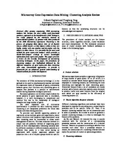
To show the utility of the hybrid method in identifying different subclusters within big clusters and grouping the functionally correlated genes within clusters, here for illustration, the visual displays are presented for fibroblast (Figure 1a, b) and yeast complex (Figure 1c, d) data. Using SOM fibroblast genes are first clustered in 6 clusters (stated previously). Visual display of these 6 clusters is shown in figure 1a. Observing this visual pattern no subcluster can be identified in each cluster. After applying FRAG_GALK on each cluster, closely related genes with similar expressions are aligned next to each other as shown in Figure 1b. Gene ordering here suggests that 2 or more subclusters exists at least in clusters 1, 4 and 6, and it will be useful to increase the number of nodes of SOM to at least 9 for fibroblast data. Note that, Iyer et al (1999) identified 10 clusters of genes for this data using average linkage clustering. Yeast Complex data is first clustered in 16 groups using SOM. Visual display of first 6 clusters/groups is shown in figure 1c. When the genes are ordered in each cluster with FRAG_GALK, 4, 4, 5, and 2 distinct subclusters are identified using visual display in clusters 2, 3, 4, and 5 respectively. Genes names along with their functional categories (indexes) for each subcluster within cluster 4 are shown in table 2 for the purpose of illustration. Names of

Gene ordering in partitive clustering using microarray expressions

(a)

(b)

1023

(c)

(d)

Figure 1. Comparing SOM with ‘SOM+FRAG_GALK’ for Fibroblast data (a and b respectively) and Yeast Complex data (c and d respectively). The expression profiles are represented as lines of coloured boxes using Expander (Sharan et al 2003), each of which corresponds to a single experiment. Table 2. Gene subclusters found by SOM+FRAG_GALK and their functional category indexes in cluster 4 for yeast complex data Cluster

Subcluster

Genes

Functional index

4

1

YLR093C, YNL121C, YLR170C, YML112W, YBR160W, YBR171W, YLR378C, YML019W, YPL234C, YOR039W

6

2

YKR068C, YLL050C, YGL200C, YML012W, YPL218W, YKL080W, YDR086C, YNL153C, YKL122C, YLR292C, YGL112C, YLR268W YLR447C

6 and 9

3

YBR010W, YNL031C, YBL003C, YDR225W, YDR224C, YNL030W, YBR009C, YBL002W, YPL256C

3, 4, and 7

4

YJL025W, YPR101W, YMR061W, YGR195W, YOR244W, YLR105C, YDL043C, YPR056W, YPR057W

4

5

YGL100W, YNL261W, YKL144C, YNL151C, YJL008C, YER148W

7

the functional categories corresponding to their indexes are shown in table 3. These subclusters of highly coregulated genes cannot be identified if SOM is used alone. For example, all the 9 genes in the 3rd subcluster of cluster 4 (YBR010W, YNL031C, YBL003C, YDR225W, YDR224C, YNL030W, YBR009C, YBL002W and YPL256C) are involved in cell cycle and DNA processing, transcription, and protein with binding function or cofactor requirement. While using SOM these 9 genes are distributed in the cluster 4, after ordering genes in cluster 4 of SOM with FRAG_GALK, they (the 9 genes) are tightly grouped and identified easily using visual display. With all these ordered and clustered genes one can easily zoom in a useful small subset of genes in a

cluster which cannot be done alone with partitive clustering methods. In a similar way, subclusters within big clusters are identified by Concorde for all the data sets. 5.2

Comparative Performance of Algorithms

The ultimate goal of an ordering algorithm is to order the genes in a way that is biologically meaningful. In this regard, table 4 compares the performance of our proposed two hybrid approaches using FRAG_GALK and Concorde with Bar-Joseph’s (Bar-Joseph et al 2001) leaf ordering in hierarchical clustering solution in terms of the F1 value J. Biosci. 32(5), August 2007

Shubhra Sankar Ray, Sanghamitra Bandyopadhyay and Sankar K Pal

1024

Table 3. Indexes and corresponding functional category Functional index

Corresponding functional category

1

Metabolism

2

Energy

3

Cell cycle and DNA processing

4

Transcription

5

Protein synthesis

6

Protein fate (folding, modification, destination)

7

Protein with binding function or cofactor requirement

8

Protein activity regulation

9

Cellular transport, transport facilitation and transport routes

Table 4. Summation of gene expression distances (F1), biological score (S), and computation time of ordering in seconds (within parenthesis) for different algorithms Data sets Algorithm

Cell cycle

Yeast complex

All yeast

SOM

442.94 354

547.16 792

3446.60 1730

SOM +FRAG_ 301.72 GALK 386 (0.7)

330.54 1011 (1.13)

1919.15 2356 (125)

SOM +concorde

301.72 386 (3.41)

330.54 1011 (15.26)

1919.15 2356 (2272)

Bar-Joseph

300.51 381 (1.8)

330.17 1024 (3.34)

1920.82 2350 (1989)

(eq. 5), S value (eq. 6), and computation time. The performance of an algorithm is better if F1 value is smaller and S value is larger. For Fibroblast data, no biological score is provided as genes in the same biological group for this data are rare. From the biological scores (table 4), it is evident that FRAG_GALK provides biologically comparable gene order with respect to Concorde and sometimes superior gene order than ‘leaf ordering in hierarchical clustering solution’ by Bar-Joseph et al (2001), for all datasets in least computational time. For example, FRAG_GALK took 125 seconds to order all yeast data (6221 genes) as compared to Concorde and Bar-Joseph et al’s method which took 2272 and 1989 seconds respectively. 6.

Conclusion

A hybrid method of gene ordering in partitive clustering and its utility in finding useful subgroups of genes within cluster, grouping functionally correlated genes within clusters, maximization of biological gene ordering using MIPS categorization, and minimization of computation time, are J. Biosci. 32(5), August 2007

demonstrated. The hybrid approach not only determines unique clusters, but also preserves the biologically meaningful relationships among the genes within clusters. Moreover, the hybrid method using SOM with FRAG_ GALK not only requires less computation time (125 s for 18 clusters of all yeast data) but also less amount of RAM (0.1 GB RAM for clusters with 1000 genes) than original Bar-Joseph’s method (1989 s and 2 GB RAM for all yeast data). With the hybrid approaches one can easily zoom in a useful small subset of genes in a cluster, which cannot be done alone with partitive clustering methods. In FRAG_GALK, parallel searching (with large population in genetic algorithm) for optimal gene order in gene clusters (closely related genes) is performed. While this results in reduced searching time for FRAG_GALK than Concorde and Bar-Joseph’s method, in terms of biological score FRAG_GALK is comparable with Concorde and sometimes superior to Bar-Joseph’s method. It is evident from the experimental results that, the combination of partitive clustering and FRAG_GALK is a promising tool for microarray gene expression analysis. References Applegate D, Bixby R, Chvtal V and Cook W 2003 Concorde Package. [Online], www.tsp.gatech.edu/concorde/downloads/ codes/src/co031219.tgz Bar-Joseph Z, Gifford D K and Jaakkola T S 2001 Fast optimal leaf ordering for hierarchical clustering; Bioinformatics 17 2229 Biedl T, Brejov B, Demaine E D, Hamel A M and Vinar T 2001 Optimal arrangement of leaves in the tree representing hierarchical clustering of gene expression data (Technical report, Department of Computer Sciemce, University of Waterloo) Eisen M B, Spellman P T, Brown P O and Botstein D 1998 Cluster analysis and display of genome-wide expression patterns; Proc. Natl Acad. Sci., USA 95 14863–14868 Iyer V R, Eisen M B, Ross D T, Schuler G, Moore T, Lee J C F, Trent J M, Staudt L M et al 1999 The transcriptional program in the response of human fibroblasts to serum; Science 283 83–87 Pal S K, Bandyopadhyay S and Ray S S 2006 Evolutionary computation in bioinformatics: A review; IEEE Trans. Systems Man Cybernetics Part C 36 601–615 Ray S S, Bandyopadhyay S and Pal S K 2007 Genetic operators for combinatorial optimization in TSP and microarray gene ordering; Appl. Intelligence 26 183–195 Sharan R, Maron-Katz A and Shamir R 2003 CLICK and EXPANDER: a system for clustering and visualizing gene expression data; Bioinformatics 19 1787–1799 Sherlock G, Hernandez-Boussard T, Kasarskis A, Binkley G, Matese J C, Dwight S S, Kaloper M, Weng S et al 2001 The Stanford microarray database; Nucleic Acids Res. 29 152–155

Gene ordering in partitive clustering using microarray expressions Tamayo P, Slonim D, Mesirov J, Zhu Q, Kitareewan S, Dmitrovsky E, Lander E S and Golub T R 1999 Interpreting patterns of gene expression with self-organizing maps: Methods and application to hematopoietic differentiation; Proc. Natl. Acad. Sci. USA 96 2907–2912

1025

Tsai H K, Yang J M, Tsai Y F and Kao C Y 2004 An evolutionary approach for gene expression patterns; IEEE Trans. Info. Tech. Biomed. 8 69–78 Venet D 2003 MatArray: a Matlab toolbox for microarray data; Bioinformatics 19 659–660

ePublication: 28 June 2007

J. Biosci. 32(5), August 2007