Home
Search
Collections
Journals
About
Contact us
My IOPscience
Generalized PSF modeling for optimized quantitation in PET imaging
This content has been downloaded from IOPscience. Please scroll down to see the full text. 2017 Phys. Med. Biol. 62 5149 (http://iopscience.iop.org/0031-9155/62/12/5149) View the table of contents for this issue, or go to the journal homepage for more Download details: IP Address: 162.129.251.29 This content was downloaded on 19/06/2017 at 20:08 Please note that terms and conditions apply.
You may also be interested in: Single scan parameterization of space-variant point spread functions F A Kotasidis, J C Matthews, G I Angelis et al. Noise and signal properties in PSF-based fully 3D PET image reconstruction S Tong, A M Alessio and P E Kinahan Non-Gaussian space-variant resolution modelling for list-mode reconstruction C Cloquet, F C Sureau, M Defrise et al. Applications of the line-of-response probability density function resolution model in PET list mode reconstruction Y Jian, R Yao, T Mulnix et al. A review of partial volume correction techniques for emission tomography and their applications in neurology, cardiology and oncology Kjell Erlandsson, Irène Buvat, P Hendrik Pretorius et al. Analytic System Matrix Resolution Modeling in PET A Rahmim, J Tang, M A Lodge et al. Noise propagation in resolution modeled PET imaging and its impact on detectability Arman Rahmim and Jing Tang A method for accurate modelling of the crystal response function S Stute, D Benoit, A Martineau et al. Bias in iterative reconstruction M D Walker, M-C Asselin, P J Julyan et al.
Institute of Physics and Engineering in Medicine Phys. Med. Biol. 62 (2017) 5149–5179
Physics in Medicine & Biology https://doi.org/10.1088/1361-6560/aa6911
Generalized PSF modeling for optimized quantitation in PET imaging Saeed Ashrafinia1,2, Hassan Mohy-ud-Din3, Nicolas A Karakatsanis4, Abhinav K Jha2, Michael E Casey5, Dan J Kadrmas6 and Arman Rahmim1,2 1
Department of Electrical and Computer Engineering, Whiting School of Engineering, Johns Hopkins University, Baltimore, MD, United States of America 2 Department of Radiology and Radiological Sciences, School of Medicine, Johns Hopkins University, Baltimore, MD, United States of America 3 Department of Radiology and Biomedical Imaging, Yale University, New Haven, CT, United States of America 4 Translational and Molecular Imaging Institute, Icahn School of Medicine at Mount Sinai, New York, NY, United States of America 5 Siemens Medical Systems, Knoxville, TN, United States of America 6 Department of Radiology, University of Utah, Salt Lake City, UT, United States of America E-mail:
[email protected] and
[email protected] Received 7 September 2016, revised 11 February 2017 Accepted for publication 24 March 2017 Published 26 May 2017 Abstract
Point-spread function (PSF) modeling offers the ability to account for resolution degrading phenomena within the PET image generation framework. PSF modeling improves resolution and enhances contrast, but at the same time significantly alters image noise properties and induces edge overshoot effect. Thus, studying the effect of PSF modeling on quantitation task performance can be very important. Frameworks explored in the past involved a dichotomy of PSF versus no-PSF modeling. By contrast, the present work focuses on quantitative performance evaluation of standard uptake value (SUV) PET images, while incorporating a wide spectrum of PSF models, including those that under- and over-estimate the true PSF, for the potential of enhanced quantitation of SUVs. The developed framework first analytically models the true PSF, considering a range of resolution degradation phenomena (including photon non-collinearity, inter-crystal penetration and scattering) as present in data acquisitions with modern commercial PET systems. In the context of oncologic liver FDG PET imaging, we generated 200 noisy datasets per image-set (with clinically realistic noise levels) using an XCAT anthropomorphic phantom with liver tumours of varying sizes. These were subsequently reconstructed using the OS-EM algorithm with 1361-6560/17/125149+31$33.00 © 2017 Institute of Physics and Engineering in Medicine Printed in the UK
5149
S Ashrafinia et al
Phys. Med. Biol. 62 (2017) 5149
varying PSF modelled kernels. We focused on quantitation of both SUVmean and SUVmax, including assessment of contrast recovery coefficients, as well as noise-bias characteristics (including both image roughness and coefficient of-variability), for different tumours/iterations/PSF kernels. It was observed that overestimated PSF yielded more accurate contrast recovery for a range of tumours, and typically improved quantitative performance. For a clinically reasonable number of iterations, edge enhancement due to PSF modeling (especially due to over-estimated PSF) was in fact seen to lower SUVmean bias in small tumours. Overall, the results indicate that exactly matched PSF modeling does not offer optimized PET quantitation, and that PSF overestimation may provide enhanced SUV quantitation. Furthermore, generalized PSF modeling may provide a valuable approach for quantitative tasks such as treatment-response assessment and prognostication. Keywords: PET, quantitation, standard uptake value (SUV), PSF modeling, partial volume correction (Some figures may appear in colour only in the online journal) 1. Introduction PET imaging is affected by a number of resolution degrading factors that result in undesirable cross-contamination between adjacent voxel regions, referred to as the partial volume effect (PVE) (Soret et al 2007, Rahmim and Zaidi 2008). This issue has been tackled via a number of partial volume correction (PVC) methods that aim to improve image quantitation (Erlandsson et al 2012). However, these techniques often involve simplifying assumptions, require access to well-registered anatomical (e.g. MRI, CT) images, and can amplify noise levels (Muller-Gartner et al 1992, Rousset et al 1998, 2007, 2008). A distinct approach to this problem is point-spread function (PSF) modeling, also referred to as resolution modeling (RM). PSF modeling aims to capture and correct for object-domain and/or detection-domain resolution degrading effects to facilitate more accurate modeling of the measurement (Iriarte et al 2016). It therefore reduces image degradations caused by model-mismatch and yields improvements in reconstructed image quality as it compensates for some partial volume effects. As such, PSF modeling has attracted considerable interest in PET over the past decade (Rahmim et al 2013, Iriarte et al 2016), and has been adopted by major PET vendors in their state-of-the-art PET scanners (Rapisarda et al 2010, Jakoby et al 2011, Miller et al 2015, Qi et al 2015, Slomka et al 2016). PSF modeling implementations are commonly divided into (i) image-space, and (ii) projection-space methods. Theoretical analysis of these two approaches has been provided (Cloquet et al 2010, Rahmim et al 2013), and a few studies have performed preliminary comparison between the two (Sureau et al 2008, Kotasidis et al 2011). Image-based methods attempt to incorporate resolution blurring effects entirely in the image-space, based on the idea that the reconstructed image can be considered as the blurring of the true image by a point-spread function. This can be performed within the image reconstruction (PSF modeling in the imagespace component of the system matrix, thus applied before forward projection and after back projection operations), or performed post-reconstruction in the form of iterative deconvolution (Reader et al 2003, Rahmim et al 2003, Antich et al 2005, Teo et al 2007, Cloquet et al 2010, Rapisarda et al 2010, Kotasidis et al 2011, Iriarte et al 2016). These methods are straightforward to implement, do not impose a significant computational burden, and produce images 5150
S Ashrafinia et al
Phys. Med. Biol. 62 (2017) 5149
with high quality, so that certain vendor PET scanners have already providing this option (Miller et al 2015). On the other hand, projection-space methods model degradation effects within the projection-space component of the system matrix. Recently, Iriarte et al published a review on system models for statistical reconstruction of PET data. They indicate that the most popular approach of combining models of physical degradation factors is to factor the system matrix as a product of independent matrices, each one describing one or a collection of effects (Iriarte et al 2016). This arrangement is a well-established approach that has led to high quality efficient reconstructions and yields substantial enhancements in storage preserving and computational time. Also, some studies on image-based PSF modeling considered anisotropy (Rahmim et al 2003, Antich et al 2005, Sureau et al 2008, Rapisarda et al 2010), using more complex functions, e.g. mixtures of Gaussians and exponential (Antich et al 2005, Sureau et al 2008, Cloquet et al 2010), and PSF estimation methods based on measurements of arrays of point sources (Sureau et al 2008, Kotasidis et al 2011, Kotasidis et al 2014). The projection-based methods can be categorized into: (a) empirical methods utilizing measured data points (Panin et al 2006a, 2006b), (b) Monte Carlo simulations (Mumcuoglu et al 1996, Qi et al 1998a, 1998b, Alessio et al 2006, Iriarte et al 2016), (c) analytical models (Lecomte et al 1984, Schmitt et al 1988, Selivanov et al 2000, Strul et al 2003, Rahmim et al 2008c) including additional modeling for positron range (Bai et al 2003, Bai et al 2005, Ruangma et al 2006, Rahmim et al 2008b, Alessio and MacDonald 2008), and (d) hybrid approaches incorporating combinations of these methodologies; e.g. starting with a simple geometrical calculation, and then imposing additional effects (Selivanov et al 2000, Carson et al 2003, Yamaya et al 2005, Takahashi et al 2007). These studies focus on benefits of different methodologies and exploit their synergies to compute the system matrix (Iriarte et al 2016). PSF modeling provides a number of advantages: (i) improved spatial resolution and contrast recovery (Reader et al 2003, Rahmim et al 2008b, Sureau et al 2008, Alessio et al 2010, Rapisarda et al 2010, Kotasidis et al 2011); (ii) reduced spatial noise or image roughness (IR), resulting in a visually smoother image (Vercher-Conejero et al 2013), and (iii) improved focal lesion detectability performance (Tong et al 2010, Rahmim and Tang 2013a, Karakatsanis et al 2014, 2015). At the same time, PSF modeling poses two concerns (Alessio et al 2013): First, it impacts noise characteristics of the reconstructed images as they appear smoother. Moreover, the resulting noise power spectrum (NPS) of the PSF modelled reconstructed image is seen to be amplified in the mid-frequency domain, while exhibiting smaller values at higher frequencies (Rahmim and Tang 2013b). Some efforts have been devoted to the analysis of the resulting noise properties that have important implications for quantitation and lesion detectability performance in PET imaging. These studies performed experimental evaluation of noise characteristics on real datasets (Boellaard et al 2004, Bernardi et al 2007, Kadrmas et al 2009, Rahmim and Tang 2013b), or through Monte Carlo simulations (Soares et al 2000, Soares et al 2005), and subsequently analysed the impact of reconstruction parameters by adopting a variety of figures-of-merit (FOMs). PSF modeling has different effects on different noise metrics (Tong et al 2010, Rahmim and Tang 2013b). Rahmim et al used analytic models of noise propagation (Barrett et al 1994, Wilson et al 1994) to investigate the impact with and without PSF modeling. In a PSF modelled system matrix, more lines-of-response (LORs) contribute to a single voxel, as each voxel is related to more measurement locations compared to a non-PSF modelled system. This results in a more ill-conditioned inverse problem that suffers from slow convergence (Tong et al 2011). Moreover, at matched iterations, voxels in a PSF reconstruction depict lower voxel variance and higher inter-voxel correlations versus no-PSF (Rahmim et al 2005, Tong et al 2010). As a result, PSF modeling noticeably alters the 5151
S Ashrafinia et al
Phys. Med. Biol. 62 (2017) 5149
noise texture. Tong et al derived analytical expressions relating image roughness and ensemble noise to voxel variance and inter-voxel correlations (Tong et al 2010). Due to PSF modeling, images become smoother, but the ensemble standard deviation of ROI mean uptake (a measure of reproducibility) may remain unchanged (Tong et al 2010) or even be amplified for smaller ROIs (Hoetjes et al 2010, Blinder et al 2012). We elaborate more on how this impacts different noise metrics in section 2. The second issue concerning PSF modeling is its susceptibility to produce edge overshoot effect—a reminiscence of Gibbs ringing patterns at the edges of a region (Snyder et al 1987, Politte and Snyder 1988, Tong et al 2011), manifesting as overshoots in smaller regions. This issue may compromise the accuracy of signal quantitation in small regions (Rahmim et al 2013). Snyder suggested using a less blurred (i.e. underestimated) version of the true PSF in the reconstruction (Snyder et al 1987, Politte and Snyder 1988). This method was shown to be effective at suppressing the edge overshoot effect (Tong et al 2011, Blinder et al 2012). Snyder (1987) also suggested that a possible reason for the appearance of edge overshoots is the mismatch between estimated PSF and true PSF, and that the small mismatch can be amplified due to the instability of deconvolution process. Nonetheless, it was shown (Reader et al 2003, Tong et al 2011, Ashrafinia et al 2014a, 2014b)—as we also demonstrate in this work— that even reconstruction with the true PSF results in the edge overshoot effect. Furthermore, for specific detection or quantitation tasks, it is plausible that such an effect may even enhance task performance, as we show in this work for quantitation. Finally, it is worth noting that clinical tasks vary from pure detection-related tasks (e.g. diagnosis and staging) to quantitation-related tasks (e.g. therapy response assessment and prognostication). The features that make a PET image suitable for detection task differ from those that make an image effective for tumour quantitation. In fact, noise contributes differently to these two general tasks, and PSF-induced noise propagation can result in improved quantitation but may reduce lesion detectability performance, or vice versa (Rahmim and Tang 2013b). However, such analyses and optimizations have only been performed for the case of no-PSF versus PSF modeling. It is possible to generalize PSF modeling to include overestimated and underestimated PSF kernels. This provides a wider range of options to study the impact of PSF modeling on quantitation tasks, thus facilitating task-based optim ization for quantitation. Furthermore, given the aforementioned challenges with reproducibility as well as edge overshoots in PSF modeling, it is plausible that generalized PSF modeling may provide kernels that perform optimally, properly balancing different effects. The present work pursues such a generalized PSF framework in the context of tumour quantitation, which in future efforts can be thoroughly evaluated for lesion detectability tasks as well. 2. Methods In this section, we describe our proposed approach to incorporate and assess generalized PSF kernels in the image reconstruction framework. First, we describe simulation configuration, followed by the image reconstruction method incorporating the true PSF kernel. We then explain the methodology of generating a spectrum of PSF kernels from the true PSF. Finally, we define the FOMs for assessing and analysing the results. 2.1. Simulation and phantom configuration
We used the 4D anthropomorphic XCAT phantom (Segars et al 2010) to generate dynamic FDGPET images of different tumours, as well as the corresponding attenuation map. In this study, we chose to implement six liver tumours of different diameters (10, 13, 17, 22, 28 and 37 mm), 5152
S Ashrafinia et al
Phys. Med. Biol. 62 (2017) 5149
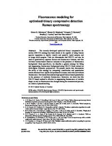
Figure 1. XCAT generated phantom as reference images with liver tumour sizes of (left) 10 mm, and (right) 22 mm. (a) Reference image, tumor diam.: 10 mm. (b) Reference image, tumor diam.: 22 mm.
which was in agreement with the NEMA NU-2 image quality phantom (NEMA 2012). The position of the centre of the tumour spheres is fixed across all six images for consistency. Figure 1 depicts two of these six reference images. The original reference image has a transaxial dimension of 1024 × 1024 and a voxel size of 0.5856 mm, and 2D OS-EM reconstructions with seven subsets are performed into 256 × 256 images with voxel dimensions 3.47 × 3.47 × 3.27 mm3. Starting from a higher resolution image is more realistic to better capture the spatial continuity of the actual object (patient) being scanned, albeit its contribution to the reconstruction time. We simulated a set of 60 min post-injection SUV PET images for a scan duration of 3 min. The FDG tracer kinetics were modelled based on a patient-derived input function (Feng et al 1993), a set of realistic kinetic parameters reported in the literature (table 1), and the standard two-tissue compartment kinetic model for FDG. Thus, a respective set of time-activity curves (TACs) were generated for each tissue and tumour to allow calculation of the activity concentration levels at 60-min post-injection. Lesion spheres were also modelled based on rate parameters in the liver region. Additionally, based on evaluation of multiple-patient F-18 FDG PET scans, we found out that the activity concentration values of the soft tissue background outside the liver was about 21% of the corresponding value in the liver. We set the liver rate constants to derive the background activity TAC accordingly. The dynamic acquisition protocol consisted of 9 passes (from 30 to 90 min, 45 s for each bed position). The uptake activities were then calculated by temporal integration for the duration of the scan. 2.2. Image reconstruction
The simulations were performed using an in-house validated reconstruction software (Rahmim and Tang 2013b). First, noise-free emission images were generated by assigning the tracer kinetic modelled values to the respective regions of the voxelized XCAT human torso digital phantom. Then, forward projection of the emission images was performed (Rahmim et al 2008a, Rahmim et al 2010) based on the geometry of a GE Discovery RX PET/CT (Kemp et al 2006). The generated sinograms were subsequently attenuated according to the XCAT attenuation factors, and scaled based on the reported sensitivity of the scanner (normalization). Our reconstruction software performs an analytic OS-EM projection-space based PSF modeling reconstruction and models positron range, geometric projection, photon non-collinearity, inter-crystal scattering, crystal penetration, and corrects for attenuation and detector deficiencies. A detailed modelling of our analytic reconstruction is provided in appendix A. Analytic simulations were performed for the images reconstructed using 367 radial bins (60 cm radial field of view) and 581 angular samples covering 180° with. Poisson noise was subsequently simulated to generate 200 independent noise-realizations. Finally, the generated 5153
S Ashrafinia et al
Phys. Med. Biol. 62 (2017) 5149
Table 1. Kinetic parameters used in the simulation of the anthropomorphic phantom
for F-18 FDG tracer. References: myocardium and normal lung (Torizuka et al 2000), normal liver (Okazumi et al 1992), liver tumour (Okazumi et al 1992) and bone (Dimitrakopoulou-Strauss et al 2002). Tissue compartment k1 (ml min−1 g−1) k2 (min−1) k3 (min−1) k4 (min−1) Vb Lung Liver Bone Myocardium Liver tumour Background activity
0.301 0.864 0.091 0.6 0.243 0.183
0.864 0.981 0.469 1.2 0.78 0.981
0.097 0.005 0.0023 0.1 0.1 0.005
0.001 0.016 0.067 0.001 0.00 0.016
0.168 0.00 0.00 0.00 0.00 0.00
PET projection data were reconstructed, using the proposed methods to produce PET images, as described in next subsection. Artefacts in the reconstructed PET images are location specific; so ideally the location of the masked ROI has to be the same for both the tumour and the background to perform more precise quantitative analysis. Therefore, we ran our simulation once with tumours present (each of the six tumours) and once with the tumour absent, and then used the mask from the tumour-present reconstructed image to mask out the background region in the tumour-absent reconstructed image. To add more accuracy to our quantitative analysis, we assured that for every PSF-kernel and every iteration of the noise-free reconstructed images, the ROI location in the tumour-absent matches the actual location in the tumour-present. 2.3. Generalized PSF modeling
In this section, we describe how to generate a spectrum of PSF (generalized PSF) kernels from the true PSF kernel. We propose an analytical approach to generate a wide spectrum of PSF kernels that portray both underestimations and overestimations of the true PSF, in addition to no-PSF and true PSF. The ‘no-PSF’ kernel assumes the incoming rays are solely detected at their incident detector, whereas the true PSF kernel matches exactly with the forward-projector based on scanner parameters and mathematical models of blurring explained in appendix A. In order to implement image reconstruction via a spectrum of PSF kernels that has a smooth transition from no-PSF kernel (identity matrix) to the analytically-modelled ‘true PSF’ and beyond, we observed that we have to simultaneously vary the outputs of three equations that model photon non-collinearity, inter-crystal scattering and penetration. We constructed a series of generalized PSF kernels that included under- and overestimation of the true PSF by applying a line-space of incremental scaling factors to these three modelled terms. More specifically, three sequences of numbers are multiplied by (i) the mass attenuation coefficient for the crystal (LYSO in this case) in equation (A.4) that models inter-crystal penetration, and (ii, iii) the FWHMs of Dθnon-col (equation (A.3)) and Dscatter that model non-collinearity and intercrystal scattering, respectively. More details on generating 20 PSF modelled kernels along with a table of scaling factors is presented in appendix B. 2.4. FOMs for quantitative analysis
We defined and used multiple metrics for quantitative task-performance analysis. This included four types of noise (image roughness (IR), SUVmean coefficient of variation (CoV), SUVmax 5154
S Ashrafinia et al
Phys. Med. Biol. 62 (2017) 5149
CoV, and average max-min difference) and two types of bias (SUVmean bias and SUVmax bias). In addition, mean-squared error (MSE) of each voxel and MSE of SUVmean were computed. Definitions of these metrics is provided in details in appendix C. 3. Results 3.1. Generalized PSF modelled kernels
Figure 2 depicts a selection of eight out of 20 generalized PSF isocontours, including ‘true PSF’ and ‘no-PSF’ plots, in addition to three underestimated and three overestimated kernels. Here we follow the convention of Alessio et al to demonstrate these kernels by plotting isocontours of their radial profiles (Alessio et al 2010).The dashed horizontal line represents the LOR perpendicular to the detector element, in which the maximum probability of detection happens. It is worth breaking down how each of the three degradations phenomenon affect the PSF kernel. Inter-crystal scattering symmetrically blurs the neighbouring crystals of the incident detector. Equation (A.3) in appendix A addressing photon non-collinearity also yields a symmetric blur. However, in inter-crystal penetration, photons penetrate the neighbouring crystals and cause the parallax effect. This skews the PSF with respect to the true LOR, thereby inducing a symmetry. The generalized PSF modeling kernels presented here has an advantage over the underestimated PSFs performed in image-space in previous studies that characterize PSF kernels by varying the FWHM of the measured PSF (Tong et al 2011, Ashrafinia et al 2014a, Niu et al 2015). Those approaches overlooked two issues with the realistic PSF kernels that we can observe in figure 2. First, realistic PSF kernels are anisotropic, so their FWHM varies with the angle of LOR. Second, under- and overestimating the true PSF not only changes its FWHM, but also shifts its angular-dependant peak location. This can be observed in figure 2, where the peak of radial bins corresponding to LORs entering with an oblique angle (radial bins 1–150 in figure 2) drifts from 1 to 4 with increasing PSF kernels width. 3.2. Reconstructed images 3.2.1. Noise-free reconstruction. Figure 3 shows images of the noise-free reconstruction with 10 iterations and 7 subsets. PSF modeling is known to improve resolution and enhance contrast. This can be observed by comparing the no-PSF reconstructed images in the left column with the columns representing kernel #7 (slight underestimation) and beyond. The two major drawbacks of PSF modeling can also be addressed here, as we point out in some observations from this figure. (i) With sufficient iterations, edge ringing phenomenon—a staple aftermath of PSF modeling – starts to appear from kernel 6 (not shown in this figure—an intermediate underestimation of the true PSF—in all tumour sizes), and intensifies as the PSF kernel index—i.e. its debluring effect—increases. This observation challenges the idea of using underestimated PSF kernels as a solution to eliminate edge overshoot effects (Snyder et al 1987, Politte and Snyder 1988). (ii) The other prominent issue with PSF modeling is that it causes higher inter-correlation between voxels. The background (normal liver) regions in the first two kernels (no-PSF and kernel #3) are observed to have a different texture in comparison to the subsequent kernels, as the noise loses some of its high frequency content. This difference becomes more conspicuous when comparing the noise texture of the noisy reconstructed images. There are three more interesting observations in figure 3. (iii) The edge overshoot in PSF reconstructed images of tumours larger than 17 mm is not uniform across its ring; i.e. the edge is more 5155
S Ashrafinia et al
Phys. Med. Biol. 62 (2017) 5149
Figure 2. Isocontours of selected PSF modelled radial profiles: radial bins positions versus radial bins. The intensity of contours is the probability of an incoming radial bin (LOR) from different angles (vertical axis) to a particular bin and its seven neighbour bins (zero for centred bin and ±7 bins in the horizontal axis). The dashed line represents the LOR perpendicular to the detector element. Kernels 4, 6 and 8 are examples of underestimated and kernels 12, 15 and 18 are examples of overestimated PSF kernels.
pronounced in the left and right, compare to the top and bottom. This can be observed in bottommiddle reconstructed image in figure 3 by comparing the regions pointed to by ‘A’ and ‘C’ having a darker red colour with ‘B’ and ‘D’. The reason is closely related to the parallax effect. Photons from annihilation events away from the centre of the FOV may experience significant inter-crystal penetration. Thus, the apparent LOR may not exactly match the true LOR and would be closer to the centre of the FOV. In no-PSF modeling reconstruction, this LOR mismatch resulting in skewed lesions towards the centre of the FOV will not be ‘deblurred’, whereas it will be deblurred by incorporating a true PSF modeling kernel. The edge overshoot appears as an aftermath of this debluring. The overshoot would be more pronounced in the direction of the parallax effect that skews the regions towards the centre. In this figure the centre of the FOV is located approximately in the left side of the tumour, so the left and right edges of tumour undergo more debluring compared to the top and the bottom (‘A’ and ‘C’ directions compare to ‘B’ and ‘D’), thus exhibiting more edge overshoot. Furthermore, (iv) the overshoot on the right side of the ring (pointer ‘C’) is longer than the one on the left side (pointer ‘A’). The reason is the partial ring section in the right is farther with respect to the centre of the FOV than the left. Therefore, the amount of debluring and edge overshoot is larger, and subsequently an asymmetric edge overshoots will appear on the left and the right of the region. The final observation is that (iv) the apparent tumour location manifested in the reconstructed image actually drifts away from the centre of the FOV as we apply higher kernels. This movement can be tracked using the white dashed lines representing the centre of the tumour in each image. The reconstructed ROI with the 10th kernel (true PSF) is in a perfect position; while it slightly shifts towards the centre of the FOV for underestimated kernels including noPSF, and slightly shifts away from the centre for overestimated ones. These effects result from 5156
S Ashrafinia et al
Phys. Med. Biol. 62 (2017) 5149
Figure 3. Noise-free reconstruction images of liver tumour and background (cropped to include liver tumour and its background tissue) after 10 iterations and 7 subsets. Rows represent different tumour sizes. Columns starting from the left indicate no-PSF reconstruction, four under estimating PSF kernels (#3, #5, #7 and #9), true PSF, and four overestimating PSF kernels (#12, #14, #16 and #18). The intersection of white dashed lines indicates the centre of the tumour in the true object. The centre of the FOV is located at the left-hand side of the tumour, and hence the tumour edges in its left and right sides pointed at by A and C arrows are more pronounced than top and bottom indicated by B and D.
under-/over-correcting for the parallax effect by various PSF kernels. By applying the underestimated kernels, the full correction (i.e. debluring) is not yet accomplished, thus the apparent position of the ROI is not back in its initial location; whereas the overestimated the kernels are actually over-correcting (over-debluring) the region in the reconstruction. 3.2.2. Noisy reconstruction. Figure 4 shows noisy reconstructed images. These images display the edge overshoot in the reconstructed ROIs of kernels 7 and above, in addition to its asymmetry, as explained in section 3.2.1. However, they also demonstrate another principal of PSF modeling: modified noise texture. As we increase the debluring kernel, images look smoother, voxel variance reduces in both the tumour and the background, and the noise becomes more correlated and blobby. The inter-voxel correlation increases as we apply wider PSF kernels, thus the images look smoother with a blobby noise-texture. 3.3. Contrast recovery analysis
Figure 5 shows plots of contrast recovery for SUVmean and SUVmax (CRCmean and CRCmax, respectively) of the tumour reconstructed with 20 PSF kernels. The first six images show that neither PSF nor no-PSF kernels can yield a CRC of one. PSF overestimation, however, yields 5157
S Ashrafinia et al
Phys. Med. Biol. 62 (2017) 5149
Figure 4. Noisy reconstruction images of liver tumour and background (cropped to
include liver tumour) for iteration #10 iterations with 7 OS-EM subsets and no postsmoothing. Rows represent different tumour sizes. Columns starting from the left indicate no-PSF reconstruction four under estimating PSF kernels (#3, #5, #7 and #9), true PSF, and four overestimating PSF kernels (#12, #14, #16 and #18).
a CRC value closer to one. Yet in most cases, extreme overestimation (kernels 15 and above), results in CRCmean higher than one, which is as undesirable as CRC