We present an algorithm for generating efficient sequential code from such synchronous ..... topologically sort the nodes in the PDG. The control successors of.
Generating Fast Code from Concurrent Program Dependence Graphs Jia Zeng Cristian Soviani Stephen A. Edwards Columbia University, Department of Computer Science New York, New York {jia,soviani,sedwards}@cs.columbia.edu
ABSTRACT While concurrency in embedded systems is most often supplied by real-time operating systems, this approach can be unpredictable and difficult to debug. Synchronous concurrency, in which a system marches in lockstep to a global clock, is conceptually easier and potentially more efficient because it can be statically scheduled beforehand. We present an algorithm for generating efficient sequential code from such synchronous concurrent specifications. Starting from a concurrent program dependence graph generated from the synchronous, concurrent language Esterel, we generate efficient, statically scheduled sequential code while adding a minimal amount of runtime scheduling overhead. Experimentally, we obtain speedups as high as six times over existing techniques. While we applied our technique to Esterel, it should be applicable to other synchronous, concurrent languages. Categories and Subject Descriptors: D.3.4 [PROGRAMMING LANGUAGES]: Processors — Code generation General Terms: Languages Keywords: Concurrent, Sequencial, Esterel, Program Dependence Graph
1.
OVERVIEW
Embedded software is often conveniently described as collections of concurrently-running processes and implemented using a real-time operating system (RTOS). While the functionality provided by an RTOS is very flexible, the overhead incurred by such a general-purpose mechanism can be substantial. Furthermore, the interprocess communication mechanisms provided by most RTOSes can easily become unwieldy and easily lead to unpredictable behavior that is difficult to reproduce and hence debug. The behavior and performance of concurrent software implemented this way is difficult to guarantee. The synchronous languages [1] provide an alternative by providing deterministic, timing-predictable concurrency through the notion of a global clock. Concurrently-running threads within a synchronous program execute in lockstep, synchronized to a global, often periodic, clock.
Permission to make digital or hard copies of all or part of this work for personal or classroom use is granted without fee provided that copies are not made or distributed for profit or commercial advantage and that copies bear this notice and the full citation on the first page. To copy otherwise, to republish, to post on servers or to redistribute to lists, requires prior specific permission and/or a fee. LCTES’04, June 11-13, 2004, Washington, DC, USA. Copyright 2004 ACM 1-58113-806-7/04/0006 ...$5.00.
The model of time used within the synchronous languages happens to be identical to that used in synchronous digital logic, making the synchronous languages perfect for modeling digital hardware. Hence, executing synchronous languages efficiently also improves the simulation of hardware systems. Unfortunately, implementing such languages efficiently is not straightforward since the detailed, instruction-level synchronization is difficult to implement efficiently with an RTOS. Instead, successful techniques “compile away” the concurrency through a variety of mechanisms ranging from building automata to statically interleaving code [5]. In this paper, we present a technique for compiling such finelysynchronized concurrent specifications that produces very efficient code. While we implemented this technique in the Columbia Esterel Compiler, our proposed algorithm starts from the well-known program dependence graph (PDG) representation [8]. In principle, then, this technique is applicable to a variety of imperative, sequential languages with concurrency. We chose the synchronous Esterel [2] for a number of reasons. Its communication can be analyzed statically—the absence of aliasing makes it possible to statically identify all possible inter-thread communication pathways. Its control-flow is acyclic and therefore easy to analyze. Also, it is a challenging language to compile because of its mix of concurrency and control-flow. Existing techniques for compiling Esterel grapple with scheduling overhead, but our use of the PDG representation allows detailed instruction scheduling that effectively reduces overhead. C EC first performs a syntax-directed translation of an Esterel program into an acyclic control-flow graph with data dependence information. It then converts this into a PDG using a slight modification of the algorithm due to Cytron et al. [3] to handle Esterel’s concurrent constructs. The contribution of this paper is an algorithm that restructures a program dependence graph with arbitrary acyclic data dependencies into one that has a direct translation into sequential code. Unlike a PDG generated from purely sequential code, it it not usually possible to translate the PDG produced from Esterel directly into sequential code because communication patterns in the Esterel program may force concurrently-running threads to be interleaved. This can be solved by either duplicating code, a potentially costly operation that may produce an exponential increase in code size, or by inserting additional guard variables and predicates. We take the second approach, using heuristics to choose where to cut the PDG and introduce predicates, and produce a semantically equivalent PDG that does have a simple sequential representation. We use a modified version of Simons and Ferrante’s algorithm [9] to produce a sequential control-flow graph from this restructured PDG and finally generate sequential C code from it.
Our procedure resembles Edwards’ technique for Esterel [4]. However, our use of a PDG representation instead of Edwards’ concurrent control-flow graph makes it possible to rearrange independent statements among concurrent processes and further reduce context-switching overhead.
n0 n1 0
n5
n3
n6
0 1
0
n4
n7
1 n2
n9 1
n8
3. PROGRAM DEPENDENCE GRAPHS
1
n10
0 n11 1
n12
0 n13
Figure 1: A program dependence graph requiring interleaving. Diamonds are predicate nodes, triangles are forks, and rectangles are statements. Solid lines are control arcs; dashed lines are data. Our algorithm works in three phases (see Figure 2). First, we compute a schedule—a total order of all the nodes in the PDG (Section 4). This procedure is exact in the sense that it always produces a correct result, but heuristic in the sense that it may not produce an optimal result. Second, we use this schedule to guide a procedure for restructuring the PDG that slices away parts of the PDG, moves them elsewhere, and inserts assignments and tests of guard variables to preserve the semantics of the PDG (Section 5). Finally, we use a slightly enhanced version of the sequentializing algorithm due to Simons and Ferrante to produce a control-flow graph (Section 6). Unlike Simons and Ferrante’s algorithm, our sequentializing algorithm always completes because of the restructuring phase. In Section 7, we present experimental results showing this technique can produce code that runs as much as thirty times faster than others.
2.
RELATED WORK
Ferrante and Mace [7] were the first to propose an algorithm for generating sequential code from an acyclic PDG, but their technique only works when no node duplication (or equivalently, the addition of predicates) is necessary. Later, Simons and Ferrante [9] presented an efficient algorithm for generating sequential code from an acyclic PDG. Their major contribution is a technique for computing “external edge” information for each node and using this during the synthesis procedure. The input to their algorithm is limited to a graph with only control dependencies; they assume data dependencies have somehow been incorporated into the control dependencies. Building on Simons and Ferrante’s work, Steensgaard [10] removed the requirement that the control dependencies in the PDG be acyclic, thereby allowing loops in the generated code (earlier work assumed that loops had somehow been removed), but still assumed that the generated code did not require either node duplication or the insertion of additional predicates. We have not integrated Steensgaard’s cyclic extensions because they were unnecessary in our application. Our technique extends Simons and Ferrante’s in two ways. First, we propose a cutting algorithm that restructures the PDG and inserts additional predicate nodes before it is passed to Simons and Ferrante’s basic algorithm, making it work for all valid acyclic PDGs. Second, we consider data dependencies to generate correct code for all valid PDGs.
We specify computation using a variant of Ferrante, Ottenstein and Warren’s [8] program dependence graph. The PDG for a program is a directed graph whose nodes represent statements and whose arcs represent the partial ordering among statements that must be followed to preserve the program’s semantics. In some sense, the PDG removes the maximum number of dependencies among statements without changing the program’s meaning. A PDG is a rooted, directed acyclic graph G = (S, P, F, r, c, D). S, P, and F are disjoint sets of statement, predicate, and fork nodes. Together, these form the set of all vertices in the graph, V = S ∪ P ∪ F. r ∈ V is the distinguished root node. c : V → V ∗ is a function that returns the vector of control successors for each node (i.e., they are ordered). Each vertex may have a different number of successors. D ⊂ V ×V is a set of data edges. If c(v1 ) = (v2 , v3 , v4 ), then node v1 can pass control to v2 , v3 , and v4 . The set of control edges can be defined as C = {(m, n) : c(m) = (. . . , n, . . . )}, i.e., (m, n) is a control edge if n is some element of the vector c(m). If a data edge (m, n) ∈ D, then m can pass data to node n. The semantics of the graph rely mostly on the vertex types. A statement node s ∈ S is the simplest: it represents a computation with a side-effect (e.g., assigning a value to a variable) and has no outgoing control arcs. A predicate node p ∈ P also represents a computation but has outgoing control arcs. When executed, a predicate arc passes control to exactly one of its control successors depending on the outcome of the computation it represents. A fork node f ∈ F does not represent computation; instead it merely passes control to all of its control successors. We call them fork nodes to emphasize that they represent concurrency; other authors call them “region nodes,” although they mean the same thing. In addition to being rooted and acyclic, the structure of the directed graph (V,C) satisfies two important constraints. The predicate least common ancestor rule (PLCA) requires that for any node n ∈ V with two different control paths to it from the root, the least common ancestor (LCA) of any pair of distinct predecessors of n is a predicate node. P LCA ensures that there is at most one active path to any node. If the LCA node was a fork, control could conceivably follow two paths to n, implying multiple executions of the same node, something we explicitly wish to prohibit. The no post-dominance rule: if n is a descendant of a node m then there is some path from m to some statement node that does not include n. This is because we insist that the PDG has eliminated unnecessary control dependencies among nodes. Otherwise, m and n would have been placed under a common fork.
4. SCHEDULING Building a sequential control-flow graph from a program dependence graph requires ordering the concurrently-running nodes in the PDG. In particular, the children of each fork node are semantically concurrent but must be executed in some sequential order. The main challenge is dealing with cases where data dependencies among children of a fork force their execution to be interleaved. Figure 1 shows a PDG that illustrates the challenge. In this graph, data dependencies require n3 to be executed after n2 and n7 to be executed after n4. Thus, the two subtrees under node n0 cannot be executed one after the other; they must be interleaved. The gen-
procedure Main Clear the visited set PriorityDFS(root node of G) Clear the schedule and visited set ScheduleDFS(root node of G) Restructure() Fuse guard variables Generate sequential code from G0 Figure 2: The Main procedure.
erated code must ensure nodes n2, n3, n4, and n7 execute in that order. This example is fairly straightforward, but such interleaving can become very complicated in large graphs with lots of data dependencies and reconverging control-flow such as that at node n10. Duplicating certain nodes in the PDG of Figure 1 could produce a semantically equivalent graph with no interleaving but it also could cause an exponential increase in graph size. Instead, we restructure the graph and add predicates that test guard variables. Unlike node duplication, this introduces extra runtime overhead, but it can produce much more compact code. Our approach inserts guard variable assignments and tests based on cuts implied by a topological ordering of the nodes in a PDG. A cut represents a switch from an incompletely-scheduled child of a fork to another child of the same fork. It divides the nodes under a branch of a fork into two or more subgraphs. To minimize the runtime overhead introduced by this technique, we try to add few guard variables by making as few cuts as possible. Ferrante, Mace, and Simons [7] showed this minimum cut problem is NP-complete, so we attempt to solve it cheaply with heuristics. We first compute a schedule for the PDG then follow this schedule to find cuts where interleavings occur. We use a heuristic to choose a good schedule, i.e., one implying few cuts, that tries to choose a good order in which to visit each node’s successors. We identify the cuts while restructuring the graph.
procedure PriorityDFS(n) if n has not been visited then add n to the visited set for each control successor s of n do PriorityDFS(s) A[n] = A[n] ∪ A[s] for each control successor s of n do ComputeSuccPriority(n, s) if n has any incoming or outgoing data arcs then add n to A[n] procedure ComputeSuccPriority(n, s) (a, b, c) = (0, 0, 0) initialize priorities if s has neither incoming nor outgoing data arcs then a = minimum priority number return for each j ∈ A[s] do x = 0, y = 0 for each data predecessor p of j do if there is a path from n ; p then increase a by 1 if there is not a path s ; p then increase x by 1 increase c by 1 for each data successor i of j do if there is a path n ; i then decrease a by 1 decrease c by 1 if x 6= 0 then for each k ∈ A[ j] do for each data successor m of k do if n ; m but not s ; m then increase y by 1 decrease b by x · y set the priority vector of s under n to (a, b, c) Figure 3: Successor Priority Assignment
4.1 Ordering Node Successors To improve the quality of the generated cuts, we use the heuristic algorithm in Figure 3 to influence the scheduling algorithm. It computes an order for successors of each node that the DFS-based scheduling procedure in Figure 4 uses to visit the successors. We assign each successor a priority vector of three integers (p1 , p2 , p3 ) computed using the procedure described below, and later visit the successors in descending priority order while constructing the schedule. We totally order priority vectors: (p1 , p2 , p3 ) > (q1 , q2 , q3 ) if p1 > q1 , or p1 = q1 and p2 > q2 , or if p1 = q1 , p2 = q2 , and p3 > q3 . For each node n, the A array holds the set of nodes at or below n that have any incoming or outgoing data arcs. The first priority number of si (the ith subgraph under node n) counts the number of incoming data dependencies. It is the number of incoming data arcs minus the number of outgoing data arcs to/from any other subgraphs under node n. The second priority number counts the number of elements that “pass through” the subgraph si . Specifically, it decreases by one for each incoming data arcs from a subgraph s j to a node in si with a node m that is a descendant of si that has an outgoing data arc to another subgraph sk ( j 6= i and k 6= i, but k may equal j). The third priority counts incoming and outgoing data arcs connected to any nodes in sibling subgraphs. It is the total number of incoming data arcs minus the number of outgoing data arcs. Finally, a node without any data arc entering or leaving its descendants is assigned a minimum first priority number.
Under these definitions, the priority of the left branch under n0 in Figure 1 is (0, −1, 0), and that the right branch is (0, 0, 0). Arcs from n2 to n3 and from n4 to n7 both affect the first priority number, but their effects cancel out. The path n2 → n3 → n4 → n7 affects the second priority number of the left branch. Under our definitions, the right branch has highest priority and will be visited first during the depth-first search used for scheduling. Similarly, node n9 will be visited before n7 because the first priority number of n7 is smaller due to the data arc n10 → n11. Finally, n5 will be visited after n4 because n5 has minimum priority.
procedure ScheduleDFS(n) if n has not been visited then add n to the visited set for each ctrl. succ. i of n in descending priority do ScheduleDFS(i) for each data successor i of n do ScheduleDFS(i) insert n at the beginning of the schedule Figure 4: The Scheduling Procedure
1: procedure Restructure 2: Clear the currently-active branch of each fork 3: Clear master-copy(n) and latest-copy(n) for each node n 4: for each n in scheduled order starting at the root do 5: D = DuplicationSet(n) 6: for each node d in D do 7: DuplicateNode(d) 8: for each node d in D do 9: ConnectPredecessors(d) Figure 5: The Restructure procedure. 1: function DuplicationSet(n) 2: D = {n} 3: Clear the visited set 4: DuplicationVisit(n) 5: return D 6: function DuplicationVisit(n) 7: if n has not been visited then 8: Mark n as visited 9: if latest-copy(n) is undefined then 10: Include n in D 11: for each predecessor p of n do 12: if p is a fork and p → n is not currently active then 13: Include n in D 14: if DuplicationVisit(p) then 15: Include n in D 16: return true if n ∈ D Figure 6: The DuplicationSet function. A node is in the duplication set if it is along a path from a fork node that leads to n but whose active branch does not.
4.2 Constructing the Schedule The scheduling algorithm (Figure 4) uses a depth first search to topologically sort the nodes in the PDG. The control successors of each node are visited in order from highest to lowest priority (assigned by Figure 3). Ties are broken arbitrarily, and data successors are visited in an arbitrary order. The label on each node in Figure 1 indicates its position in the schedule: n1 is first, followed by n2, n3.
5.
RESTRUCTURING THE PDG
The scheduling algorithm presented in the previous section totally orders all the nodes in the PDG. Data dependencies often force the execution of subgraphs under fork nodes to be interleaved (control dependencies cannot directly induce interleaving because of the PLCA rule). The algorithm described in this section restructures the PDG by inserting guard variables (specifically, assignments to and tests of guard variables) according to the schedule to produce a PDG where the subgraphs under fork nodes are never interleaved. The restructuring algorithm does two things: it identifies when a subgraph must be cut away from an existing subgraph according to the schedule and reattaches the cut subgraphs to nodes that test guard variables to ensure the behavior of the PDG is preserved.
5.1 The Restructure Procedure The Restructure procedure (Figure 5) steps through the nodes in scheduled order, adding a minimal number of nodes to the graph under construction that ensures each node in the schedule can be executed without interleaving the execution of subgraphs under any fork. It does this in three phases for each node. First, it calls DuplicationSet (Figure 6, called from line 5 in Figure 5) to establish
1: procedure DuplicateNode(n) 2: if n is a fork or a statement then 3: Create a new copy n0 of n 4: else n is a predicate 5: if master-copy(n) is undefined then making first copy 6: Create a new copy n0 of n 7: master-copy(n) = n0 8: else making second or later copy 9: Create a new node n0 that tests vn 10: if master-copy(n) = latest-copy(n) then second copy 11: for i = 0 to (the number of successors of n) − 1 do 12: Create a new statement node a0 assigning vn = i 13: Attach a0 to the ith successor of master-copy(n) 14: for each successor f 0 of master-copy(n) do 15: Find a0 , the assignment to vn under f 0 16: Add a data-dependence arc from a0 to n0 17: Attach a new fork node under each successor of n0 18: for each successor s of n do 19: if s is not in D then 20: Set latest-copy(s) to undefined 21: latest-copy(n) = n0 Figure 7: The DuplicateNode procedure. This makes either an exact copy of a node or tests cached controlflow information to create a node matching n. 1: procedure ConnectPredecessors(n) 2: Let n0 = latest-copy(n) 3: for each predecessor p of n do 4: Let p0 = latest-copy(p) 5: if p is a fork then 6: Add a new successor p0 → n0 7: Mark p → n as the active branch of p o 8: else p is a predicate 9: for each arc of the form p → n do 10: Let f 0 be the corresponding fork under p0 11: Add a successor f 0 → n0 Figure 8: The ConnectPredecessors procedure. This connects every predecessor of n appropriately, possibly using nodes that were just duplicated. As a side-effect, it remembers the active branch of each fork. which nodes must be duplicated in order to reconstruct the control flow to the node n. The boundary between the set D and the existing graph can be thought of as a cut. Second, it calls DuplicateNode (Figure 7, called from line 7 of Figure 5) on each of these nodes to create new predicate nodes that reconstruct control using a previously-cached result of the predicate test. Finally, it calls ConnectPredecessors (Figure 8, called from line 9 of Figure 5) to connect the predecessors of each of the nodes in the duplication set, which incidentally includes n, the node being synthesized. The main loop in Restructure (lines 4–9) maintains two invariants. First, each fork maintains its currently-active branch, i.e., the successor in whose subgraph a node was most recently added. This information, tested in line 12 of Figure 6 and modified in line 7 of Figure 8, is used to determine whether a node can be added to an existing part of the new graph or whether the paths leading to it must be partially reconstructed to avoid introducing interleaving. The second invariant is that the latest-copy array holds, for each node that appears earlier in the schedule, the most recent copy of each node. The node n can use these latest-copy nodes if they do not come from forks whose active branch does not lead to n.
5.2 The DuplicationSet Function The DuplicationSet function (Figure 6) determines the subgraph of nodes whose control flow must be reconstructed to execute the node n. It is a depth-first search that starts at the node n and works backward to the root. Since the PDG is rooted, all nodes in the PDG have a path to the root node and therefore DuplicationVisit traverses all nodes that are along any path from the root to n. A node n becomes part of the duplication set D under three circumstances. The first case, tested in line 9, occurs when the latest copy of a node is undefined, which can happend when a node is duplicated but its successor is not. Lines 18–20 (Figure 7) clear the latest-copy array for the successors of a node. The second case, tested in line 12, is when the immediate predecessor p of n is a fork but n is not the currently active branch of the fork. This indicates that to execute n would require interleaving because the PLCA rule tells us that there cannot be a path to n from p through the currently-active branch under p. The final case, line 14, occurs when any of n’s predecessors are also in the duplication set. As a result, every node in the duplication set D is along some path that leads from a fork node f to n that goes through a nonactive branch of f , or leads from a node that has not been copied “recently.” These are exactly the nodes that must be duplicated to reconstruct all paths to n.
5.3 The DuplicateNode Procedure Once the DuplicationSet function has determined which nodes must be duplicated to reconstruct the control paths to node n, the DuplicateNode procedure (Figure 7) actually makes the copies. Duplicating statement or fork nodes is trivial (line 3): the node is copied directly and the latest-copy array is updated (line 21) to reflect the fact that this new copy is the most recent version of n, something that is later used in ConnectPredecessors. Note that statement nodes are only ever duplicated once, when they appear in the schedule. Fork nodes may be duplicated multiple times. The main complexity in DuplicateNode comes when n is a predicate (lines 5–17). The first time a predicate is duplicated (i.e., the first time it appears in the schedule), the master-copy array entry for it is undefined (it was cleared at the beginning of Restructure— line 3 of Figure 5), the node is copied directly, and this copy is recorded in the master-copy array (lines 6–7). After the first time a predicate is duplicated, its duplicate is actually a predicate node that tests vn , a variable that stores the decision made at the predicate n (line 9). There is just one special case: the second time a predicate is copied (and only the second time—we do not want to add these assignments more than once), assignment nodes are added under the first copy (i.e., the master-copy of n in the new graph) that save the result of the predicate in the vn variable. This is done in lines 11–13. An invariant of the DuplicateNode procedure is that every time a predicate node is duplicated, the duplicate version of it has a new fork node placed under each of its successors (line 17). While these are often redundant and can be removed, they are useful as an anchor point for the nodes that cache the results of the predicate and in the uncommon (but not impossible) case that the successor of a predicate is part of the duplicate set but that the predicate is not.
5.4 The ConnectPredecessors Procedure Once DuplicateNode runs, all nodes needed to run n are in place but unconnected. The ConnectPredecessors procedure (Figure 8) connects these duplicated nodes to the appropriate nodes. For each node n, ConnectPredecessors adds arcs from its predecessors, i.e., the most recent copies of each. The only minor trick
n0
n1
v1
0 1
1
v1=0
n2
v1=1 n5
0
n3
n6
0 1
0
n4
1
n7
n9 0
n8
n10
1 n11 1
n12
0 n13
Figure 9: The restructured PDG from Figure 1. This example only adds the single guard variable v1. Some unary fork nodes generated by Restructure have been omitted for clarity.
occurs when the predecessor is a predicate (lines 9–11). First, DuplicateNode guarantees (line 17 of Figure 7) that every successor of a predicate is a fork node, so ConnectPredecessors actually connects the node to this fork, not the predicate itself. Second, it can occur that a single node can have a particular predicate node appear two or more times among its predecessors. The foreach loop in lines 9–11 connects all of these explicitly.
5.5 Examples Running this procedure on Figure 1 produces the graph in Figure 9. The procedure copies nodes n1–n5. At this point, n0 → n3 is the active branch under n0, which is not on the path to n6, so a cut is necessary. DuplicationSet returns {n1, n6}, so n1 will be duplicated. This causes DuplicateNode to create the two assignments to v1 under n1 and the test of v1. ConnectPredecessors then connects the new test of v1 to n0 and n6 to the test of v1. Finally, the algorithm just copies nodes n7–n13 into the new graph. Figure 10 illustrates the operation of the procedure on a more complicated example. The PDG in (a) has some bizarre control dependencies that force the nodes to be executed in the order shown. The dizzying number of forced interleavings generates a fairly complex final result, shown in Figure 10e. The algorithm behaves simply for nodes n0–n8. The state after n8 has been added is shown in (b). Adding n9, however, is challenging. DuplicationSet returns {n9, n6, n5} because n8 is the active node under n4, so DuplicateNode copies n9, makes a second copy of n6 (labeled n60 ), creates a new test of v5, and adds the assignments to v5 under n5 (the fork under the “0” branch from n5 has been omitted for clarity). Adding n9’s predecessors is easy: it is just the new copy of n6, but adding n6’s predecessors is more complicated. In the original graph, n6 is connected to n3 and n5, but only n5 was duplicated, so n60 is connected to v5 and to a fork off the copy of n3. Figure 10d adds n10, which is simple because although n3 was the active branch under n1, n10 only has it as a predecessor. Finally, (e) shows the addition of n11, completing the graph. DuplicationSet returns {n11, n6, n3}, so n3 is duplicated and assignment nodes to v3 are added. Again, n6 is duplicated to become n600 , but this time n3 was duplicated.
n0
n0 n0
n0 1
0
1
n0
n2
1 n2
0
n1
1
n4 1
n3
n5
0
1
0
n4
1
n4
n6 n7
0
v5
n5
1 0
0
0
v5=0
1 v5=1
n8
n10
1
v5
0 1
1
n6’
1
v5=0
n5
v5
0 1
0
v5=1 n6
n6’
n3 1
1
v3 0
0 1
n6
v3=0
n6’
v3=1
n6’’
n8
n8
n9 n9
(c)
n1
n7
n7
n9
(b)
0
v5=0
0
n8
n8
(a)
1
n7
n7 n11
0 n5
v5=1
n6
n6
n9
n4
n3
n3
n5
0
1
0
n4
0
1
n1
1
n1 0
n3
0
n2
0
n2
1 n1
n2
1 0
1
0
n10 n10
n11
(d)
(e)
Figure 10: (a) A complex example. (b) After adding nodes n0–n8. (c) After adding n9, (d) n10, and (e) n11.
n0
1
n0
n1
v1
0
1
n1 0 1 0
n6 1
n2
v1=1
n6
v1=0
0 1 v6=0
n5
n3
v6
0 1
0
n4
n7
n9
1
1
v9
v169=2 1
n2
0
v169=1
n3
v169
0 1 n5
n4
1 2
0
n7
3
n8
n11
0 v169=3
n10
0
0 n9
v6=1
n8
n10
n12 1 v9=1
0 v9=0
1
n11 1 n12
n13
0 n13
Figure 12: The PDG of Figure 11 after guard variable fusion.
Figure 11: The reconstructed PDG from Figure 1 induced by a different schedule.
5.6 Fusing Guard Variables An unfortunate choice of schedule clearly illustrates the need for guard variable fusion. Consider the correct but non-optimal schedule n0, n1, n2, n6, n9, n3, n4, n5, n7, n8, n10, n11, n12, n13 for the PDG in Figure 1. Figure 11 depicts the effect of so many cuts. The main waste is the cascade of conditionals along the right side of the graph (predicates on v1, v6, and v9). For efficiency, we replace such predicate cascades with single multi-way conditionals. Figure 12 illustrates the effect of fusing guard variables. The predicate cascade has been replaced by a single multi-way branch that tests the fused guard variable v169 (formed by fusing predicates v1, v6, and v9). Similarly, group assignments to these variables are fused, resulting in three single assignments to v169 instead of three group concurrent assignments to v1, v6, and v9.
6.
GENERATING SEQUENTIAL CODE
After the restructuring procedure described above, the PDG is in a state where the subgraphs under each fork node can be executed in a particular order. This order is non-obvious when there is reconvergence in the graph, and appears to be costly to compute. Fortunately, Simons and Ferrante [9] developed the external edge
condition (EEC) as an efficient way to compute this ordering. Basically, the nodes in eec(n) are executed whenever any node in the subgraph under n is executed. In what follows, X < Y denotes G(X) must be scheduled before G(Y ); X > Y denotes G(X) must be scheduled after G(Y ); Y ∼ X denotes any order is acceptable; Y 6= X denotes no order is acceptable. Here, G(n) represents n and all its control descendants. We reconstruct the graph by ordering fork successors. Given the EEC information, we use the rules in Steensgaard’s decision table [10] to order pairs of fork successors. When the table says any order is acceptable, we order the successors based on data dependencies. However, if, say, the EEC table says G(X) must be scheduled before G(Y ), yet the data dependencies indicates the opposite order, the data dependencies win and two additional nodes are inserted, one that sets a guard variable and the other that tests it. Figure 13 illustrates the procedure. In Figure 9, data dependency forces n11 > n10, but the external edge condition could require n10 > n11 if there were a control edge from a descendant of n11 to a descendant of n10 (i.e., if there were more nodes under n10). In this case, n10 6= n11, so our algorithm will cut the graph at n11 and add a guard there. This produces a sequential control-flow graph for the concurrent program. We generate structured C code from it using the algorithm described in Edwards [4].
procedure OrderSuccessors(G) for each node n do if n is a fork node then original-successors = control successors of n clear the control successors of n for each X in original-successors do for each control successor Y of n do if X ∼ Y then if ∃(m, n) ∈ D, m ∈ G(X), n ∈ G(Y ) then insert X before Y in n’s successors else if Y < X then if ∃(m, n) ∈ D, m ∈ G(Y ), n ∈ G(X) then Cut Y insert X before Y in n’s successors else if Y > X then if ∃(m, n) ∈ D, m ∈ G(X), n ∈ G(Y ) then Cut X else insert X before Y in n’s successors else if Y 6= X then if ∃(m, n) ∈ D, m ∈ G(X), n ∈ G(Y ) then Cut Y insert X before Y in n’s successors else Cut X if X was not inserted then append X to the end of n’s successors Figure 13: The successor ordering procedure
7.
EXPERIMENTAL RESULTS
We compared the speed of the code generated by our technique to that from the stock Esterel V5 compiler, which translates the Esterel program into a logic circuit and generates a program that simulates it; and the other C code generator in the Columbia Esterel Compiler, which produces statically-scheduled discrete-event-like code dispatched by multiple linked lists [6]. To obtain the average cycle times shown in Table 1, we ran the generated C code from all three compilers (compiled with gcc -O3) for 10 million cycles on a 2.5 GHz Intel Pentium 4 running Linux. Most examples are fairly small, but tcint and atds-100 (both bus controllers) are reasonably large and, we believe, illustrative of our technique.
8.
CONCLUSIONS AND FURTHER WORK
In this paper, we have presented an algorithm that produces efficient sequential code from arbitrary acyclic program dependence graphs. Consisting of a heuristic scheduler followed by an exact restructuring procedure, our technique produces sequential code while inserting a minimal number of guard assignments and tests, leading to fairly low overhead. Experimentally, we have shown this algorithm produces very efficient code when applied to the synchronous, concurrent language Esterel. In the future, we intend to further explore the PDG’s ability to support optimization routines and to support cyclic PDG’s. We will also explore other code-generation applications for this procedure.
Example
Lines
atds-100 tcint multi6 multi8 greycounter abcd
948 687 113 62 82 111
Average cycle times Esterel V5 Lists PDG 45s 7.7s 1.3s 11s 2.8s 2.4s 10s 2.3s 1.4s 1.1s 1.7s 0.63s 6.0s 3.9s 0.94s 5.2s 1.5s 1.7s
Table 1: Experimental Results
9. REFERENCES [1] Albert Benveniste, Paul Caspi, Stephen A. Edwards, Nicolas Halbwachs, Paul Le Guernic, and Robert de Simone. The synchronous languages 12 years later. Proceedings of the IEEE, 91(1):64–83, January 2003. [2] G´erard Berry and Georges Gonthier. The Esterel synchronous programming language: Design, semantics, implementation. Science of Computer Programming, 19(2):87–152, November 1992. [3] Ron Cytron, Jeanne Ferrante, Barry K. Rosen, Mark N. Wegman, and F. Kenneth Zadeck. Efficiently computing static single assignment form and the control dependence graph. ACM Transactions on Programming Languages and Systems, 13(4):451–490, October 1991. [4] Stephen A. Edwards. An Esterel compiler for large control-dominated systems. IEEE Transactions on Computer-Aided Design of Integrated Circuits and Systems, 21(2):169–183, February 2002. [5] Stephen A. Edwards. Compiling concurrent languages for sequential processors. ACM Transactions on Design Automation of Electronic Systems, 8(2):141–187, April 2003. [6] Stephen A. Edwards, Vimal Kapadia, and Michael Halas. Compiling Esterel into static discrete-event code. In Proceedings of Synchronous Languages, Applications, and Programming (SLAP), Barcelona, Spain, March 2004. [7] Jeanne Ferrante, Mary Mace, and Barbara Simons. Generating sequential code from parallel code. In 1988 International Conference on Supercomputing, pages 582–592, St. Malo, France, July 1988. ACM. [8] Jeanne Ferrante, Karl J. Ottenstein, and Joe D.Warren. The program dependence graph and its use in optimization. ACM Trans. Program. Lang. Syst., 9(3):319–349, 1987. [9] Barbara Simons and Jeanne Ferrante. An efficient algorithm for constructing a control flow graph for parallel code. Technical Report TR–03.465, IBM, Santa Teresa Laboratory, San Jose, California, February 1993. [10] Bjarne Steensgaard. Sequentializing program dependence graphs for irreducible programs. Technical Report MSR-TR-93-14, Microsoft, October 1993.