[7] Regeling Spoorverkeer, Bijlage 4 (Seinenboek), 4 juni 2007. [8] Winston, W.L., Operations research: Applications and algorithms,. Thomson-Brooks/Cole ...
Computers in Railways XII
307
Generating optimal signal positions E. A. G. Weits & D. van de Weijenberg Movares Nederland B.V., The Netherlands
Abstract In The Netherlands railway traffic is growing. As the growth has to be largely accommodated on existing tracks, short headways are increasingly important. Headways are mainly determined by signal positions. Since signal positions are subject to many diverse constraints, finding a good signal positioning scheme by hand is a time-consuming task and it is nearly impossible to prove optimality. Therefore, an algorithm that generates an optimal signal positioning scheme, taking care of all constraints, has been designed and implemented in a computer program for infrastructure planners. The algorithm calculates the sequence of signal positions that minimises the weighted sum of headways for a set of trains, each pair of trains with a common track yielding possibly two headways. The first step of the algorithm consists of a tree search leading to an enumeration of groups of similar signal sequences. Secondly, a linear programming problem is applied to all groups in order to find the best solution within each group. A validation study showed that the signal positioning scheme produced by the algorithm slightly outperforms the results found manually, as long as the computer program is restrained to the same number of signals as used in the manual solution. In a number of cases, the computer program suggested better solutions using a larger number of signals. The results of the validation study have led to adoption of the computer program for use in projects. At the same time further research to improve the computational speed has started. Keywords: railway capacity, signalling scheme, signal positions, headways.
1 Introduction The Dutch railway network is heavily utilised and the number of passengers is growing by between 3 and 5 percent a year. Therefore, the intention is to increase the frequency of departures from 4 to 6 times per hour, for intercity
WIT Transactions on The Built Environment, Vol 114, © 2010 WIT Press www.witpress.com, ISSN 1743-3509 (on-line) doi:10.2495/CR100291
308 Computers in Railways XII trains as well as for local trains. In this situation it is important to shorten headways as much as possible. The key to short headways is the introduction of short blocks, blocks that are (much) shorter than the typical braking distance of a train. The ERTMS (European Railway Traffic Management System) will provide an opportunity for short blocks. However, also traditional signalling systems offer opportunities. A drawback is, besides increased costs, the difficulty in designing a signal positioning scheme that minimises the headways. In this article we consider a railway line section of arbitrary length that consists of multiple, parallel tracks. For this line section, we aim to find a signal positioning scheme (a list of signal positions) so that headways are minimised. See Figure 1 for an overview of a typical line). Signal positions are heavily constrained by national signalling conventions (including national safety rules). These national signalling conventions differ from country to country. Therefore, little international literature has been published on the subject of finding optimal signal positions. Notable exceptions are some papers published in China, of which [1] comes close to the research that is reported in this paper. There are, however, some relevant differences, concerning the problem statement as well as concerning the solution method. (The present problem statement explicitly includes the implications of diverging points and the possibility of allocating a braking distance to two successive blocks. See section 2.1.) General information on headways can be found in [2]. In this book Hanson and Pachl describe how headways can be calculated and how headways are related to the capacity of line sections. The Dutch signalling conventions are summed up in several documents, written by ProRail, the Dutch infrastructure manager of the railway network [4–6]. These documents contain information about how the signalling system works. More historical and legal information about the Dutch signalling system can be found in [3, 7].
Figure 1:
Line section with speed profiles per track and overall speed profile.
WIT Transactions on The Built Environment, Vol 114, © 2010 WIT Press www.witpress.com, ISSN 1743-3509 (on-line)
Computers in Railways XII
309
The next section, section 2, gives a detailed description of the problem, including the relevant Dutch details. Section 3 describes how the problem is solved. After that, section 4 gives the results of this research. Section 5 presents the conclusions.
2 Problem description 2.1 Scope and main characteristics of the Dutch signalling rules The geographical scope is restricted to a railway line section of arbitrary length that consists of multiple, parallel tracks. See Figure 1 for a scheme of a typical line section: The line section, as well as the signal positions, is considered in one direction only. The signals of all parallel tracks have to be placed at the same position, which means that signal fronts are assumed. The line section starts at some fixed departure signal (front) and ends at some fixed arrival signal. The number of signals that are placed between the departure and arrival signal is not fixed. Furthermore, it is possible that trains enter or leave the line section along the way. In The Netherlands signals can show three aspects: red, yellow and green. Figure 2 illustrates this. When the main block is occupied by a train, the signal at the beginning of the occupied block, the entrance signal, shows a red aspect. This means that other trains should stop before this signal. However, because the braking distance of trains is rather large, it is not sufficient to just show this red signal. Therefore, the previous signal (the 1st approach signal) shows a yellow aspect. Whenever a train passes a yellow signal, it should start braking and make sure it stops before it passes the red signal. A block that is long enough for all trains to be able to brake from the maximum speed to 0 km/h within the block is called a long block. However, sometimes the distance between the yellow and red signal is not enough to brake from the maximum speed to 0 km/h. Such a block is called a short block. If this is the case, another signal, the 2nd approach signal, also shows a yellow aspect. This last signal also shows a number that corresponds to a target speed. It is assumed, according to Dutch practice, that each train brakes within one or two blocks. This means that minimum block lengths for long blocks are also valid for two (possibly short) successive blocks.
Figure 2:
Aspects and blocks (colour online only).
WIT Transactions on The Built Environment, Vol 114, © 2010 WIT Press www.witpress.com, ISSN 1743-3509 (on-line)
310 Computers in Railways XII
Figure 3:
A detail of a headway diagram.
Signal positions are subject to constraints. There are several kinds of constraints. The first type is called a negative constraint, which is defined by an interval that is not allowed to contain a signal. The second type, a positive constraint, consists of an interval in which a signal must be placed. In addition, the third type of constraint relates to the distance between tot successive signals (i.e. the minimum block lengths as already discussed above). The first two types of constraints apply uniformly to all parallel tracks. However, the last type of constraint may be different from track to track, depending on the speed profile (the maximum allowed speed) of the track. The maximum speed at which a train is allowed to enter a block, determines the distance to the next signal or the distance to the signal after the next signal. It is assumed that a speed profile (the maximum allowed speed) per track is given. The speed profile of the line section is then defined as the maximum of the speed profiles per track. The headways can be computed locally (i.e. at a certain block of the line section) as well as globally (taking the maximum over all shared blocks of the line section). In this article the headways are calculated globally, since these headways reflect the need for an optimal positioning of signals along the entire line section. Figure 3 shows the elements that play a role in the calculation of headways. Refer to Hanson and Pachl [2] for an explanation of the terminology. 2.2 Search space and objective function First of all let us denote by P the set feasible sequences of signal positions. The set P is determined by all constraints mentioned in the previous subsection. Next, for each pair of trains, the shared sections are determined. The number of these shared sections can be 0, 1 or more and each section consists of a number of successive blocks. For each shared section, two headways ( H ) are computed. The first headway corresponds to the situation that one train follows the other, and the other headway corresponds to the situation with the other train in front. The objective function is now the weighted sum of headways. WIT Transactions on The Built Environment, Vol 114, © 2010 WIT Press www.witpress.com, ISSN 1743-3509 (on-line)
Computers in Railways XII
min Wt1 ,ts H t1 ,ts pP
311 (1)
t1 ,t 2
In eqn (1) t1 , t2 denotes the situation that train t2 is following t1 , having a certain section in common. The weights are denoted by the symbol W . Note that this objective function only considers headways and not running times which sometimes play a role too. However, since in general short headways imply short running times, the running times are not included in the objective function. 2.3 Headway calculation For the trains t1 and t2 , having a certain section in common let H b ,t1 ,t2 be the headway for the succession t2 after t1 at block b . To calculate the minimum headway the approach point of train t2 is important, which is defined as the first point where t2 has to run with a speed that is lower than normal because of train t1 . The minimum headway can now be calculated as follows. It is assumed for the time being that all blocks except block b cause no problems. A few seconds (due to a release process) after the rear of train t1 has left block b, train t2 must be before its approach point of block b to make sure that it does not have to run slower than normal because of train t1 . Therefore, two running times are calculated. The first running time is the running time of t1 from its approach point of the first shared block until the exit signal of block b ( eb ,1 ). The second running time is the running time of t2 from its approach point of the first shared block until his approach point of block b ( ab,2 ). The difference between these two running times is the minimum headway at block b . Taking the maximum over all blocks gives the global minimum headway for the train sequence ( t1 , t2 ):
H t1 ,t s max H b ,t1 ,t2 max(eb ,1 ab , 2 ) b
b
(2)
Sometimes the routes of the trains split in block b . If this is the case a virtual exit signal has to be placed at this point where the routes split, to make sure the headways are valid.
3 Approach to solving the problem The approach consists of two parts: 1. An enumeration of discrete paths, each path representing a group of similar signal sequences.
WIT Transactions on The Built Environment, Vol 114, © 2010 WIT Press www.witpress.com, ISSN 1743-3509 (on-line)
312 Computers in Railways XII 2. A LP procedure for finding the best solution within each group. The following sections describe the two parts. 3.1 Part 1: the construction of disjoint groups of signal sequences In the first step disjoint groups of signal sequences are constructed that share the following properties: The number of signals (number of blocks) is constant. For each signal a single interval of positions is given. In each signal interval the speed profile does not change, so that shifting the signal within the interval does not influence the speed at which a train may enter a block. In each signal interval the gradient does not change, so that the minimum gradient (downwards counts as negative) does not change as a signal is shifted within the interval. For all blocks enough information is given to be able to determine the approach points for all trains. The relevant information says whether a block is a long block or a short one. If a block is a short block, then, in some cases, it is determined whether the block's length allows for braking to stand still from 130, 80, 60 or 40 km/h. The last property will now be explained in more detail. From Figures 2 and 3 we learn that the location of the approach point depends on whether the 1st approach block is a short or long block. If the 1st approach block is a long block, the approach point is at sight distance of the 1st approach signal. If the 1st approach block is a short block, the 2nd approach signal also shows a yellow aspect as long as the main block is occupied. Therefore, in many cases the approach point is at sight distance of the 2nd approach signal. However, the yellow aspect in the 2nd approach signal is accompanied by a number indicating a target speed (4, 6, 8 or 13 for 40, 60, 80 and 130 km/h, respectively). It may be the case that a train enters the 2nd approach block without an intention of surpassing the target speed. Then the approach point shifts to the location where for the first time the target speed truly restricts the speed of the train. There are two situations in which a train is not immediately restricted. The train may enter the 2nd approach block with low speed (e.g. just after leaving from a station) or it may enter the block while braking according to plan. In these cases it is relevant what the target speed is. Since the target speed is directly determined by the length and gradient of the 1st approach block, it is therefore necessary to determine what the 'speed of the block' is (i.e. does the block's length allow for braking to stand still from 130, 80, 60 or 40 km/h). 3.2 Part 2: finding the best solution within each group In the second step the objective function is linearised. Starting from an initial signal sequence (IS) a better one (S) is computed applying an LP algorithm. If necessary, the LP algorithm is iteratively applied, until no improvement is obtained. The following paragraphs describe this process. WIT Transactions on The Built Environment, Vol 114, © 2010 WIT Press www.witpress.com, ISSN 1743-3509 (on-line)
Computers in Railways XII
313
In the first step disjoint groups of signal sequences have been constructed. Within such a group, every signal is placed in a corresponding interval (BI,EI) which leads to an initial positioning of signals (IS). As a result of the first step, the relation between the shifting of the signals and the minimum headway is continuous. The initial positions of the signals lead to some set of initial minimum headways (IH) at each block, which can be calculated as explained in section 2.3. The minimum headways of a block b can be lowered in two ways: 1. Shifting the exit signal of block b to the left. 2. Shifting the approach point of block b to the right. The exit signal (Se) of a block can easily be shifted (unless a virtual exit signal is placed, which means the exit signal cannot be shifted). However, the approach point of a block can only be shifted if this approach points corresponds to a signal (Sa), which is not always the case. When it is assumed that every train drives with a constant speed within the specified intervals, the influence of shifting a signal to the minimum headway depends on two factors: 1. The speed of the trains at the shifted signals. 2. The size of the shifts. If S e corresponds to the distance over which the exit signal is moved to the right, the increase of the minimum headway is as follows:
S e Vt1 ,Se
(3)
If S a corresponds to the distance over which the approach signal is moved to the right, the increase of the minimum headway is as follows:
S a Vt 2 , S a
(4)
When we take the above equations together, the objective function can be linearised as follows. If the approach point of block b corresponds to a signal, we find
H b ,t1t 2 IH b ,t1 ,t 2
S e (b) S a (b) Vt1 , Se ( b ) Vt 2 , S a (b)
(5)
and if the approach point of block b does not correspond to a signal:
H b ,t1t 2 IH b ,t1 ,t 2
S e (b) Vt1 , S e ( b )
WIT Transactions on The Built Environment, Vol 114, © 2010 WIT Press www.witpress.com, ISSN 1743-3509 (on-line)
(6)
314 Computers in Railways XII 3.3 The LP-problem Combining sections 2.2 and 2.3, the objective function reads as follows:
min Wt1 ,ts max H b,t1 ,ts pP
b
t1 ,t 2
(7)
To convert the above min-max problem to an LP-problem which is easily solvable, some adjustments have to be made. These adjustments with the explanations are described in Winston [8]. The objective function then becomes
min Wt1 ,ts Z t1 ,ts pP
(8)
t1 ,t 2
In introducing the variables Z, the following constraints are added:
Z t1 ,t2 H b,t1 ,ts
(9)
3.4 Implementation The solution method explained in the previous subsections was implemented in a computer programme called DeSign. The programming language is Java. For the LP subproblems the MILP solver lpsolve 5.5 is used (to be found on http://lpsolve.sourceforge.net/).
4 Results The programme was applied to 7 signal positioning problems for which a good (i.e. reviewed and accepted) manual solution was available. For each application one reference signal design for one direction was selected. Figure 4 and 5 show one of the applications. The application shows a four track line section the SAAL line that connects Schiphol and the province of Flevoland (passing the station Amsterdam Zuid). The line section has a length of 5.3 km. The results obtained were evaluated w.r.t. two criteria. The first criterion is the validity of the results. The second criterion deals with the practical usability of the computer programme. 4.1 Validity Two questions are posed. First, are the solutions in the eyes of the experts plausible? This question in fact concerns the validation of the model assumptions rather than the model itself. The main issue was that perhaps relevant objectives might not have been included in the objective function. The experts considered all model solutions with the same number of signals as the manual solution. It turned out that all solutions generated by DeSign but one were accepted by the expert as good, plausible solutions. The solution for Arnhem oostzijde suffered WIT Transactions on The Built Environment, Vol 114, © 2010 WIT Press www.witpress.com, ISSN 1743-3509 (on-line)
Computers in Railways XII
Figure 4:
Dwangpunten
FIS
DeSign Figure 5:
315
Track lay out, maximum speeds indicated by colours (colour online only). 0 5 9. 8 5 0 2 0 . 9 5 0 2 0 . 9 5
0 2 0 . 9 5
0 3 2 . 9 5
0 9 9. 7 5
0 9 6. 7 5
8 9 6. 6 5
5 1 2. 7 5
4 7 5. 6 5
1 6 5. 6 5
3 2 0. 6 5
6 1 5. 5 5
0 8 2. 4 5
29 46 0. 9. 54 55
6 7 1. 5 5
4 0 8. 3 5 5 5 7. 3 5
6 8 6. 8 5 0 0 8. 7 5
0 9 6. 7 5
0 1 9. 6 5
3 8 9 . 5 5
9 8 6. 6 5
0 3 9. 5 5
8 2 .5 5 5
6 1 .5 5 5
3 7 .0 5 5
2 6 .0 5 5
8 1 .6 4 5
3 3 .5 4 5
5 5 .7 3 5
5 5 7. 3 5
Constraints (dwangpunten) – negative constraints in red and the positive one in green – manual solution (in project of type FIS) and solution of DeSign for SAAL (colour online only).
from the fact that in this case the model assumption that each train can brake to stand still in maximally two blocks, prevents a ‘good’ solution. The second question was: are the solutions generated by the programme optimal relative to the objective function? The second question could not be answered due to the lack of optimal reference solutions. Instead it was evaluated to what extent the model outperformed the manual solutions. The comparison between the model solution and the manual solution was split into two aspects. The first aspect was the reduction of headways the model solutions showed for the same number of signals as the manual solution. The second aspect was the further reduction of headways the model solutions showed when the number of signals increased. Table 1 shows the results.
WIT Transactions on The Built Environment, Vol 114, © 2010 WIT Press www.witpress.com, ISSN 1743-3509 (on-line)
316 Computers in Railways XII Table 1:
Average reduction per headway.
5.2
Reduction for same number of signals (s) 0
Reduction for same number of signals (%) 0
Further reduction for max. number of signals (s) 7
Further reduction for max. number of signals (%) 5.5
3.5
–
–
–
–
3.9
4
3.5
11
9.5
5.9
12
11.5
9
8.5
5.3
6
2.5
0
0
5.1
8
5.5
0
0
3.4
2
2
0
0
7.6
7
3
3
1
Application (including direction)
Length of line section (km)
Wormerveer (dir. Zaandam) Arnhem oostzijde (arr.) Den Bosch zuidzijde (dep.) Den Dolder (dir. Utrecht) SAAL (eastwards) Schiphol (arr. from Leiden) Schiphol (dep. to Amsterdam) Utrecht zuidzijde (arr.)
4.2 Practical usability Apart from interface issues, the main issue was the computation time. In all but one application in Table 1, the computation time was limited to about 1 minute on an ordinary PC. The computation time for Utrecht zuidzijde already increased to several hours. Extension of the Utrecht example to a line section of 15 km led to computation time of one day or more for even the lower numbers of signals. As the programme is meant to be part of a design process, the conclusion was that the present maximum length of the line section is 7 to 8 km.
5 Discussion of the results and future work An algorithm that generates optimal signalling positions for a given line section has been constructed and implemented. The main conclusion of the research is that the computer program DeSign based on the algorithm yields valid results. In one example DeSign did not yield valid results, because the assumptions underlying the model were too restrictive. The computer program DeSign yielded small but significant improvements. The more important contribution, however, seems to be that with the computer program infrastructure planners can prove optimality of their designs (relative to an accepted set of assumptions and constraints. In particular, they can easily show to what extent increasing the number of signals above the present number
WIT Transactions on The Built Environment, Vol 114, © 2010 WIT Press www.witpress.com, ISSN 1743-3509 (on-line)
Computers in Railways XII
317
is useful. Moreover, the can much more easily than before devote time to sensitivity analysis, varying the constraints. The main present drawback concerns the computation times. Future work will be directed at reducing the computation times by introducing a branch and bound feature in part one of the algorithm.
References [1] Baohau, M., Jianfeng, L., Yong, D., Haidong, L & Kin, H.T., Signalling layout for fixed-block railway lines with real-coded genetic algorithms, Transactions Hong Kong Institution of Engineers, 13(1), pp. 35-40, 2006. [2] Hanson, I.A. & Pachl, J., Railway, Timetable and Traffic: Analysis Modelling - Simulation, Eurailpress, Hamburg, 2008. [3] Middelraad, P., Voorgeschiedenis, Ontstaan en Evolutie van het NSLichtseinstelsel, NS Railinfrabeheer, Utrecht, 2000. [4] ProRail, Algemene voorschriften 131: Het lichtseinstelsel 1955, 6e editie, Utrecht, 2006. [5] ProRail, Algemene voorschriften 132: Remafstanden bij de seingeving, 1e editie, Utrecht, 2005. [6] ProRail, Algemene voorschriften 133.1: Plaatsing en Toepassing van Seinen, 2e editie, Utrecht, 2006. [7] Regeling Spoorverkeer, Bijlage 4 (Seinenboek), 4 juni 2007 [8] Winston, W.L., Operations research: Applications and algorithms, Thomson-Brooks/Cole, Belmont, 2004.
WIT Transactions on The Built Environment, Vol 114, © 2010 WIT Press www.witpress.com, ISSN 1743-3509 (on-line)