decision makers' value functions are searched by adjusting an artificial plane constraint. The problem of generating Pareto-optimal solutions decomposes into ...
Generating Pareto Solutions in a Two-Party Setting: Constraint Proposal Methods Harri Ehtamo • Raimo P. Ha¨ma¨la¨inen • Pirja Heiskanen • Jeffrey Teich • Markku Verkama • Stanley Zionts Systems Analysis Laboratory, Helsinki University of Technology, POB 1100, 02015 Systems Analysis Laboratory, Helsinki University of Technology, POB 1100, 02015 Systems Analysis Laboratory, Helsinki University of Technology, POB 1100, 02015 New Mexico State University, Las Cruces, New Mexico 88001 Systems Analysis Laboratory, Helsinki University of Technology, POB 1100, 02015 State University of New York at Buffalo, Buffalo, New York 14260
HUT, Finland HUT, Finland HUT, Finland HUT, Finland
T
his paper presents a class of methods, called constraint proposal methods, for generating Pareto-optimal solutions in two-party negotiations. In these methods joint tangents of the decision makers’ value functions are searched by adjusting an artificial plane constraint. The problem of generating Pareto-optimal solutions decomposes into ordinary multiple criteria decision-making problems for the individual decision makers and into a coordination problem for an assisting mediator. Depending on the numerical iteration scheme used to solve the coordination problem, different constraint proposal methods are obtained. We analyze and illustrate the behaviour of some iteration schemes by numerical examples using both precise and imprecise answers from decision makers. An example of a method belonging to the class under study is the RAMONA method, that has been previously described from a practical point of view. We present the underlying theory for it by describing it as a constraint proposal method, and include some applications. (Negotiation Analysis; Pareto Optimality; Joint Problem Solving; Multiple Criteria)
1. Introduction 1.1. The Method Negotiation research has had little involvement with Mathematical Programming. Only a small part of the literature provides practical procedures to obtain integrative solutions (see, for example, Sebenius 1992 and Pruitt 1981). In general, economists, game theorists, and social psychologists have provided descriptive models of the negotiation process, while management and computer scientists have developed prescriptive models and decision tools (see the review article of Teich et al. 1994). In this paper we present a class of methods, called constraint proposal methods, for generating Pareto0025-1909/99/4512/1697$05.00 1526-5501 electronic ISSN
optimal solutions in two-party decision making with multiple issues. These methods incorporate mathematical programming ideas in a joint problem-solving situation. Such situations include negotiations as a special case and involve incomplete exchanges of information. The methods are based on the fact that there exists a common tangent to the contours of the decision makers’ (DMs’) underlying value functions at a Pareto-optimal point. The main idea is to find the common tangent, and hence the corresponding Pareto-optimal point, by iterating with plane constraints passing through an arbitrary reference point in decision space. A straightforward approach for developing Paretooptimal solutions in the two-DM negotiation problem Management Science © 1999 INFORMS Vol. 45, No. 12, December 1999 pp. 1697–1709
¨ MA ¨ LA ¨ INEN, HEISKANEN, TEICH, VERKAMA, AND ZIONTS EHTAMO, HA Pareto Solutions in a Two-Party Setting
involves optimization of the weighted sum of the DMs’ value functions. By varying the weights on the individual value functions, the efficient frontier from which joint gains are no longer possible can be constructed (Raiffa 1982, pp. 148 –165). A disadvantage of the approach is that the elicitation of the DMs’ value functions is needed and the elicitation of them may be difficult. In the constraint proposal methods, the problem of generating Pareto-optimal solutions is decomposed so that the DMs’ value functions do not have to be explicitly constructed. Each DM solves his own multiple criteria decision-making (MCDM) problem while an intermediary modifies the sets of alternatives in the DMs’ problems by adjusting an artificial constraint until the DMs’ most preferred points coincide. The intermediary (or mediator) is a neutral coordinator (a human or a computer program) whose task is to elicit information from the DMs to identify Pareto-optimal solutions. In practice the constraint proposal methods could be implemented as a user-friendly computer system that would act as a mediating device assisting the DMs directly or assisting a mediator in the problem solving. 1.2. Economic and Game Theoretical Background The idea of searching for joint tangents has been previously used in the theory of oligopolistic markets (Phlips 1988). Relating to cartels, the question is under what kind of information can firms locate the joint profit maximizing point, and how can they deter deviations from the joint optimal production. In his paper “Cartel Problems,” D. K. Osborne (1976) gave a strategic interpretation for the tangent line corresponding to the joint optimal point of a cartel and raised the question of identifying this line under incomplete information about the firms’ profit functions. Similarly for any Pareto-optimal point, the corresponding joint tangent can be interpreted as a strategy that defines the decisions of one player as a function of the other players’ decisions; see Ehtamo (1988), Verkama et al. (1992), and the references in these papers. The problem of locating Pareto-optimal solutions can be considered as a problem of locating corresponding tangent lines. This idea was used by Ehtamo et al. (1996) and by Verkama et al. (1996) to
1698
develop distributed iteration schemes for Paretooptimal solutions in multiplayer games. However, these results apply only in the case where the number of decision variables is equal to the number of players. The idea of searching for joint tangents has also been used in pure exchange economy. F. Edgeworth (1881) described the exchange of two goods between two DMs. He showed that efficient contracts exist at the points of tangency of the DMs’ value functions. The actual outcome of the exchange could be anywhere on the contract curve and cannot be explicitly determined from the model without further assumptions. Contini and Zionts (1968) first discussed the use of the Edgeworth model in a multiple-issue negotiation. They suggested the use of a restricted bargaining scheme by setting a time limit for the negotiations and by enforcing a preannounced threat solution if no settlement is reached within the given time limit. The general equilibrium theory provides conditions under which there is an equilibrium price vector that clears the market. An open question related to the description of real markets is who sets equilibrium prices. In the equilibrium theory the existence of a “Walrasian auctioneer” is postulated whose sole task is to call out price vectors, and based on aggregate excess demands, to adjust prices according to an appropriate rule until demand equals supply. In the literature such price adjustment processes are called tatonnement processes (see, for example, Varian 1992, pp. 387– 403). A similar idea of price adjustment has been used in a previously developed negotiation support system, the Resource Allocating Multiple Objective Negotiation Approach (RAMONA) (Teich 1991; see also Teich et al. 1995). RAMONA constructs an approximation to the contract curve. A set of artificial budget constraints is presented to the DMs and they are asked to choose their most preferred points on the constraints. The artificial price coefficients are adjusted until the DMs’ most preferred points coincide. RAMONA has been previously described from a user’s point of view but the underlying theory has not been presented. 1.3. Contents and Contribution In §2 we present a general procedure for generating Pareto-optimal solutions using constraint proposal
Management Science/Vol. 45, No. 12, December 1999
¨ MA ¨ LA ¨ INEN, HEISKANEN, TEICH, VERKAMA, AND ZIONTS EHTAMO, HA Pareto Solutions in a Two-Party Setting
methods. Here the procedure is described from a practical point of view and the underlying theory will be presented in the following sections. Section 3 gives the mathematical formulation of the constraint proposal methods for generating a Pareto-optimal point corresponding to a given reference point. In addition, some suitable iteration schemes for solving the mediator’s adjustment problem are discussed. In § 4 we generalize the method used in RAMONA for generating an approximation to the Pareto frontier and prove that every Pareto-optimal point can be generated using this approach. We also present a new method for choosing reference points when several Paretooptimal solutions dominating the status quo are generated. In § 5 we present RAMONA as a constraint proposal method where the reference point has to be chosen from the line connecting the DMs’ global optima. We also present the heuristic used in it in a compact and easily understandable form as a quasiNewton iteration. In § 6 the behaviour of different constraint proposal methods is analyzed and illustrated by numerical examples using both precise and imprecise answers from the DMs. Section 7 describes the results of two demonstrative applications and § 8 contains a discussion.
2. The Method of Constraint Proposal for Two DMs In this section we describe the steps of the procedure for generating efficient alternatives. The setting is as follows: • Two DMs are jointly solving a problem involving multiple continuous decision variables. • The DMs’ preferences over all alternatives may be described as differentiable value functions which may not be known explicitly. Information about the functions is not shared. The DMs are able to indicate their most preferred points from a set of alternatives in a multiple criteria decision-making (MCDM) framework. The iterative procedure for generating efficient agreements with constraint proposal methods is: Step 1. The mediator chooses the first reference point in the decision space. Step 2. The mediator chooses a plane constraint
Management Science/Vol. 45, No. 12, December 1999
going through the reference point and announces it to the DMs. Step 3. The DMs choose their most preferred points under the given plane constraint, that is, each DM solves his own MCDM problem. The choices, the most preferred points, are communicated to the mediator. Step 4. If the DMs’ choices coincide or are close enough to each other, an approximation for a Paretooptimal point has been found. The mediator goes to Step 5. Otherwise the mediator adjusts the constraint using an appropriate rule. The rule should be such that the DMs’ optimal choices would gradually approach each other and eventually coincide. The mediator announces a new plane constraint to the DMs and goes back to Step 3. Step 5. If additional Pareto-optimal points are to be generated, the mediator chooses another reference point using an appropriate rule and goes back to Step 2. Figure 1 illustrates the problems faced by the mediator and the DMs as well as the information exchange between them during Steps 3 and 4. The proper execution of Step 4 is discussed in the next section. Depending on the needs of the negotiation situation, the procedure can be used in different ways. Because of time limitations it may sometimes be sufficient to generate only one Pareto-optimal solution dominating the prevailing status quo of the negotiation. In this case the status quo is used as a reference
Figure 1
The Problems Faced by the Mediator and the DMs and the Information Exchange Between Them in the Constraint Proposal Methods
1699
¨ MA ¨ LA ¨ INEN, HEISKANEN, TEICH, VERKAMA, AND ZIONTS EHTAMO, HA Pareto Solutions in a Two-Party Setting
point and the whole procedure from Step 1 to Step 5 is used only once. The procedure may be used in the same way where the purpose of the negotiation support system is to show the existence of joint gains. In some situations the DMs may not be satisfied with one solution candidate but want to explore several efficient solutions and negotiate over them. In that case the mediator can choose the reference points in Steps 1 and 5 using methods proposed in § 4. The proper execution of Step 2 is also discussed in the same section. We emphasize that the purpose of the constraint proposal methods is to elicit efficient solutions for further consideration. We leave it to the DMs to choose from the efficient solutions so identified, either in a post-settlement settlement or in a distributive fashion (see Raiffa 1982). No commitment to any elicited solution during the iterative procedure is implied.
hyperplane H(p*) is tangent to the indifference contours of both DMs’ value functions at x*. This problem can be solved by iterating with hyperplane constraints. If DMi optimizes his value function under a given plane constraint H(p), then the constraint will be tangent to the indifference contour of his value function at the optimal solution x i (p). One can thus search for a joint tangent by letting the DMs optimize under the same constraint. If the DMs’ optimal solutions under the given constraint coincide, a joint tangent has been found. Otherwise the normal vector p must be updated based on the DMs’ optimal solutions and a new hyperplane is proposed at the next iteration step. The iterations continue until the DMs’ optimal solutions coincide. The idea of the iteration is illustrated in Figure 2 in a situation with two decision variables. Mathematically expressed, one has to solve the equation d共p兲 Ⳏ x 1 共p兲 ⫺ x 2 共p兲 ⫽ 0.
3. Iterating with Constraints We consider a situation where two decision makers, DM1 and DM2, are jointly solving a problem involving m continuous decision variables x ⫽ ( x 1 . . . x m )⬘ 僆 ⺢ m , m ⱖ 2. In the analysis we assume that the DMs’ preferences are described by value functions u i (x): ⺢ m 3 ⺢, i ⫽ 1, 2, which are differentiable and strictly quasi-concave. Under this assumption, the definition of Paretooptimality implies that the indifference contours of the DMs’ value functions have a joint tangent hyperplane at a Pareto-optimal point. In the constraint proposal methods we make use of the following property: We try to find joint tangent hyperplanes and simultaneously we obtain points of tangency that are Paretooptimal (in addition to the Pareto-optimal points, it may happen that we get points where the gradients of the DMs’ value functions point in the same direction). A hyperplane going through a fixed reference point r 僆 ⺢ m can be represented by its normal vector p 僆 ⺢ m: H共p兲 ⫽ 兵x兩x 僆 ⺢ m , p⬘共x ⫺ r兲 ⫽ 0其.
(2)
This equation can be solved using several numerical iteration schemes. Depending on the choice of the iteration scheme, various constraint proposal methods are defined. When choosing an iteration scheme one should consider, in addition to the convergence
Figure 2
Geometric Illustration of the Course of Iteration in a Situation with Two Decision Variables
(1)
For a given reference point the mediator’s problem is to find a normal vector p* and a point x* so that the
1700
Management Science/Vol. 45, No. 12, December 1999
¨ MA ¨ LA ¨ INEN, HEISKANEN, TEICH, VERKAMA, AND ZIONTS EHTAMO, HA Pareto Solutions in a Two-Party Setting
properties of the schemes, what information can be obtained from the DMs in practice. This is important because different schemes use different kinds of information during the iteration process. We have assumed that the DMs can tell their preferred choices on the given plane constraint at every iteration step. Thus one simple possibility is to solve Equation (2) with the fixed point iteration p k⫹1 ⫽ p k ⫹ d共p k 兲,
k ⫽ 1, 2, . . . .
(3)
Here k is the number of the iteration and is a relaxation parameter whose sign and value must be chosen appropriately. The difficulty of choosing a good value for in practice is a well-known problem in the literature on optimization methods. In § 6 we discuss more how to choose it in this special situation. Vector p can be normalized in the above iteration scheme because only the direction of the normal vector is important. Consider next Newton’s iteration. The iteration scheme is p k⫹1 ⫽ p k ⫺ k 关d⬘共p k 兲兴 ⫺1 d共p k 兲,
k ⫽ 1, 2, . . . , (4)
where k is now an m ⫻ m-dimensional relaxation matrix and d⬘(p) is the Jacobian of d(p). Newton’s iteration requires more information from the DMs than the fixed point iteration. In addition to identifying optimal solutions, DMs should be able to tell how changes in the normal vector affect their optimal solutions; that is they have to be able to determine the partial derivatives ⭸ x ji (p)/⭸p i . Gathering this kind of information may be laborious or even impossible. So Newton’s iteration is well applicable only when the DMs know the exact form of their value functions. Iteration schemes that do not use gradient information are thus more applicable. In addition to the fixed point iteration, appropriate iterations are the quasi-Newton iterations, where the Jacobian is approximated using current and previous optimal choices (see, e.g., Bazaraa et al. 1993, Luenberger 1984). Theoretically, Newton’s iteration is a powerful method with good convergence properties. Therefore we shall study and compare the behaviour of the other iteration schemes to it in § 6. In Newton’s iteration we
Management Science/Vol. 45, No. 12, December 1999
have to normalize p, for example, by setting one of its components to one, and then apply Newton’s iteration to the situation with m ⫺ 1 variables. This means that we have to drop one of the equations in (2). This does not cause any trouble because the plane constraint (1) forces also this component of d(p) to go to zero together with the other components. The reason for doing the normalization is the fact that the functions x i (p), i ⫽ 1, 2, are homogeneous functions of degree zero. Thus the Jacobian of d⬘(p) in Equation (4) is singular (see Appendix 1) and Newton’s iteration cannot be applied in such a situation.
4. Approximating the Pareto Frontier Depending on the choice of the reference point r there may be one or several solutions to Equation (2). Which one is produced by a constraint proposal method depends on the initial value of the normal vector p. To generate several Pareto-optimal points or the whole Pareto frontier one has to vary the reference point in an appropriate way. Because different reference points can lead to the same Pareto-optimal point, the problem is to systematically seek reference points corresponding to different Pareto-optimal points. 4.1. Reference Points on the Line One way to generate several Pareto-optimal points is to choose reference points from the line connecting the DMs’ global optima. The negotiation support system RAMONA uses this method (Teich 1991). In Appendix 2 we prove that under mild assumptions about the DMs’ value functions, it is possible to generate the whole Pareto frontier using this approach. In this approach the reference points are equally spaced and of the form 1 2 ⫹ 共1 ⫺ n/N兲x glob , r n/N ⫽ 共n/N兲x glob
n ⫽ 1, . . . , N ⫺ 1,
(5)
i where x glob is DMi’s global optimum. Next, the Paretooptimal points corresponding to these N ⫺ 1 reference points are generated with a chosen constraint proposal method. One can then connect the Pareto-optimal points and the DMs’ global optima together to gener-
1701
¨ MA ¨ LA ¨ INEN, HEISKANEN, TEICH, VERKAMA, AND ZIONTS EHTAMO, HA Pareto Solutions in a Two-Party Setting
ate a piecewise linear approximation of the Pareto frontier. The idea of the method is shown in Figure 3. The accuracy of the approximation depends on the number of the Pareto-optimal points generated and of course on the form of the DMs’ value functions. In the RAMONA program (Teich et al. 1995, Kuula 1998) the number of Pareto-optimal points elicited is three. In addition, we interpolate three equally spaced points between each pair of adjacent solution points. A total of 17 equally spaced points from the approximation is presented to the DMs for consideration. In general the choice of the initial value of the normal vector affects the convergence of the constraint proposal methods. When the reference points are of the form described above, the initial value can be chosen to be parallel to the difference vector of the DMs’ global optima. 4.2. Sliding the Reference Point The second method requires less information from the DMs, that is, the DMs’ global optima do not have to be known. First an arbitrary reference point r 1 is chosen and the corresponding Pareto-optimal point x*(r 1) is searched. The choice of the first reference point is irrelevant as far as it produces a Pareto-optimal point. When selecting the next reference point we notice that all reference points chosen from the joint tangent
Figure 4
Approximating Pareto Frontier by Sliding the Reference Point Along the Normal of the Most Recent Joint Tangent Hyperplane
hyperplane going through r 1 correspond to the same Pareto-optimal point x*(r 1). Hence, to generate a different Pareto-optimal point, we have to choose the next reference point so that it is not on that hyperplane. This can be done by sliding the reference point along the normal of the most recent joint tangent hyperplane, i.e., r l⫹1 ⫽ r l ⫹ p*共r l 兲,
Figure 3
1702
Approximating Pareto Frontier Using Reference Points on the Line Connecting the DMs’ Global Optima
l ⫽ 1, 2, . . . ,
(6)
where p*(r l ) is the normal vector corresponding to the joint tangent hyperplane going through r l . The parameter is a suitable step size: The smaller the step size is, the closer the new solution is to the previous solution. The method is illustrated in Figure 4. The optimal value pⴱ(r) can also be used as a good initial value for p in the mediator’s algorithm described in § 3 when starting the search for the next Pareto-optimal solution. When starting the search for the first Pareto-optimal point from r 1, the mediator does not have any information, and thus he has to guess an initial value for the normal vector p. In the case of the following reference points, r l , l ⫽ 2, 3, . . . , a good initial value for the normal vector is pⴱ(r l⫺1 ). Thus, once one Pareto-optimal point is generated, additional points may be generated in fewer iteration steps.
Management Science/Vol. 45, No. 12, December 1999
¨ MA ¨ LA ¨ INEN, HEISKANEN, TEICH, VERKAMA, AND ZIONTS EHTAMO, HA Pareto Solutions in a Two-Party Setting
We finally note that the Pareto-optimal point generated with a constraint proposal method always dominates the corresponding reference point. This is a desirable property of any negotiation support method.
5. The RAMONA as a Constraint Proposal Method Here we give the underlying theory for RAMONA by describing it as a constraint proposal method, where the reference point has to be on the line connecting the DMs’ global optima and a heuristic is used to solve the mediator’s adjustment problem. We present the basic iteration rule of the heuristic used in a mediator’s adjustment problem in a compact form and show that it is a quasi-Newton iteration because the Jacobian is approximated using current and previous optimal choices. In Teich et al. (1995) the relation of the basic iteration rule to existing optimization methods, such as Newton’s iteration, was not discussed. In the RAMONA heuristic, the basic iteration rule is based on the well-known Slutsky equations in microeconomic theory (Varian 1992), which can be used to predict the direction of change in consumption when prices change. During the procedure the DMs have to specify their optimal consumption of issues (optimal choices) under given prices (normal vector) and a given budget. The budget is the initial allocation (the reference point) multiplied by the prices, i.e., p⬘r. The heuristic also contains some special rules, which have been designed to speed up the convergence of the heuristic. The rules are based on numerical tests and have changed during the development of the RAMONA software (Kuula 1990, 1998). RAMONA constructs an approximation for the Pareto-optimal frontier by choosing the reference points from the line connecting the global optima (see i § 4). Hence, the DMs’ global optima x glob , i ⫽ 1, 2, have to be known and are scaled to be (0 . . . 0)⬘ and (1 . . . 1)⬘. 5.1. First Iteration Step The first iteration step in RAMONA (Kuula 1998) is similar to that in the fixed point iteration: p 2i ⫽ p 1i ⫹ 1i d i 共p 1 兲,
i ⫽ 1, . . . , m.
Management Science/Vol. 45, No. 12, December 1999
(7)
Here d i (p 1 ) ⫽ x i1 (p 1 ) ⫺ x i2 (p 1 ). The initial value for the normal vector, i.e., p 1 , is always chosen to be (1 . . . 1)⬘. This means that the line connecting the DMs’ global optima is normal to the initial hyperplane. The choice is motivated by the fact that if the indifference contours of the DMs’ value functions were spheres or hyperspheres centered at the DMs’ global optima, the iteration would converge at the first iteration step. The relaxation parameter i1 is different for positive and negative changes and it is chosen according to
1i ⫽
冦
1 ␦ ␦ if d i 共p 1 兲 ⬎ 0, DS ⫹ 1 2 1 ␦ ␦ if d i 共p 1 兲 ⬍ 0, DS ⫺ 1 2
(8)
where DS ⫹ denotes the sum of the positive d i (p 1)’s and DS ⫺ the sum of the absolute values of the negative d i (p 1)’s. This choice guarantees that the sum of the changes in the normal vector is zero at the first iteration step. The parameters ␦ 1 and ␦ 2 depend on the maximum of 兩d i (p 1)兩’s, and the number of the decision variables, respectively. The values of these parameters are based on extensive testing of the heuristic and they are shown in Tables 1 and 2. 5.2. General Iteration Step The basic heuristic is obtained from Newton’s iteration by approximating the Jacobian d⬘(p) with a diagonal matrix and the partial derivatives by differences as follows: ⭸d i 共p k 兲 兩⌬d ki 兩 , ⬵ ⭸p i 兩⌬p ki 兩
k ⫽ 2, 3, . . . ,
(9)
where k is the number of the iteration and ⌬d ik ⫽ d i (p k ) ⫺ d i (p k⫺1 ) and ⌬p ik ⫽ p ik ⫺ p ik⫺1 . Because of
Table 1
The Values of ␦ 1
max i 兩d i 兩 (0.030, (0.050, (0.125, (0.250, (0.500,
0.050] 0.125] 0.250] 0.500] ⬁)
␦1 0.10 0.25 0.50 0.75 1.00
1703
¨ MA ¨ LA ¨ INEN, HEISKANEN, TEICH, VERKAMA, AND ZIONTS EHTAMO, HA Pareto Solutions in a Two-Party Setting
The Values of ␦ 2
Table 2 m
2
3
4
5
6
7
8
␦2
0.333
0.500
0.600
0.666
0.714
0.750
0.777
the presence of the budget constraint, the diagonal approximation is not exactly correct even if the issues were mutually preferentially independent. Nevertheless, the approximation is motivated by the assumption that a change in a product’s price has a larger effect on the consumption of that product than on the consumption of the other products. Because of Approximation (9), the DMs need to tell only their optimal choices under a given plane constraint. In other words the information needed is exactly the same as that needed in the fixed point iteration (3). The relaxation parameter k is a diagonal matrix, where the values of the diagonal elements change in the course of iteration. To determine these, one first calculates the values sp ik ⫽ d ik 兩⌬p ik /⌬d ik 兩 for all issues i at every iteration step. Let Pos denote the sum of the positive sp ik ’s and Neg the sum of the absolute values of the negative sp ik ’s. The relaxation parameters are finally obtained as follows:
kii ⫽
冦
Pos ⫹ Neg k , if sp i ⬎ 0, 2Pos Pos ⫹ Neg k , if sp i ⬍ 0, ⫺ 2Neg ⫺
k ⫽ 2, 3, . . . . (10)
This choice of k guarantees that the sum of the changes in the normal vector is zero at every iteration step. Hence, the normal vector is normalized by keeping the sum of its components constant and no separate normalization is needed. The budget is also kept constant. Because of the normalization this is possible only if the reference point is located on the line connecting the global optima, i.e., one must take r ⫽ (␣ . . . ␣)⬘, ␣ 僆 (0, 1). The heuristic has been designed specifically for this kind of situation. If the reference point or the pivot point were not on the line connecting the global
1704
optima, the budget would vary during the course of the iteration. When the quasi-Newton step described above would result in “a too long” step size or when the Jacobian matrix d⬘(p k ) is singular, the RAMONA software takes a step to the direction of the difference vector d(p k ) instead of taking the quasiNewton step. This is one of the special rules of RAMONA, which are described in detail in Kuula (1998).
6. Illustration of the Convergence Properties Next we illustrate the behaviour of the fixed point iteration, the heuristic used in the RAMONA software (Kuula 1998) and the exact Newton’s iteration in the mediator’s adjustment process with both simulated precise and imprecise answers from DMs. When studying the behaviour of different schemes, we should remember that in the fixed point iteration and in the RAMONA the information requirements are the same whereas additional information on the DMs’ preferences is needed if Newton’s iteration is applied. We consider two numerical examples where we simulate the DMs’ answers by maximizing given value functions. In the case where we simulate imprecise answers, we add a normally distributed error term to the precise answers. The value functions are concave and DM1’s and DM2’s optima are (1 . . . 1)⬘ and (0 . . . 0)⬘, respectively. The reference point is chosen to be (0.75 . . . 0.75)⬘ and the initial value for the normal vector p is (1 . . . 1)⬘ in both examples. In Newton’s iteration and in the fixed point iteration, p is normalized by setting p 1 to 1. In Newton’s iteration the relaxation matrix is I where I is the identity matrix and is a scalar. The iterations are continued until the distance between the DMs’ choices is less than 0.05. 6.1. The Examples Using Precise Answers Example 1. In the first example there are five decision variables. The value functions are quadratic with respect to every decision variable. There are cross terms included so that the overall value functions are nonadditive.
Management Science/Vol. 45, No. 12, December 1999
¨ MA ¨ LA ¨ INEN, HEISKANEN, TEICH, VERKAMA, AND ZIONTS EHTAMO, HA Pareto Solutions in a Two-Party Setting
Figure 5
Norm of the Difference Between the DMs’ Optimal Choices in Newton’s Iteration (Dashed Line), in the Fixed Point Iteration (Dotted Line) and in the RAMONA Heuristic (Solid Line) in Example 1
u 1 共x兲 ⫽ ⫺10共x 1 ⫺ 1兲 2 ⫺ 8共x 2 ⫺ 1兲 2 ⫺ 5共x 3 ⫺ 1兲 2 ⫺ 2共x 4 ⫺ 1兲 2 ⫺ 2共x 5 ⫺ 1兲 2 ⫺ 共x 1 ⫺ x 2 兲 2 ⫺ 共x 1 ⫺ x 3 兲 2 ⫺ 共x 2 ⫺ x 4 兲 2 ⫺ 共x 4 ⫺ x 5 兲 2 . u 2 共x兲 ⫽ ⫺x 12 ⫺ 2x 22 ⫺ 6x 32 ⫺ 8x 42 ⫺ 10x 52 ⫺ 共x 1 ⫺ x 2 兲 2 ⫺ 共x 3 ⫺ x 4 兲 2 ⫺ 共x 3 ⫺ x 5 兲 2 ⫺ 共x 4 ⫺ x 5 兲 2 . In Newton’s iteration the accuracy required was reached at the 7th iteration step while the fixed point iteration and RAMONA required 8 iteration steps. Both in Newton’s iteration and in the fixed point iteration the relaxation parameter was chosen to be 1. The average of the DMs’ final choices is (0.97 0.95 0.86 0.68 0.60)⬘. Figure 5 shows the distance between the DMs’ choices in the course of the iterations. Example 2. In the second example there are two decision variables. Both DMs’ value functions depend linearly on one decision variable and logarithmically on another. The overall value functions are additive and they are defined as
Although the global optima do not exist, the requirements of RAMONA are satisfied when the decision variables are constrained to achieve values only from 0 to 1. The restriction is not a problem since the assumed final solution (0.83 0.54)⬘ is in the interior of the constrained decision set. In this example neither Newton’s iteration nor the fixed point iteration converged when the relaxation parameter was equal to one. Newton’s iteration with ⫽ 0.4 required 6 iteration steps. The fixed point iteration with ⫽ 0.3 and RAMONA needed 5 iterations. The course of the iterations is shown in Figure 6. The convergence of the fixed point iteration and Newton’s iteration depend, of course, on the value of the relaxation parameter . Figure 7 shows the number of iterations required in Example 2 for different values of and for both the fixed point iteration and Newton’s iteration. In the computation the maximum number of iterations was set to 50. So, if the number of iterations is equal to 50, it indicates that the iteration did not converge. With high values of the iterations do not converge. Without some exceptions the highest value of with which the fixed point iteration converges is approximately 0.50. For Newton’s iteration Figure 6
Norm of the Difference Between the DMs’ Optimal Choices in Newton’s Iteration (Dashed Line), in the Fixed Point Iteration (Dotted Line) and in the RAMONA Heuristic (Solid Line) in Example 2
u 1 共x兲 ⫽ 5x 1 ⫹ ln 共x 2 ⫹ 0.01兲, u 2 共x兲 ⫽ ln 共1.01 ⫺ x 1 兲 ⫹ 共1 ⫺ 2x 2 兲.
Management Science/Vol. 45, No. 12, December 1999
1705
¨ MA ¨ LA ¨ INEN, HEISKANEN, TEICH, VERKAMA, AND ZIONTS EHTAMO, HA Pareto Solutions in a Two-Party Setting
Figure 7
Number of Iterations Required as a Function of the Value of the Relaxation Parameter in Fixed Point Iteration and in Newton’s Iteration in Example 2
the region of convergence is larger and the same value is 0.90. One can also see that especially with the Newton’s iteration for a relatively wide range of values for the solution can be generated in fewer than 10 iteration steps. If the iteration does not converge with equal to one, the region of convergence can be expanded by choosing a smaller than one. This will only cause a slower convergence. It might be reasonable to start the iteration always with the relaxation parameter ⫽ 1. If the distance between the DMs’ optimal choices increases at the following iteration steps, the relaxation parameter can be adaptively updated by selecting a smaller value for it. In the first example all the iteration schemes reached the required accuracy with no more than 8 iteration steps. This means that in a real negotiation situation, the DMs would have been asked to solve no more than 8 multiple criteria decision making problems. This is a reasonable task. Although the speed of convergence of all the iterations was about the same, there are differences in the behaviour of the iterations. In Example 1, Newton’s iteration and the fixed point iteration converge smoothly, whereas there are sharp changes in the
1706
distance between the DMs’ optimal choices when the RAMONA heuristic is used. Such changes may lead to the approach not converging. The purpose of the special rules in the RAMONA software is to lessen these changes. In that way, the special rules make the convergence of the RAMONA heuristic resemble more the theoretically correct Newton’s iteration. We have also carried out numerical tests with examples where we varied the number of decision variables, the reference point, and the form of the value functions while always keeping them concave. The reference point was not always on the line connecting the global optima. The overall performance of the iteration schemes in these simulations are very similar to their performance in the above examples. 6.2. The Examples Using Imprecise Answers In the examples above, the DMs were assumed to give precise answers, i.e., their exact optima under a given constraint. To investigate the applicability of the methods in a more realistic situation, we simulated the previously presented examples with imprecise answers; that is, error terms were added to the DMs’ precise answers. The error terms were generated from an (n ⫺ 1)-dimensional normal distribution on the hyperplane and thus the imprecise answers also lie on the given hyperplane. The distribution has a zero mean and the covariance matrix is 2I, where I is an identity matrix. Example 1 was simulated using a standard deviation of ⫽ 0.02. The values of all the other parameters were the same as with precise answers. The relative performance of the methods and the number of iterations required, of course, vary from one simulation to another. However, every iteration scheme seems to have a particular characteristic behaviour. In Figure 8 we show a typical realization. One can easily see that the fixed point iteration converges quickly to the vicinity of the solution. On the other hand in the neighborhood of the solution, the convergence process slows down. Newton’s iteration is not fast in the beginning but usually works better than the fixed point iteration in the neighborhood of the solution. These are well-known properties of the fixed point iteration and Newton’s iteration in ordinary convex optimization.
Management Science/Vol. 45, No. 12, December 1999
¨ MA ¨ LA ¨ INEN, HEISKANEN, TEICH, VERKAMA, AND ZIONTS EHTAMO, HA Pareto Solutions in a Two-Party Setting
Figure 8
A Realization of the Performance of the Methods in Example 1 with Imprecise Answers from the DMs
In Example 2 the standard deviation was 0.05 and the values of the other parameters were the same as with the precise answers. A typical realization is shown in Figure 9. In this lower dimensional example, the RAMONA heuristic works well although there are sharp changes as in the previous cases. In this example all the methods converged fast. Only in a few simulations were more than 10 iteration steps needed.
7. Demonstrative Applications
tified using one of the methods. Then the parties negotiate unaided and reach a tentative solution point. Finally the parties search for a jointly beneficial solution along the Pareto frontier. As long as the negotiated solution was not Pareto-optimal, the parties should both prefer one or more Pareto-optimal solutions to the negotiated solution. The parties should decide which one of them to choose. The RAMONA software has been applied both ways. Kuula (1998) has used RAMONA for developing the Pareto frontier. In his application the production and marketing departments of a Finnish paper firm negotiated over the production schedule. With the help of the RAMONA software the parties found it easy to formulate, solve, and jointly agree to a point on the Pareto frontier. Teich et al. (1996) describe an application of RAMONA to agricultural negotiations between the Finnish Government and the MTK, the Finnish Farmer’s Union. In that study they focused on some of the main issues negotiated between the MTK and the government, namely the general price level of agricultural products, the level of social benefits (insurance, benefits, etc.) and the level of direct subsidies to the farmers. The MTK preferred to maximize each of the above three variables and the government preferred to minimize each. The parties first came up with a Figure 9
A Realization of the Performance of the Methods in Example 2 with Imprecise Answers from the DMs
The constraint proposal methods hold promise for application in real-world negotiation and problem solving settings. One could argue such an approach may only operate well in relatively “cooperative” negotiations; however, because of the possibility of conducting sessions remotely, the methods may encourage conflicting parties to cooperate. The methods can be operated in a variety of ways. One way is to use the methods for the development of the Pareto frontier, with the negotiation then becoming distributive along the frontier. The main criticism of such an approach is the win-lose aspect of the negotiation along the frontier. It has also been suggested that parties use the system in a kind of “post-settlement settlement” (Raiffa 1982). First the parties Pareto frontier is iden-
Management Science/Vol. 45, No. 12, December 1999
1707
¨ MA ¨ LA ¨ INEN, HEISKANEN, TEICH, VERKAMA, AND ZIONTS EHTAMO, HA Pareto Solutions in a Two-Party Setting
tentative “quick and dirty” agreement. In the manner described above, they developed the frontier and then found a post-settlement settlement agreement that was preferred by both parties over the tentative agreement. After the negotiation session, the participants were subjected to an exit interview. This interview consisted of questions pertaining to the negotiations and various aspects of the RAMONA procedure. The main results can be summarized as follows: (1) The RAMONA procedure was found to be relatively easy to use and understand. (2) The main advantage of the negotiation system is to help the parties prepare for negotiations. (3) A majority of the subjects found the RAMONA system helpful in the negotiations. (4) A majority of the subjects did not find the use of RAMONA restrictive. In both examples described above, the settings for the applications were real, and the decision makers were real. However the negotiations were experimental. Both applications demonstrated that constraint proposal methods hold the potential to aid parties in their negotiations, either as a preparation tool, or in the negotiations itself.
8. Discussion In this paper we have presented constraint proposal methods which can be used to search for efficient agreements in joint problem solving. In the methods, the mediator’s problem is to find a plane constraint so that the DMs’ most preferred points on that plane coincide. This mediator’s adjustment problem involves solving iteratively a set of nonlinear equations. We have studied the behaviour of some iteration schemes in the mediator’s adjustment problem. Based on the examples, the methods seem to converge quickly to the neighborhood of a solution. This is a desirable property of an iteration scheme, because an approximative solution is obtained by using few answers from the DMs. Nevertheless, it should be stressed that the fixed point iteration and Newton’s iteration are just examples of typical and simple iteration schemes presented in the literature
1708
on optimization. Future research should focus on developing a robust and fast iteration scheme for this specific problem setting. For example, if more accurate solutions are required, a practically efficient iteration scheme could be a combination of a fixed point iteration and some quasi-Newton iteration. In this scheme the information required from the DMs would be exactly the same as in the fixed point iteration. During the procedure, individual DMs are asked to solve a series of ordinary MCDM problems, where the set of admissible solutions changes from one iteration to another. The area of multiple criteria decision making is well established and there is an extensive literature on related decision support techniques. These methods can be used to support the individual DM’s MCDM problem. Even if the DM may find it difficult to solve the first MCDM problem, the following problems may be considerably easier. This is because the subsequent problems differ only slightly from each other. Also the DM’s understanding of his own preferences may become clearer during the procedure. 1 1
The authors wish to thank Professor Jyrki Wallenius of the Helsinki School of Economics for his comments.
Appendix 1 In this appendix we show that the Jacobian d⬘(p) is singular. First note that x 1(p) and x 2(p) are homogeneous functions of degree zero because multiplying p by a positive constant is equivalent to multiplying the constraint in a DM’s constrained optimization problem max u i 共x兲 x
s.t.
p⬘共x ⫺ r兲 ⫽ 0
by that constant. One can easily see that this does not affect the optimal solution. It follows that d(␣p) Ⳏ x 1(␣p) ⫺ x 2(␣p) ⫽ x 1(p) ⫺ x 2(p) ⫽ d(p) for all ␣ ⬎ 0, i.e., d(p) is also a homogeneous function of degree zero. By differentiating this identity with respect to ␣ and setting ␣ ⫽ 1 we get
冘 m
i⫽1
pi
⭸d j 共p兲 ⫽ 0, ⭸p i
j ⫽ 1, . . . , m.
Collecting these equations together we see that d⬘(p)p ⫽ 0, which means that the columns of d⬘(p) are linearly dependent and hence d⬘(p) is singular.
Management Science/Vol. 45, No. 12, December 1999
¨ MA ¨ LA ¨ INEN, HEISKANEN, TEICH, VERKAMA, AND ZIONTS EHTAMO, HA Pareto Solutions in a Two-Party Setting
Appendix 2 In this appendix we show that if the DMs’ value functions are quasiconcave, then for every Pareto-optimal point x*, there exists a reference point r on the line between the DMs’ global optima so that r belongs to the joint tangent hyperplane of the indifference contours of the DMs’ value functions at x*. This means that in order to generate the Pareto frontier, it is sufficient to use reference points from the line connecting the global optima. Let x* be a Pareto-optimal point. Hence, the gradients of the DMs’ value functions are linearly dependent at that point and there exists a hyperplane H共x*兲 ⫽ 兵x兩ⵜu 1 共x*兲⬘共x* ⫺ x兲 ⫽ 0其,
(11)
which is tangent to the indifference contours of both DMs’ value functions. This hyperplane intersects the line between the global optima if 2 ⫺ x*兲 ⱕ 0, ⵜu 1 共x*兲⬘共x glob
(12)
ⵜu 2 共x*兲⬘共x
(13)
1 glob
⫺ x*兲 ⱕ 0.
Lemma. Let u i (x), i ⫽ 1, 2, be differentiable and quasiconcave. Then the conditions (12) and (13) hold for every Pareto-optimal point x*. Proof. Suppose that condition (12) does not hold for a Pareto2 2 optimal point x*, i.e., ⵜu 1(x*)⬘(x glob ⫺ x*) ⬎ 0. Then x glob ⫺ x* is a 2 direction of increase for u 1 and there is ␦ max s.t. u 1(x* ⫹ ␦(x glob ⫺ x*)) ⬎ u 1(x*) for all ␦ 僆 (0, ␦ max). By the quasiconcavity of u 2, u 2(x* ⫹ (1 2 2 2 ⫺ )x glob ) ⱖ min {u 2(x*), u 2(x glob )} ⫽ u 2(x*). So all the points x* ⫹ ␦(x glob ⫺ x*), ␦ 僆 (0, ␦ max), dominate the point x*. Hence x* is not Pareto optimal contradicting the assumption. So condition (12) holds for x*. Condition (13) can be proved using similar arguments and by changing the DMs’ roles. Thus the proof is complete.
References Bazaraa, M. S., H. D. Sherali, C. M. Shetty. 1993. Nonlinear Programming, 2nd ed. John Wiley & Sons, New York. Contini, B., S. Zionts. 1968. Restricted bargaining for organizations with multiple objectives. Econometrica 36 397– 414. Edgeworth, F. 1881. Mathematical Psychics. London, UK. Ehtamo, H. 1988. Incentive strategies and bargaining solutions for dynamic decision problems. Research Report A29, Systems
Analysis Laboratory, Helsinki University of Technology, Finland. , M. Verkama, R. P. Ha¨ ma¨ la¨ inen. 1996. On distributed computation of Pareto solutions for two decision makers. IEEE Trans. Systems, Man, and Cybernetics 26 1– 6. Kuula, M. 1990. RAMONA—Version 0.1. An interactive multiple objective negotiation support system. Computer program, Helsinki School of Economics, Finland. . 1998. Solving intra-company conflicts using the RAMONA— Interactive negotiation support system. Group Decision and Negotiation 7 447– 464. Luenberger, D. G. 1984. Linear and Nonlinear Programming. AddisonWesley Publishing Company, Reading, MA. Osborne, D. K. 1976. Cartel problems. Amer. Econom. Rev. 66 835– 844. Phlips, L. 1988. The Economics of Imperfect Information. Cambridge University Press, Cambridge, UK. Pruitt, D. 1981. Negotiation Behavior. Academic Press, New York. Raiffa, H. 1982. The Art and Science of Negotiation. Harvard University Press, Cambridge, MA. Sebenius, J. K. 1992. Negotiation analysis: A characterization and review. Management Sci. 38 18 –38. Teich, J. E. 1991. Decision support for negotiation. Ph.D. dissertation, State University of New York at Buffalo, Buffalo, NY. , H. Wallenius, M. Kuula, S. Zionts. 1995. A decision support approach for negotiation with an application to agricultural income policy negotiations. European J. Oper. Res. 81 76 – 87. , , J. Wallenius. 1994. Advances in negotiation science. Yo¨neylem Aras¸tirmasi Dergisi/Trans. Oper. Res. 6 55–94. Varian, H. R. 1992. Microeconomic Analysis, 3rd ed. W. W. Norton, New York. Verkama, M., H. Ehtamo, R. P. Ha¨ ma¨ la¨ inen. 1996. Distributed computation of Pareto solutions in N-player games. Math. Programming 74 29 – 45. Verkama, M., R. P. Ha¨ ma¨ la¨ inen, H. Ehtamo. 1992. Multi-agent interaction processes: From oligopoly theory to decentralized artificial intelligence. Group Decision and Negotiation 2 137–159.
Accepted by Thomas M. Liebling; received June 1996. This paper has been with the authors 11 months for 2 revisions.
Management Science/Vol. 45, No. 12, December 1999
1709