Stability and Their Engineering Testing Methods. Xiaoming Sun1,3,4, Dabo Chen2, Mengping Gao3, Dichen Liu4, and Tao Zhu3. 1 Postdoctoral Workstation of ...
Generator Parameters’ Impact on Power System Stability and Their Engineering Testing Methods Xiaoming Sun1,3,4, Dabo Chen2, Mengping Gao3, Dichen Liu4, and Tao Zhu3 1 2
Postdoctoral Workstation of Yunnan Power Grid Corporation, Kunming, China Chongqing Water Resources and Electric Engineering College, Chongqing, China 3 Yunnan Electric Power Dispatching Center, Kunming, China 4 Electrical Engineering Department of Wuhan University, Wuhan, China
Abstract. The impact of the generator parameters (including the parameters of the generator model, excitation system and power system stabilizer) on power system’s transient and dynamic stabilities is researched by simulation. From the tables and plots of the resultant data, some evident and useful rules are summarized. These rules can be directly applied to the generator parameters’ engineering testing. Since complex theoretical analyses are circumvented, the testing procedure is simplified, and the efficiencies of the testing technicians are greatly promoted. Keywords: Generator parameters, transient stability, dynamic stability, excitation system, power system stabilizer, automatic voltage regulator.
1 Introduction Generator parameters, including both the parameters of the generator model and the parameters of the excitation system and the power system stabilizer (PSS), are closely linked with the power system’s stability [1, 2]. The degree of the power system’s stability is directly determined by the parameters’ correctness and the fitness of their combinations. So checking and testing the generator parameters’ correctness is one of the most important works before carrying on the stability computation of the power system. Once the generator parameters are mistaken, it is very likely to produce conclusions that are unfit to reality. But strictly testing the generator parameters’ correctness is sometimes cumbersome and even impossible, because various field tests [3] of the generator should be carried out repeatedly, which is time-consuming and uneconomical. In addition, the number of the generators in a bulk power system is enormous; when the stability computation is carried out, which would take a great amount of time, a simple and feasible method is necessitated to determine the correctness of some specific generators’ parameters quickly. Such a method has been wanted by the technicians at the electric power dispatching center for years, whose work is analyzing and arranging the operation modes of the power system. This paper is based on the engineering experiences of the authors. From plenty of simulation experiments, the impacts of some important generator parameters on power system’s transient and dynamic stabilities are illustrated, and some feasible and X. Wan (Ed.): Electrical Power Systems and Computers, LNEE 99, pp. 259–276. springerlink.com © Springer-Verlag Berlin Heidelberg 2011
260
X. Sun et al.
rapid methods for testing the generator parameters are proposed accordingly. The rules that are summarized from the simulation experiments can be directly applied or referenced by the technicians dealing with power system stability analyses.
2 Generator Models and Their Parameters The number of the generator parameters and their detailed definitions are correlated with specific models. For the versatility of the generator models, the following cases should be considered: the stator of the generator is with three phase windings; the rotator of the generator is with salient poles, excitation winding f, d-axis equivalent damping winding D, and 2 q-axis equivalent damping windings g and Q. Based on the Park transform, the per-unit equations of the generator under dq0 coordinates are as follows (because the magnetic field produced by 0-axis current i0 in the stator windings is 0, it has no effect on the electric quantities of the rotator [4]; thus the equations related to 0-axis components are omitted in the equation):
⎧υd = −ψ q − Ra id ⎪ ⎪υq = ψ d − Ra iq ⎪υ = dψ dt + R i ⎪ f f f f , ⎨ ⎪0 = dψ D dt + RD iD ⎪0 = dψ g dt + Rg ig ⎪ ⎪⎩0 = dψ Q dt + RQ iQ
⎧ψ d = − X d id + X ad if + X ad iD ⎪ ⎪ψ f = − X ad id + X f if + X ad iD ⎪ψ D = − X ad id + X ad if + X D iD ⎪ ⎨ψ = − X i + X i + X i , q q aq g aq Q ⎪ q ⎪ψ g = − X aq iq + X g ig + X aq iQ ⎪ ⎪⎩ψ Q = − X aq iq + X aq ig + X Q iQ
(1)
where υ d, υ q and υ f are the voltages of d-axis, q-axis and excitation wingding f, respectively; id, iq, if, iD, ig and iQ are the currents of d-axis, q-axis, excitation wingding f, equivalent damping windings D, g and Q, respectively; Ra, Rf, RD, Rg and RQ are the resistors of one phase stator winding, excitation winding f, equivalent damping windings D, g and Q, respectively; ψd, ψq, ψf, ψD, ψg and ψQ are the total magnetic flux linkages of the fictitious d-axis and q-axis windings, excitation winding f, equivalent damping windings D, g and Q, respectively; Xd, Xq, Xad, Xaq, Xf, XD, Xg and XQ are the d-axis and q-axis synchronous reactances, the armature reaction reactances of d-axis and q-axis windings, the reactances of excitation winding f, the reactances of equivalent damping windings D, g and Q, respectively. It should be noted that 2 assumptions are made in Eq. (1): 1) the electromagnetic transient processes are not considered, or the aperiodic component of the stator current is considered in another way, i.e. assume dψd /dt ≈ 0 and dψq /dt ≈ 0 [4]; 2) in equations related to υ d and υ q, assume the per-unit value of the electric angular velocity ω ≈ 1, which makes the equations linearized. The total magnetic flux linkages ψd, ψq, ψf, ψD, ψg and ψQ in Eq. (1) are inconvenient to measure and use in practice, so some practical variables are introduced to indirectly represent these total magnetic flux linkages: ⎧⎪ Ed′ = − X aqψ g X g , ⎨ ⎩⎪ Eq′ = X adψ f X f
(
)(
)
2 ⎧ ′′ X Q X g − X aq ⎪ Ed = − X aq X σgψ Q + X σQψ g , ⎨ 2 ⎪⎩ Eq′′ = X ad ( X σDψ f + X σfψ D ) X D X f − X ad
(
)
(2)
Generator Parameters’ Impact on Power System Stability
261
where E′d, E′q and E′′d, E′′q are the d-axis, q-axis transient electromotive forces and the daxis, q-axis subtransient electromotive forces, respectively; Xσf, XσD, Xσg and XσQ are the leakage reactances of excitation winding f, equivalent damping windings D, g and Q. All parameters’ units in Eqs. (1) and (2) are in p.u. (per unit). Again, some practical parameters are introduced to not only simplify the representation of the equations, but also make the equations’ physical meanings clearer. More important, these parameters can be measured from experiments directly:
( (
2 ⎧ ′′ ′ = X f Rf ⎪⎧Td0 ⎪Td0 = X D − X ad X f , ⎨ ⎨ ′ = X g Rg ⎪T ′′ = X − X 2 X ⎩⎪Tq0 Q aq g ⎩ q0
) )
RD
,
(3)
RQ
where T ′d0, T ′q0 and T ′′d0, T ′′q0 are the d-axis, q-axis open circuit transient time constants and the d-axis, q-axis open circuit subtransient time constants, respectively. All units are in s (second). By virtue of Eqs. (2) and (3), the 6th-order practical model of the generator can be derived from Eq. (1) [4]: ⎧ ⎧⎪υd = Ed′′ + X q′′iq − Ra id , ⎪⎨ ⎪ ⎪⎩υq = Eq′′ − X d′′id − Ra iq , ⎪ ⎪T ′ dEq′ = X adυf − X d − X σa E ′ + X d − X d′ E ′′ − ( X d − X d′ )( X d′′ − X σa ) i , q q d ⎪ d0 dt Rf X d′ − X σa X d′ − X σa X d′ − X σa ⎪ dEq′ ⎪ dEq′′ X d′′ − X σa ′′ ′′ = − Eq′′ + Eq′ − ( X d′ − X d′′ ) id , Td0 ⎪Td0 dt dt X d′ − X σa ⎪ ⎨ X q − X q′ X q′′ − X σa ⎪ dEd′ X q − X q′ X q − X σa ′ Ed′ + Ed′′ + iq , =− ⎪Tq0 X q′ − X σa X q′ − X σa X q′ − X σa dt ⎪ ⎪ ′′ ⎪T ′′ dEd′′ = X q − X σa T ′′ dEd′ − E ′′ + E ′ − X ′ − X ′′ i , q0 d d q q q ⎪ q0 dt ′ dt X q − X σa ⎪ ⎪ dδ ⎪⎩ dt = ω − 1,
(
(
)(
)
(4)
)
where Xσa, X ′d, X ′q and X ′′d , X ′′q are the leakage reactance of the stator winding, the daxis, q-axis transient reactances and the d-axis, q-axis subtransient reactances, respectively. The 6 equations are the voltage equations of the stator, the excitation winding f, the equivalent damping windings D, g and Q, and the motion equation of the stator, successively. From Eq. (4), each generator parameter’s position in the formula and its corresponding function can be seen clearly.
3 Fast Testing of Generator Parameters in Different Models By simplifying Eq. (4) to different extent (neglecting a certain number of windings or introducing some new assumptions), the 5th-order, 4th-order, 3rd-order and 2nd-order models of the generator can be obtained one by one. These models can be found in [4]
262
X. Sun et al.
and [5], so they are not listed out for brevity. From comparisons, it can be seen that in these models only one or two parameters’ detailed definitions have certain discrepancies, and other parameters are just the same. But it is because of the discrepancies that some evident incorrectness of the parameters can be detected by simple and fast means. This is discussed respectively as follows. 1) The 6th-order model (the d-axis, q-axis windings, excitation winding f and equivalent damping windings D, g and Q are considered together; it is the detailed model for solid steam turbine or non-salient pole machine): T ′q0 > 0, Xq ≠ X ′q. 2) The 5th-order model (the equivalent damping winding g is neglected from the 6th-order model; it is the detailed model for hydraulic turbine or salient pole machine): T q′ 0 = 0, Xq ≠ X ′q. 3) The 4th-order model (only the d-axis, q-axis windings, excitation winding f and equivalent damping winding g are considered; it is fit to describe the solid steam turbine): T q′ 0 > 0, Xq ≠ X ′q. 4) The 3rd-order model (only the d-axis, q-axis windings and excitation winding f are considered; it is fit to describe the salient pole machine when high computation accuracy is not required): T ′q0 = 0, Xq = X ′q. 5) The 2nd-order model (it is assumed that the excitation system is strong enough, and it can maintain the constancy of E′d and/or E′q): T ′d0 = a very big value. 6) Both the salient and non-salient pole machines: Xq ≠ X ′d. The above are merely the qualitative testing methods, and the number of parameters that can be tested is extremely limited. Further, some quantitative testing criteria [4, 5] that are derived from engineering practice are listed in Table 1. From Table 1, the following rules can be summarized: 1) Xd ≥ Xq ≥ X ′q > X ′d > X ′′q ≥ ′′ X d > Xσa; 2) TJ > T ′d0 > T ′q0 > T ′′d 0 ≥ T ′′q 0. Provided that the generator parameters are prominently deviating from the aforementioned 6 requirements, the above 2 rules and the reference ranges of Table 1, it is justified in doubting that the parameters are incorrect, and more careful testing means Table 1. Quantitative testing criteria (reference range) for generator parameters. Parameter name (unit)
Notation Xd Synchronous reactances (p.u.) Xq X ′d Transient reactances (p.u.) X ′q X ′′d Subtransient reactances (p.u.) X ′′q T ′d0 Open circuit transient time constants (s) T ′q0 T ′′d 0 Open circuit subtransient time constants (s) T ′′q 0 Stator leakage reactance (p.u.) Xσa Stator resistor (p.u.) Ra Inertia time constant (s) TJ
Steam turbine 1.0~2.3 1.0~2.3 0.15~0.4 0.2~1.0 0.1~0.25 0.1~0.25 3.0~10.0 0.5~2.0 0.02~0.05 0.02~0.07 0.05~0.2 0.001 5~0.005 4.0~8.0
Hydraulic turbine 0.6~1.5 0.4~1.0 0.2~0.5 0.2~1.0 0.15~0.35 0.2~0.45 1.5~9.0 0~2.0 0.01~0.05 0.01~0.09 0.05~0.2 0.001 5~0.005 8.0~16.0
Generator Parameters’ Impact on Power System Stability
263
should be taken. However, it is a simple and fast method to test the generator parameters and is very suitable for the preliminary test of the newly obtained parameters.
4 Generator Parameters’ Impacts on Power System’s Stabilities The testing criteria given in the previous section, however, are necessary conditions but not sufficient conditions to guarantee the power system’s stability. Whether the power system can maintain stability or not, and the level of stability lie also on some important parameters and their combinations. This section illustrates this argument by plenty of simulation experiments. In order to enable the readers to reproduce the experimental results, the IEEE 9-node test system, a standard system, is selected as the simulation model. And PSD-BPA (ver. 4.2) [6] is the simulation software used. 4.1 IEEE 9-Node Test System Overview
The geographically interconnected diagram of the IEEE 9-node test system is shown in Fig. 1, which displays the power flow distribution under the normal (default) operation condition. The steady-state and transient parameters of the loads, buses, transmission lines and transformers can be found in [7], so this section only lists out the generator parameters (Table 2), and the units of the parameters are the same as those in Table 1. It should be noted that because Ra ≈ 0, Ra is omitted from Table 2. From the comparison of the generator parameters in Table 1 and Table 2, it can be inferred that GEN2 is a hydraulic turbine and GEN3 is a steam turbine. However, GEN2’s X ′′d and X ′′q (indicated by shadings in Table 2) do not strictly comply with the reference range in Table 1. This means that Table 1 should only be referenced (to pay
Fig. 1. The geographically interconnected diagram of the IEEE 9-node test system. The units of the node voltages, active power and reactive power are kV, MW and MVar, respectively. “G” denotes the output power of the generator and “L” denotes the load of the station.
264
X. Sun et al. Table 2. Generator parameters in IEEE 9-node test system.
GEN1 GEN2 GEN3 GEN1 GEN2 GEN3
Xd
Xq
0.146 0 0.895 8 1.313 0 T ′d0 8.960 0 6.000 0 5.890 0
0.096 9 0.864 5 1.258 0 T ′q0 0 0.540 0 0.600 0
X ′d 0.060 8 0.118 9 0.181 3 T ′′d 0 0.040 0 0.033 0 0.033 0
X ′q
X ′′q X ′′d 0.096 9 0.040 0 0.060 0 0.196 9 0.089 0 0.089 0 0.250 0 0.107 0 0.107 0 T ′′q 0 TJ Xσa 0.060 0 0.033 6 47.280 0.078 0 0.052 1 12.800 0.070 0 0.074 2 6.020 0
more attention to the parameters prominently deviating from Table 1) but not rigidly obeyed, because the combinations of the parameters are also crucial. GEN1 is the balancing machine of the system, which is a Vθ - node (θ = 0°) in simulation. Table 2 shows that most of the parameters of GEN1 (indicated by shadings) do not comply with the reference range in Table 1. But considering that so long as the output (active) power of the balancing machine is not a negative value or over the nominal value, the output power of the balancing machine can be arranged according to the actual demands freely, implying that the output power and parameters of the balancing machine have no great impacts on power system’s stabilities. It is very easy to testify this argument by simulation experiments, so it can be said that the parameters of GEN1 in Table 2 are acceptable and are not unreasonable. 4.2 Transient Stability of Power System
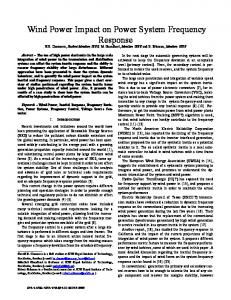
From a good many simulation experiments, the authors find that the transient stability of the power system is very sensitive to the values of X ′′d /X ′d and X ′′q /X ′q . If one of these 2 values is greater than 0.95, under large disturbance, the power angle curve of the generator would oscillate greatly and damp very slowly, and even diverge (i.e. the generator is out of transient stability). Experimental results in Figs. 2 and 3 have illustrated this fact, so the correctness of X ′d, X ′′d, X ′q and X ′′q and their combinations can be tested by transient stability simulation experiments. Fig. 2 shows the power angle curves of GEN3 under 2 different conditions – X d′′ / ′ X d < 0.95, X ′′d /X ′d > 0.95 respectively. The large disturbance set in the experiment is a three-phase permanent fault on 220 kV transmission line BUS1–STATION B: at 0 s a three-phase short-circuit fault occurs on the side of STATION B; at 0.2 s the breakers on both sides trip to clear the fault, but do not reclose. Comparing the curves in Fig. 2 (a) and (b), it can be seen that the former returns to a smooth line quickly, while the latter oscillates ceaselessly and can not damp to a smooth line for a long time. The large disturbance set in Fig. 3’s experiment is the same as that in Fig. 2. Because the power angle curve of GEN3 under condition of X ′′q /X ′q < 0.95 is similar to Fig. 2(a), Fig. 3’s experiment considers only the condition of X ′′q /X ′q > 0.95. But because GEN3 has been out of transient stability under this condition (i.e. out of step with GEN1), the power angle curve deviates too much and has exceeded the drawing ranges of BPA, the power angle curve can not be displayed properly. So the power
Power Angle of GEN3 (°)
Generator Parameters’ Impact on Power System Stability
80 60 40 20 0 −20 3 5 4 6 t/s (a) X d′′ = 0.107 0, X d′ = 0.181 3, X d′′ / X d′ ≈ 0.590 2 < 0.95.
Power Angle of GEN3 (°)
0
1
2
80 60 40 20 0
3 5 4 6 t/s (b) X d′′ = 0.179 0, X d′ = 0.181 3, X d′′ / X d′ ≈ 0.987 3 > 0.95. 0
1
2
Fig. 2. The impact of X ′′d /X ′d on the transient stability of the power system.
System Frequency (Hz)
54 53 52 51 50 49 48 47 46 0
4 6 3 5 t/s X q′′ = 0.22, X q′ = 0.20, X q′′ / X q′ ≈ 1.1 > 0.95. 1
2
Fig. 3. The impact of X ′′q /X ′q on the transient stability of the power system.
265
266
X. Sun et al.
angle curve is replaced by the supervisory curve of the system frequency recorded during the simulation process (shown in Fig. 3), which presents the power system’s status indirectly. From Fig. 3, it can be seen that the system frequency oscillates severely, and already has no chance to return to a smooth line, illustrating the generator is out of transient stability from a different angle. In fact, it is very likely that the transient stability of the power system is not only sensitive to X ′′d /X ′d and X ′′q /X ′q. But the authors merely find these 2 values at present. As to other possible parameter combinations, they still await to be discovered later on. 4.3 Dynamic Stability of Power System
The commonly used procedures for analyzing the dynamic stability of the power system are as follows: 1) Use the small disturbance analysis (the frequency domain method) to calculate each oscillation mode’s real part, imaginary part, frequency, damping ratio and electromechanical circuit correlation ratio, and the modulus and phase angle of the right eigenvector, and the participation factors of the generators participating in the oscillation. 2) Use Prony method (the time domain method) to analyze the active power curves of some important interconnection transmission lines under large disturbance. 3) Try to find out the oscillation modes that are consistent with those found by small disturbance analysis – if the oscillation modes are found, then the results from the frequency domain method are considered to be testified by the time domain method, and accordingly the dynamic stability analysis is considered to be rounded and effective. According to the above procedures, at first, apply the small disturbance analysis to the IEEE 9-node test system. From the small disturbance analysis, 6 oscillation modes are obtained, but only 1 oscillation mode has an electromechanical circuit correlation ratio that is greater than 1, i.e. it is a dominant oscillation mode (DOM). For brevity, the tables and figures in this subsection show only the details of this oscillation mode. Tables 3–7 and Figs. 4–8 have shown the frequency and damping ratio changes of the DOM with GEN3’s parameters T ′d0, T q′ 0, T d′′ 0, T ′′q 0 and TJ respectively (the generator parameters’ changing ranges are determined by Table 1). Table 3 and Fig. 4 show that under small disturbance, with T d′ 0 increasing, the frequency and damping ratio of the DOM are gradually decreasing. Table 4 and Fig. 5 show that under small disturbance, with T ′q 0 increasing, the frequency and damping ratio of the DOM are slightly increasing, but on the whole they are not sensitive to T ′ ′′ q 0. Table 5 and Fig. 6 show that under small disturbance, with T d0 increasing, the frequency of the DOM is basically remaining unchangeable, while the damping ratio is gradually decreasing. Table 6 and Fig. 7 show that under small disturbance, with T ′′ ′′ q 0 increasing, the frequency of the DOM is slightly decreasing (it is not sensitive to T q 0 on the whole), while the damping ratio has a small tendency of increasing. Table 7 and Fig. 8 show that under small disturbance, only when TJ is smaller than a specific value (e.g. smaller than 6.5 s, as shown in the figure), are the frequency and damping ratio of the DOM fairly sensitive to TJ.
Generator Parameters’ Impact on Power System Stability
267
Table 3. The impact of T ′d0 on DOM’s characteristics under small disturbance.
3.00 1.336 4 7.17 7.20 1.295 9 5.44
3.70 1.324 8 6.86 7.90 1.292 9 5.24
4.40 1.315 9 6.53 8.60 1.290 4 5.06
Damping Ratio (%)
Frequency (Hz)
T ′d0 (s) Frequency (Hz) Damping ratio (%) T ′d0 (s) Frequency (Hz) Damping ratio (%)
1.34 1.32 1.30 1.28 3
5
7 9 Td0′ (s) (a) The change of frequency.
5.10 1.309 1 6.21 9.30 1.288 2 4.91
5.80 1.303 8 5.92 10.0 1.286 2 4.76
6.50 1.299 4 5.67
7.0 6.0 5.0 3
5
9 7 Td0′ (s) (b) The change of damping ratio.
Fig. 4. The curves of the impact of T ′d0 on DOM’s characteristics under small disturbance. Table 4. The impact of T ′q0 on DOM’s characteristics under small disturbance.
0.50 1.302 8 5.82 1.40 1.305 7 6.13
0.65 1.303 3 5.92 1.55 1.306 1 6.16
0.80 1.303 9 5.99 1.70 1.306 3 6.17
1.38
Damping Ratio (%)
Frequency (Hz)
T ′q0 (s) Frequency (Hz) Damping ratio (%) T ′q0 (s) Frequency (Hz) Damping ratio (%)
1.34 1.30 1.26 1.22 0.5
1
Tq0′ (s)
1.5
(a) The change of frequency.
2
0.95 1.304 4 6.04 1.85 1.306 7 6.18
1.10 1.304 9 6.08 2.00 1.306 9 6.19
1.25 1.305 5 6.12
1.5
2
6.8 6.4 6.0 5.6 5.2 0.5
1
Tq0′ (s)
(b) The change of damping ratio.
Fig. 5. The curves of the impact of T ′q0 on DOM’s characteristics under small disturbance.
268
X. Sun et al. Table 5. The impact of T ′′d 0 on DOM’s characteristics under small disturbance.
T ′′d 0 (s) Frequency (Hz) Damping ratio (%) T ′′d 0 (s) Frequency (Hz) Damping ratio (%)
0.020 1.302 3 6.30 0.038 1.303 3 5.74
0.023 1.302 5 6.20 0.041 1.303 4 5.65
Damping Ratio (%)
Frequency (Hz)
1.38
0.026 1.302 8 6.10 0.044 1.303 4 5.57
1.34 1.30 1.26 1.22 0.02
0.03 0.04 Td0′′ (s)
0.029 1.303 0 6.01 0.047 1.303 4 5.49
0.032 1.303 2 5.89 0.050 1.303 3 5.41
0.035 1.303 2 5.83
6.3 6.1 5.9 5.7 5.5 0.02
0.05
(a) The change of frequency.
0.03 0.04 Td0′′ (s)
0.05
(b) The change of damping ratio.
Fig. 6. The curves of the impact of T ′′d 0 on DOM’s characteristics under small disturbance. Table 6. The impact of T ′′q 0 on DOM’s characteristics under small disturbance.
0.020 1.308 8 5.53 0.050 1.304 9 5.75
0.025 1.308 0 5.57 0.055 1.304 4 5.79
0.030 1.307 2 5.60 0.060 1.303 9 5.82
Damping Ratio (%)
T ′′q 0 (s) Frequency (Hz) Damping ratio (%) T ′′q 0 (s) Frequency (Hz) Damping ratio (%)
Frequency (Hz)
1.38 1.34 1.30 1.26 1.22
0.035 1.306 6 5.64 0.065 1.303 5 5.85
0.040 1.306 0 5.68 0.070 1.303 2 5.89
0.045 1.305 4 5.71
5.9 5.7 5.5 5.3 5.1
0.02 0.03 0.04 0.05 0.06 0.07 Tq0′′ (s)
0.02 0.03 0.04 0.05 0.06 0.07 Tq0′′ (s)
(a) The change of frequency.
(b) The change of damping ratio.
Fig. 7. The curves of the impact of T ′′q 0 on DOM’s characteristics under small disturbance.
Generator Parameters’ Impact on Power System Stability
269
Table 7. The impact of TJ on DOM’s characteristics under small disturbance.
TJ (s) Frequency (Hz) Damping ratio (%) TJ (s) Frequency (Hz) Damping ratio (%)
4.40 1.301 7 5.70 6.80 1.317 5 6.59
4.80 1.303 7 5.94 7.20 1.320 1 6.61
Damping Ratio (%)
4.00 1.300 1 5.41 6.40 1.314 7 6.53
Frequency (Hz)
1.38 1.34 1.30 1.26 1.22 4
5
6 TJ (s)
7
(a) The change of frequency.
8
5.20 1.306 2 6.15 7.60 1.322 6 6.61
5.60 1.308 9 6.32 8.00 1.324 8 6.60
6.00 1.311 8 6.45
7.0 6.6 6.2 5.8 5.4 4
5
7 6 8 TJ (s) (b) The change of damping ratio.
Fig. 8. The curves of the impact of TJ on DOM’s characteristics under small disturbance.
Next, use the time domain method (under large disturbance) to testify the experimental results obtained from small disturbance analysis. The large disturbance set in the experiment is the same three-phase permanent fault on 220 kV transmission line BUS1–STATION B as mentioned in Subsection 4.2. And the active power curve of the 220 kV transmission line BUS2–STATION A is analyzed by Prony method. Likewise, Tables 8–12 and Figs. 9–13 have shown the frequency and damping ratio changes of the DOM with GEN3’s parameters T d′ 0, T q′ 0, T ′′d 0, T ′′q 0 and TJ respectively under this condition. Table 8 and Fig. 9 show that under large disturbance, with T ′d 0 increasing, the frequency of the DOM is gradually decreasing, while the damping ratio is firstly increasing and then (to about 6 s) decreasing. Table 9 and Fig. 10 show that under large disturbance, with T q′ 0 increasing, the frequency and damping ratio of the DOM are slightly oscillating across a straight line and their mean values are basically remaining unchangeable. Table 10 and Fig. 11 show that under large disturbance, with T ′′d0 increasing, the frequency of the DOM is not sensitive to T d′′0 and is basically remaining unchangeable, while the damping ratio is firstly increasing and then (to about 0.035 s) decreasing. Table 11 and Fig. 12 show that under large disturbance, with T q′′ 0 increasing, the frequency of the DOM is slightly decreasing, while the damping ratio has a tendency of increasing. Table 12 and Fig. 13 show that under large disturbance, only when TJ is smaller than a specific value (e.g. smaller than 6.5 s, as shown in the figure) is the frequency of the DOM fairly sensitive to TJ, while the damping ratio is firstly increasing and then (to about 4.7 s) decreasing.
270
X. Sun et al. Table 8. The impact of T ′d0 on DOM’s characteristics under large disturbance.
3.00 1.366 14.100 7.20 1.142 15.039
3.70 1.341 16.299 7.90 1.137 13.519
4.40 1.309 18.870 8.60 1.133 12.315
Damping Ratio (%)
Frequency (Hz)
T ′d0 (s) Frequency (Hz) Damping ratio (%) T ′d0 (s) Frequency (Hz) Damping ratio (%)
1.4 1.3 1.2 1.1 3
5
7 9 Td0′ (s) (a) The change of frequency.
5.10 1.241 20.834 9.30 1.130 11.375
5.80 1.245 28.129 10.0 1.127 10.545
6.50 1.152 17.284
28 24 20 16 12 3
5
9 7 Td0′ (s) (b) The change of damping ratio.
Fig. 9. The curves of the impact of T ′d0 on DOM’s characteristics under large disturbance. Table 9. The impact of T ′q0 on DOM’s characteristics under large disturbance.
0.50 1.162 19.826 1.40 1.137 23.974
0.65 1.153 20.667 1.55 1.188 21.453
0.80 1.160 21.922 1.70 1.187 21.711
Damping Ratio (%)
Frequency (Hz)
T ′q0 (s) Frequency (Hz) Damping ratio (%) T ′q0 (s) Frequency (Hz) Damping ratio (%)
1.35 1.25 1.15 1.05 0.5
1
1.5 Tq0′ (s)
2
(a) The of change frequency.
0.95 1.212 20.643 1.85 1.200 20.818
1.10 1.137 23.690 2.00 1.124 24.803
1.25 1.174 20.886
28 26 24 22 20 18 0.5
1
Tq0′ (s)
1.5
2
(b) The change of damping ratio.
Fig. 10. The curves of the impact of T ′q0 on DOM’s characteristics under large disturbance.
Generator Parameters’ Impact on Power System Stability
271
Table 10. The impact of T ′′d 0 on DOM’s characteristics under large disturbance.
T ′′d 0 (s) Frequency (Hz) Damping ratio (%) T ′′d 0 (s) Frequency (Hz) Damping ratio (%)
0.020 1.262 25.667 0.038 1.194 31.080
0.023 1.203 24.390 0.041 1.184 18.083
Damping Ratio (%)
Frequency (Hz)
1.45
0.026 1.251 26.483 0.044 1.186 17.250
1.35 1.25 1.15 1.05 0.02
0.03 0.04 Td0′′ (s)
(a) The change of frequency.
0.032 1.219 28.185 0.050 1.192 16.095
0.035 1.174 30.647
30 26 22 18 0.02
0.05
0.029 1.166 22.538 0.047 1.189 16.728
0.03 0.04 Td0′′ (s)
0.05
(b) The change of damping ratio.
Fig. 11. The curves of the impact of T ′′d 0 on DOM’s characteristics under large disturbance. Table 11. The impact of T ′′q 0 on DOM’s characteristics under large disturbance.
0.020 1.198 17.260 0.050 1.180 17.896
0.025 1.195 17.330 0.055 1.175 19.287
1.25 1.20 1.15 1.10 1.05 1.00 0.02 0.03 0.04 0.05 0.06 0.07 Tq0′′ (s) (a) The change of frequency.
0.030 1.190 17.199 0.060 1.172 20.799
Damping Ratio (%)
Frequency (Hz)
T ′′q 0 (s) Frequency (Hz) Damping ratio (%) T ′′q 0 (s) Frequency (Hz) Damping ratio (%)
0.035 1.191 17.756 0.065 1.166 21.297
0.040 1.182 18.688 0.070 1.186 29.204
0.045 1.173 18.955
28 26 24 22 20 18 16 0.02 0.03 0.04 0.05 0.06 0.07 Tq0′′ (s) (b) The change of damping ratio.
Fig. 12. The curves of the impact of T ′′q 0 on DOM’s characteristics under large disturbance.
272
X. Sun et al. Table 12. The impact of TJ on DOM’s characteristics under large disturbance.
4.00 1.144 14.950 6.40 1.285 17.844
4.40 1.149 17.870 6.80 1.295 17.029
Frequency (Hz)
1.35 1.25 1.15 1.05 4
4.80 1.153 21.542 7.20 1.302 16.399
Damping Ratio (%)
TJ (s) Frequency (Hz) Damping ratio (%) TJ (s) Frequency (Hz) Damping ratio (%)
5
6 7 8 TJ (s) (a) The change of frequency.
5.20 1.205 21.070 7.60 1.309 15.782
5.60 1.249 19.780 8.00 1.310 15.445
6.00 1.268 18.923
21 19 17 15 4
5
6
TJ (s)
7
8
(b) The change of damping ratio.
Fig. 13. The curves of the impact of TJ on DOM’s characteristics under large disturbance.
Now, comparing the experimental results obtained from the time domain method (under large disturbance) with those obtained from the frequency domain method (under small disturbance) one by one, the following facts can be seen: as to the frequency changes of the DOM with the generator parameters, the conclusions from both the time domain analysis and the frequency domain analysis are consistent with each other; while as to the damping ratio changes of the DOM with the generator parameters, except for T q′ 0 and T ′′q 0, the conclusions from the time domain analysis and the frequency domain analysis are all different. The reasons for this can be explained as follows: on one hand, the frequency of an oscillation mode is actually the characteristic frequency of the power system that is determined by the inherent structural characters of the power system and is irrelevant to the operation mode and the type of the disturbance, so the conclusions related to frequencies must conform both under small disturbance and under large disturbance; on the other hand, the damping ratio is not an inherent character of the power system, so it would be affected by the operation mode, the parameters and the disturbance types of the power system, and this leads to the differences of the conclusions under small disturbance and under large disturbance. Finally, 3 points should be pointed out. 1) As to the non-dominant oscillation mode, the rules of its frequency and damping ratio changing with the generator parameters are similar to those of the DOM, so the conclusions obtained from the DOM are applicable to the non-dominant oscillation mode. 2) When the experimental results (rules) in this subsection are used to test the generator parameters, some parameters’ impacts on the frequency and damping ratio of the oscillation mode are
Generator Parameters’ Impact on Power System Stability
273
too small to be used to test the parameters. 3) When the damping ratio of the oscillation mode is used to test the generator parameters, the results obtained under small disturbance and under large disturbance should be analyzed separately.
5 Test of Excitation System Parameters and PSS Parameters The adjustment of the excitation system and PSS plays a very important role in guaranteeing the stable operations of the generator and the power system, so the parameters of the excitation system and PSS are always considered together with the generator parameters, and are sometimes treated as a component part of the generator parameters. This section is dedicated to proposing 2 engineering methods for testing excitation system parameters and PSS parameters. 5.1 Excitation System Parameters Test
This subsection proposes a method for testing the excitation system parameters, which can be fell into 4 steps: 1) stop the operation of the tested generator’s PSS; 2) separate the tested generator from the electric network; 3) adjust the reference voltage of the excitation system according to a specific function, e.g. step function or ramp function; 4) investigate whether the output voltage of the generator is able to track the reference voltage effectively – the rising edge is steep, the overshoot is small and the steady area is of no great oscillations. A good way to accomplish step 4) is to compare the output voltage curve of the generator obtained from simulation experiment with another classic curve (obtained from the same simulation experiment of a generator which has correct excitation system parameters). If the differences of the 2 curves are fairly small, then the excitation system parameters can be primarily considered to be correct and effective; otherwise, the excitation system parameters would be unreasonable or ineffective, and further measures must be taken to find the mistakes or the parameters must be remeasured from field test. Fig. 14 shows the simulation curves of the excitation system of GEN3 in IEEE 9node test system. For comparison, a classic curve is superposed on the figure. From Fig. 14 (a) and (b), it can be seen that the differences between the experimental curves and the classic curves in both figures are fairly small, implying that under these 2 conditions the excitation system parameters are both correct and effective. The discrepancies between Fig. 14 (a) and (b) lie on the dynamic amplification coefficients of the automatic voltage regulators (AVR) [8] of the excitation system: the former’s dynamic amplification coefficient is big, so the response of the output voltage of the generator is fast but the overshoot is relatively large; the latter’s dynamic amplification coefficient is small, and the output voltage of the generator has no overshoot, but the response of the output voltage is very slow. Because the types of the curves, when the excitation system parameters are incorrect, are numerous but are easy to distinguish, so the curve samples are omitted for brevity.
X. Sun et al.
The Output Voltage of the Generator (p.u.)
274
1.06
The output voltage of GEN3
1.05 1.04
Classic curve
1.03 1.02 1.01 1.00
6 10 8 t/s (a) The dynamic amplification coefficient of the AVR is big.
The Output Voltage of the Generator (p.u.)
0
2
4
Classic curve
1.05 1.04
The output voltage of GEN3
1.03 1.02 1.01 1.00 0
8 6 10 t/s (b) The dynamic amplification coefficient of the AVR is small. 2
4
Fig. 14. The simulation testing of the excitation system.
5.2 PSS Parameters Test
In this subsection, the proposed method for testing the PSS parameters can also be fell into 4 steps: 1) set up the “double machines and double lines” simulation system as shown in Fig. 15(a) (all the parameters of GEN3 are the same as those in IEEE 9-node test system and the parameters of the other components are labeled in the figure); 2) set a three-phase permanent fault on the high-voltage bus of the transformer on one of the two transmission lines – at 0 s a three-phase short-circuit fault occurs, then at 0.1 s the breakers on both sides trip to clear the fault, but do not reclose; 3) switch on and off the PSS of GEN3 respectively; 4) compare the damping speed of the oscillation of GEN3’s output power under these 2 conditions – if the damping speed of the oscillation of the output power is much faster when PSS is switched on than that when PSS is switched off, the PSS
Generator Parameters’ Impact on Power System Stability
275
parameters are considered to be correct and effective; otherwise, the PSS parameters would be incorrect or ineffective, and need to be remeasured by field test. Fig. 15(b) shows the output power curves of GEN3 when PSS is switched on and switched off. From comparison, it can be inferred that the PSS parameters of GEN3 in IEEE 9-node test system are quite correct and effective, considering that when PSS is switched on the output power curve damps to a straight line much faster. Likewise, the curves when the PSS parameters are incorrect are omitted. GEN3
220 kV I,II:Z = 0.052 78 + j0.079 94 p.u. B/2 = j0.004 74 p.u.
13.8 kV
X d′ = 0
Transformation ratio=13.8:220 Leakage reactance=0.062 5 p.u.
L: 195 + j100 (MW, Mvar) (a) Double machines and double lines simulation system.
TJ = ∞
:
G 0 + j0
The Output Power of GEN3 (MW)
25 20
PSS is switched off
15 10 50 PSS is switched on
0
−50
6 10 8 t/s (b) The output power curve of the generator. 0
2
4
Fig. 15. The simulation testing of the PSS.
6 Conclusion This paper summarizes the impact of the generator parameters (including the parameters of the generator model, excitation system and PSS) on power system’s transient and dynamic stabilities from a good many simulation experiments. Since the experimenting process is closely related to the engineering practice and does not involve any complex theoretical analysis, the summarized rules and conclusions are very evident and practical, and can be directly referenced or applied by the technicians. Based on the rules and conclusions some feasible methods are proposed for testing the generator parameters quickly, which may greatly promote the working
276
X. Sun et al.
efficiencies of the technicians. Although the computational example used in this paper is very simple, the resultant conclusions are of generalization and can be easily testified by readers in their researching and working activities.
References 1. Aghamohammadi, M.R., Beik Khormizi, A., Rezaee, M.: Effect of Generator Parameters Inaccuracy on Transient Stability Performance. In: IEEE Asia-Pacific Power and Energy Engineering Conference (APPEEC), pp. 1–5 (2010) 2. Shouzhen, Z., Shande, S., Houlian, C., Jianmin, J.: Effects of the Excitation System Parameters on Power System Transient Stability Studies. In: The 2nd IET International Conference on Advances in Power System Control, Operation and Management, vol. 2, pp. 532–535 (1993) 3. Lidenholm, J., Lundin, U.: Estimation of Hydropower Generator Parameters Through Field Simulations of Standard Tests. IEEE Transactions on Energy Conversion 25, 931–939 (2010) 4. Kundur, P.: Power System Stability and Control. The McGraw-Hill Companies, Inc., New York (1994) 5. IEEE Power Engineering Society: IEEE Guide for Synchronous Generator Modeling Practices and Applications in Power System Stability Analyses. IEEE Std 1110-2002, pp. 1–72 (2003) 6. Wuzhi, Z., Xinli, S., Yong, T., Guangquan, B., Qiang, G.: New Research and Exploitation of Power System Small Signal Stability Analysis Software. In: International Conference on Electrical Engineering (ICEE), pp. 1–5 (2006) 7. PSD Software Program Training Manual, http://wenku.baidu.com/view/552a33e9856a561252d36f08.html 8. Hoong, C.S., Taib, T., Rao, K.S., Daut, I.: Development of Automatic Voltage Regulator for Synchronous Generator. In: Proceedings of Power and Energy Conference (PECon), pp. 180–184 (2004)