Genetic Algorithm and Direct Search Toolbox User's Guide

Genetic Algorithm and Direct Search Toolbox For Use with MATLAB

®

User’s Guide Version 1

How to Contact The MathWorks: www.mathworks.com comp.soft-sys.matlab

Web Newsgroup

[email protected]

Technical support Product enhancement suggestions Bug reports Documentation error reports Order status, license renewals, passcodes Sales, pricing, and general information

508-647-7000

Phone

508-647-7001

Fax

The MathWorks, Inc. 3 Apple Hill Drive Natick, MA 01760-2098

Mail

[email protected] [email protected] [email protected] [email protected] [email protected]

For contact information about worldwide offices, see the MathWorks Web site. Genetic Algorithm and Direct Search Toolbox User’s Guide  COPYRIGHT 2004 by The MathWorks, Inc. The software described in this document is furnished under a license agreement. The software may be used or copied only under the terms of the license agreement. No part of this manual may be photocopied or reproduced in any form without prior written consent from The MathWorks, Inc. FEDERAL ACQUISITION: This provision applies to all acquisitions of the Program and Documentation by or for the federal government of the United States. By accepting delivery of the Program, the government hereby agrees that this software qualifies as "commercial" computer software within the meaning of FAR Part 12.212, DFARS Part 227.7202-1, DFARS Part 227.7202-3, DFARS Part 252.227-7013, and DFARS Part 252.227-7014. The terms and conditions of The MathWorks, Inc. Software License Agreement shall pertain to the government’s use and disclosure of the Program and Documentation, and shall supersede any conflicting contractual terms or conditions. If this license fails to meet the government’s minimum needs or is inconsistent in any respect with federal procurement law, the government agrees to return the Program and Documentation, unused, to MathWorks. MATLAB, Simulink, Stateflow, Handle Graphics, and Real-Time Workshop are registered trademarks, and TargetBox is a trademark of The MathWorks, Inc. Other product or brand names are trademarks or registered trademarks of their respective holders.

Printing History: January 2004

Online only

New for Version 1.0 (Release 13SP1+)

Contents Introducing the Genetic Algorithm and Direct Search Toolbox

1 What Is the Genetic Algorithm and Direct Search Toolbox? . . . . . . . . . . . . . . . . . . . . . . . . . . . . . . . . . . . . . . . . . . . . . 1-2 Related Products . . . . . . . . . . . . . . . . . . . . . . . . . . . . . . . . . . . . . 1-3 Writing an M-File for the Function You Want to Optimize 1-5 Example — Writing an M-File . . . . . . . . . . . . . . . . . . . . . . . . . . 1-5 Maximizing Versus Minimizing . . . . . . . . . . . . . . . . . . . . . . . . . 1-6

Getting Started with the Genetic Algorithm

2 What Is the Genetic Algorithm? . . . . . . . . . . . . . . . . . . . . . . . . 2-2 Using The Genetic Algorithm . . . . . . . . . . . . . . . . . . . . . . . . . . 2-3 Calling the Function ga at the Command Line . . . . . . . . . . . . . 2-3 Using the Genetic Algorithm Tool . . . . . . . . . . . . . . . . . . . . . . . 2-4 Example: Rastrigin’s Function . . . . . . . . . . . . . . . . . . . . . . . . . 2-6 Rastrigin’s Function . . . . . . . . . . . . . . . . . . . . . . . . . . . . . . . . . . 2-6 Finding the Minimum of Rastrigin’s Function . . . . . . . . . . . . . 2-8 Finding the Minimum from the Command Line . . . . . . . . . . . 2-10 Displaying Plots . . . . . . . . . . . . . . . . . . . . . . . . . . . . . . . . . . . . . 2-11 Some Genetic Algorithm Terminology . . . . . . . . . . . . . . . . . Fitness Functions . . . . . . . . . . . . . . . . . . . . . . . . . . . . . . . . . . . Individuals . . . . . . . . . . . . . . . . . . . . . . . . . . . . . . . . . . . . . . . . . Populations and Generations . . . . . . . . . . . . . . . . . . . . . . . . . . Diversity . . . . . . . . . . . . . . . . . . . . . . . . . . . . . . . . . . . . . . . . . . . Fitness Values and Best Fitness Values . . . . . . . . . . . . . . . . . Parents and Children . . . . . . . . . . . . . . . . . . . . . . . . . . . . . . . .

2-15 2-15 2-15 2-15 2-16 2-16 2-17

iii

How the Genetic Algorithm Works . . . . . . . . . . . . . . . . . . . . . Outline of the Algorithm . . . . . . . . . . . . . . . . . . . . . . . . . . . . . . Initial Population . . . . . . . . . . . . . . . . . . . . . . . . . . . . . . . . . . . . Creating the Next Generation . . . . . . . . . . . . . . . . . . . . . . . . . . Plots of Later Generations . . . . . . . . . . . . . . . . . . . . . . . . . . . . . Stopping Conditions for the Algorithm . . . . . . . . . . . . . . . . . . .

2-18 2-18 2-19 2-20 2-23 2-24

Getting Started with Direct Search

3 What Is Direct Search? . . . . . . . . . . . . . . . . . . . . . . . . . . . . . . . . 3-2 Performing a Pattern Search . . . . . . . . . . . . . . . . . . . . . . . . . . . 3-3 Calling patternsearch at the Command Line . . . . . . . . . . . . . . . 3-3 Using the Pattern Search Tool . . . . . . . . . . . . . . . . . . . . . . . . . . 3-3

iv

Contents

Example: Finding the Minimum of a Function . . . . . . . . . . . Objective Function . . . . . . . . . . . . . . . . . . . . . . . . . . . . . . . . . . . . Finding the Minimum of the Function . . . . . . . . . . . . . . . . . . . . Plotting the Objective Function Values and Mesh Sizes . . . . . .

3-6 3-6 3-7 3-8

Pattern Search Terminology . . . . . . . . . . . . . . . . . . . . . . . . . . Patterns . . . . . . . . . . . . . . . . . . . . . . . . . . . . . . . . . . . . . . . . . . . Meshes . . . . . . . . . . . . . . . . . . . . . . . . . . . . . . . . . . . . . . . . . . . . Polling . . . . . . . . . . . . . . . . . . . . . . . . . . . . . . . . . . . . . . . . . . . . .

3-10 3-10 3-11 3-12

How Pattern Search Works . . . . . . . . . . . . . . . . . . . . . . . . . . . Iterations 1 and 2: Successful Polls . . . . . . . . . . . . . . . . . . . . . Iteration 4: An Unsuccessful Poll . . . . . . . . . . . . . . . . . . . . . . . Displaying the Results at Each Iteration . . . . . . . . . . . . . . . . . More Iterations . . . . . . . . . . . . . . . . . . . . . . . . . . . . . . . . . . . . . . Stopping Conditions for the Pattern Search . . . . . . . . . . . . . . .

3-13 3-13 3-16 3-17 3-17 3-18

Using the Genetic Algorithm

4 Overview of the Genetic Algorithm Tool . . . . . . . . . . . . . . . . 4-2 Opening the Genetic Algorithm Tool . . . . . . . . . . . . . . . . . . . . . 4-2 Defining a Problem in the Genetic Algorithm Tool . . . . . . . . . . 4-3 Running the Genetic Algorithm . . . . . . . . . . . . . . . . . . . . . . . . . 4-4 Pausing and Stopping the Algorithm . . . . . . . . . . . . . . . . . . . . . 4-5 Displaying Plots . . . . . . . . . . . . . . . . . . . . . . . . . . . . . . . . . . . . . . 4-7 Example — Creating a Custom Plot Function . . . . . . . . . . . . . . 4-8 Reproducing Your Results . . . . . . . . . . . . . . . . . . . . . . . . . . . . . 4-11 Setting Options for the Genetic Algorithm . . . . . . . . . . . . . . . . 4-11 Importing and Exporting Options and Problems . . . . . . . . . . . 4-13 Example — Resuming the Genetic Algorithm from the Final Population: . . . . . . . . . . . . . . . . . . . . . . . . . . . . . . . . . . . . 4-16 Generating an M-File . . . . . . . . . . . . . . . . . . . . . . . . . . . . . . . . 4-20 Using the Genetic Algorithm from the Command Line . . . Running the Genetic Algorithm with the Default Options . . . Setting Options . . . . . . . . . . . . . . . . . . . . . . . . . . . . . . . . . . . . . Using Options and Problems from the Genetic Algorithm Tool . . . . . . . . . . . . . . . . . . . . . . . . . . . . . . . . . . . . . . . . . . . . . . . Reproducing Your Results . . . . . . . . . . . . . . . . . . . . . . . . . . . . . Resuming ga from the Final Population of a Previous Run . . Running ga from an M-File . . . . . . . . . . . . . . . . . . . . . . . . . . . .

4-21 4-21 4-22

Setting Options for the Genetic Algorithm . . . . . . . . . . . . . Diversity . . . . . . . . . . . . . . . . . . . . . . . . . . . . . . . . . . . . . . . . . . . Population Options . . . . . . . . . . . . . . . . . . . . . . . . . . . . . . . . . . Fitness Scaling Options . . . . . . . . . . . . . . . . . . . . . . . . . . . . . . . Selection Options . . . . . . . . . . . . . . . . . . . . . . . . . . . . . . . . . . . . Reproduction Options . . . . . . . . . . . . . . . . . . . . . . . . . . . . . . . . Mutation and Crossover . . . . . . . . . . . . . . . . . . . . . . . . . . . . . . Mutation Options . . . . . . . . . . . . . . . . . . . . . . . . . . . . . . . . . . . . The Crossover Fraction . . . . . . . . . . . . . . . . . . . . . . . . . . . . . . . Comparing Results for Varying Crossover Fractions . . . . . . . Example — Global Versus Local Minima . . . . . . . . . . . . . . . . . Setting the Maximum Number of Generations . . . . . . . . . . . . Using a Hybrid Function . . . . . . . . . . . . . . . . . . . . . . . . . . . . . . Vectorize Option . . . . . . . . . . . . . . . . . . . . . . . . . . . . . . . . . . . . .

4-29 4-29 4-30 4-34 4-38 4-39 4-39 4-40 4-42 4-45 4-47 4-51 4-53 4-55

4-24 4-25 4-26 4-26

v

Using Direct Search

5 Overview of the Pattern Search Tool . . . . . . . . . . . . . . . . . . . . 5-2 Opening the Pattern Search Tool . . . . . . . . . . . . . . . . . . . . . . . . 5-2 Defining a Problem in the Pattern Search Tool . . . . . . . . . . . . . 5-3 Running a Pattern Search . . . . . . . . . . . . . . . . . . . . . . . . . . . . . . 5-5 Example — A Constrained Problem . . . . . . . . . . . . . . . . . . . . . . 5-6 Pausing and Stopping the Algorithm . . . . . . . . . . . . . . . . . . . . . 5-8 Displaying Plots . . . . . . . . . . . . . . . . . . . . . . . . . . . . . . . . . . . . . . 5-8 Setting Options . . . . . . . . . . . . . . . . . . . . . . . . . . . . . . . . . . . . . . 5-9 Importing and Exporting Options and Problems . . . . . . . . . . . 5-10 Generate M-File . . . . . . . . . . . . . . . . . . . . . . . . . . . . . . . . . . . . . 5-13 Performing a Pattern Search from the Command Line . . Performing a Pattern Search with the Default Options . . . . . Setting Options . . . . . . . . . . . . . . . . . . . . . . . . . . . . . . . . . . . . . Using Options and Problems from the Pattern Search Tool . .

5-14 5-14 5-16 5-18

Setting Pattern Search Options . . . . . . . . . . . . . . . . . . . . . . . Poll Method . . . . . . . . . . . . . . . . . . . . . . . . . . . . . . . . . . . . . . . . Complete Poll . . . . . . . . . . . . . . . . . . . . . . . . . . . . . . . . . . . . . . . Using a Search Method . . . . . . . . . . . . . . . . . . . . . . . . . . . . . . . Mesh Expansion and Contraction . . . . . . . . . . . . . . . . . . . . . . . Mesh Accelerator . . . . . . . . . . . . . . . . . . . . . . . . . . . . . . . . . . . . Cache Options . . . . . . . . . . . . . . . . . . . . . . . . . . . . . . . . . . . . . . Setting Tolerances for the Solver . . . . . . . . . . . . . . . . . . . . . . .

5-19 5-19 5-21 5-25 5-28 5-33 5-35 5-37

Function Reference

6 Functions — Listed by Category . . . . . . . . . . . . . . . . . . . . . . . . 6-2 Genetic Algorithm . . . . . . . . . . . . . . . . . . . . . . . . . . . . . . . . . . . . 6-2 Direct Search . . . . . . . . . . . . . . . . . . . . . . . . . . . . . . . . . . . . . . . . 6-2 Genetic Algorithm Options . . . . . . . . . . . . . . . . . . . . . . . . . . . . . 6-3 Plot Options . . . . . . . . . . . . . . . . . . . . . . . . . . . . . . . . . . . . . . . . . 6-4

vi

Contents

Population Options . . . . . . . . . . . . . . . . . . . . . . . . . . . . . . . . . . . 6-5 Fitness Scaling Options . . . . . . . . . . . . . . . . . . . . . . . . . . . . . . . . 6-7 Selection Options . . . . . . . . . . . . . . . . . . . . . . . . . . . . . . . . . . . . . 6-8 Reproduction Options . . . . . . . . . . . . . . . . . . . . . . . . . . . . . . . . 6-10 Mutation Options . . . . . . . . . . . . . . . . . . . . . . . . . . . . . . . . . . . . 6-10 Crossover Options . . . . . . . . . . . . . . . . . . . . . . . . . . . . . . . . . . . 6-12 Migration Options . . . . . . . . . . . . . . . . . . . . . . . . . . . . . . . . . . . 6-15 Output Function Options . . . . . . . . . . . . . . . . . . . . . . . . . . . . . . 6-16 Stopping Criteria Options . . . . . . . . . . . . . . . . . . . . . . . . . . . . . 6-17 Hybrid Function Option . . . . . . . . . . . . . . . . . . . . . . . . . . . . . . . 6-17 Vectorize Option . . . . . . . . . . . . . . . . . . . . . . . . . . . . . . . . . . . . . 6-17 The State Structure . . . . . . . . . . . . . . . . . . . . . . . . . . . . . . . . . . 6-18 Pattern Search Options . . . . . . . . . . . . . . . . . . . . . . . . . . . . . . . Plot Options . . . . . . . . . . . . . . . . . . . . . . . . . . . . . . . . . . . . . . . . Poll Options . . . . . . . . . . . . . . . . . . . . . . . . . . . . . . . . . . . . . . . . Search Options . . . . . . . . . . . . . . . . . . . . . . . . . . . . . . . . . . . . . . Mesh Options . . . . . . . . . . . . . . . . . . . . . . . . . . . . . . . . . . . . . . . Cache Options . . . . . . . . . . . . . . . . . . . . . . . . . . . . . . . . . . . . . . Stopping Criteria . . . . . . . . . . . . . . . . . . . . . . . . . . . . . . . . . . . . Output Function Options . . . . . . . . . . . . . . . . . . . . . . . . . . . . . . Display to Command Window Options . . . . . . . . . . . . . . . . . . . Vectorize Option . . . . . . . . . . . . . . . . . . . . . . . . . . . . . . . . . . . . .

6-19 6-20 6-20 6-22 6-24 6-25 6-25 6-26 6-26 6-27

Functions — Alphabetical List . . . . . . . . . . . . . . . . . . . . . . . . 6-28

Index

vii

viii Contents

1 Introducing the Genetic Algorithm and Direct Search Toolbox

What Is the Genetic Algorithm and Direct Search Toolbox? (p. 1-2)

Introduces the toolbox and its features.

Related Products (p. 1-3)

Lists products that are relevant to the kinds of tasks you can perform with the Genetic Algorithm and Direct Search Toolbox.

Writing an M-File for the Function You Explains how to solve maximization as well as Want to Optimize (p. 1-5) minimization problems using the toolbox.

1

Introducing the Genetic Algorithm and Direct Search Toolbox

What Is the Genetic Algorithm and Direct Search Toolbox? The Genetic Algorithm and Direct Search Toolbox is a collection of functions that extend the capabilities of the Optimization Toolbox and the MATLAB® numeric computing environment. The Genetic Algorithm and Direct Search Toolbox includes routines for solving optimization problems using • Genetic algorithm • Direct search These algorithms enable you to solve a variety of optimization problems that lie outside the scope of the standard Optimization Toolbox. All the toolbox functions are MATLAB M-files, made up of MATLAB statements that implement specialized optimization algorithms. You can view the MATLAB code for these functions using the statement type function_name

You can extend the capabilities of the Genetic Algorithm and Direct Search Toolbox by writing your own M-files, or by using the toolbox in combination with other toolboxes, or with MATLAB or Simulink®.

1-2

Related Products

Related Products The MathWorks provides several products that are relevant to the kinds of tasks you can perform with the Genetic Algorithm and Direct Search Toolbox. For more information about any of these products, see either • The online documentation for that product, if it is installed or if you are reading the documentation from the CD • The MathWorks Web site, at http://www.mathworks.com; see the “products” section

Note The following toolboxes all include functions that extend the capabilities of MATLAB. The blocksets all include blocks that extend the capabilites of Simulink.

Product

Description

Curve Fitting Toolbox

Perform model fitting and analysis

Data Acquisition Toolbox

Acquire and send out data from plug-in data acquisition boards

Database Toolbox

Exchange data with relational databases

Financial Time Series Toolbox

Analyze and manage financial time-series data

Financial Toolbox

Model financial data and develop financial analysis algorithms

GARCH Toolbox

Analyze financial volatility using univariate GARCH models

LMI Control Toolbox

Design robust controllers using convex optimization techniques

Neural Network Toolbox

Design and simulate neural networks

1-3

1


1-4

Product

Description

Nonlinear Control Design Blockset

Optimize design parameters in nonlinear control systems

Optimization Toolbox

Solve standard and large-scale optimization problems

Signal Processing Toolbox

Perform signal processing, analysis, and algorithm development

Simulink

Design and simulate continuous- and discrete-time systems

Spline Toolbox

Create and manipulate spline approximation models of data

Statistics Toolbox

Apply statistical algorithms and probability models

Symbolic/Extended Symbolic Math Toolbox

Perform computations using symbolic mathematics and variable-precision arithmetic

System Identification Toolbox

Create linear dynamic models from measured input-output data

Writing an M-File for the Function You Want to Optimize

Writing an M-File for the Function You Want to Optimize To use the Genetic Algorithm and Direct Search Toolbox, you must first write an M-file that computes the function you want to optimize. The M-file should accept a row vector, whose length is the number of independent variables for the objective function, and return a scalar. This section explains how to write the M-file and covers the following topics: • “Example — Writing an M-File” on page 1-5 • “Maximizing Versus Minimizing” on page 1-6

Example — Writing an M-File The following example shows how to write an M-file for the function you want to optimize. Suppose that you want to minimize the function 2

2

f (x 1, x 2) = x 1 – 2x 1 x 2 + 6x 1 + x 2 – 6x 2 The M-file that computes this function must accept a row vector x of length 2, corresponding to the variables x1 and x2, and return a scalar equal to the value of the function at x. To write the M-file, do the following steps: 1 Select New in the MATLAB File menu. 2 Select M-File. This opens a new M-file in the editor. 3 In the M-file, enter the following two lines of code:

function z = my_fun(x) z = x(1)^2 - 2*x(1)*x(2) + 6*x(1) + x(2)^2 - 6*x(2); 4 Save the M-file in a directory on the MATLAB path.

To check that the M-file returns the correct value, enter my_fun([2 3]) ans = -5

1-5

1


Note Do not use the Editor/Debugger to debug the M-file for the objective function while running the Genetic Algorithm Tool or the Pattern Search Tool. Doing so results in Java exception messages in the Command Window and makes debugging more difficult. See either “Defining a Problem in the Genetic Algorithm Tool” on page 4-3 or “Defining a Problem in the Pattern Search Tool” on page 5-3 for more information on debugging.

Maximizing Versus Minimizing The optimization functions in the Genetic Algorithm and Direct Search Toolbox minimize the objective or fitness function. That is, they solve problems of the form minimize f ( x ) x If you want to maximize f(x), you can do so by minimizing -f(x), because the point at which the minimum of -f(x) occurs is the same as the point at which the maximum of f(x) occurs. For example, suppose you want to maximize the function 2

2

f (x 1, x 2) = x 1 – 2x 1 x 2 + 6x 1 + x 2 – 6x 2 described in the preceding section. In this case, you should write your M-file to compute 2

2

– f (x 1, x 2) = – x 1 + 2x 1 x 2 – 6x 1 – x 2 + 6x 2 and minimize this function.

1-6

2 Getting Started with the Genetic Algorithm

What Is the Genetic Algorithm? (p. 2-2) Introduces the genetic algorithm. Using The Genetic Algorithm (p. 2-3)

Explains how to use the genetic algorithm tool.

Example: Rastrigin’s Function (p. 2-6)

Presents an example of solving an optimization problem using the genetic algorithm.

Some Genetic Algorithm Terminology (p. 2-15)

Explains some basic terminology for the genetic algorithm.

How the Genetic Algorithm Works (p. 2-18)

Presents an overview of how the genetic algorithm works.

2


What Is the Genetic Algorithm? The genetic algorithm is a method for solving optimization problems that is based on natural selection, the process that drives biological evolution. The genetic algorithm repeatedly modifies a population of individual solutions. At each step, the genetic algorithm selects individuals at random from the current population to be parents and uses them produce the children for the next generation. Over successive generations, the population “evolves” toward an optimal solution. You can apply the genetic algorithm to solve a variety of optimization problems that are not wellsuited for standard optimization algorithms, including problems in which the objective function is discontinuous, nondifferentiable, stochastic, or highly nonlinear. The genetic algorithm uses three main types of rules at each step to create the next generation from the current population: • Selection rules select the individuals, called parents, that contribute to the population at the next generation. • Crossover rules combine two parents to form children for the next generation. • Mutation rules apply random changes to individual parents to form children. The genetic algorithm differs from a standard optimization algorithm in two main ways, as summarized in the following table.

2-2

Standard Algorithm

Genetic Algorithm

Generates a single point at each iteration. The sequence of points approaches an optimal solution.

Generates a population of points at each iteration. The population approaches an optimal solution.

Selects the next point in the sequence by a deterministic computation.

Selects the next population by computations that involve random choices.

Using The Genetic Algorithm

Using The Genetic Algorithm There are two ways you can use the genetic algorithm with the toolbox: • Calling the genetic algorithm function ga at the command line. • Using the Genetic Algorithm Tool, a graphical interface to the genetic algorithm. This section provides a brief introduction to these methods.

Calling the Function ga at the Command Line To use the genetic algorithm at the command line, call the genetic algorithm function ga with the syntax [x fval] = ga(@fitnessfun, nvars, options)

where • @fitnessfun is a handle to the fitness function. • nvars is the number of independent variables for the fitness function. • options is a structure containing options for the genetic algorithm. If you do not pass in this argument, ga uses its default options. The results are given by • fval — Final value of the fitness function • x — Point at which the final value is attained Using the function ga is convenient if you want to • Return results directly to the MATLAB workspace • Run the genetic algorithm multiple times with different options, by calling ga from an M-file “Using the Genetic Algorithm from the Command Line” on page 4-21 provides a detailed description of using the function ga and creating the options structure.

2-3

2


Using the Genetic Algorithm Tool The Genetic Algorithm Tool is a graphical user interface that enables you to use the genetic algorithm without working at the command line. To open the Genetic Algorithm Tool, enter gatool

This opens the tool as shown in the following figure. Click to display descriptions of options.

Enter fitness function. Enter number of variables for the fitness function.

Start the genetic algorithm.

Results are displayed here.

2-4

Using The Genetic Algorithm

To use the Genetic Algorithm Tool, you must first enter the following information: • Fitness function — The objective function you want to minimize. Enter the fitness function in the form @fitnessfun, where fitnessfun.m is an M-file that computes the fitness function. “Writing an M-File for the Function You Want to Optimize” on page 1-5 explains how write this M-file. The @ sign creates a function handle to fitnessfun. • Number of variables — The length of the input vector to the fitness function. For the function my_fun described in “Writing an M-File for the Function You Want to Optimize” on page 1-5, you would enter 2. To run the genetic algorithm, click the Start button. The tool displays the results of the optimization in the Status and Results pane. You can change the options for the genetic algorithm in the Options pane. To view the options in one of the categories listed in the pane, click the + sign next to it. For more information, • See “Overview of the Genetic Algorithm Tool” on page 4-2 for a detailed description of the tool. • See “Example: Rastrigin’s Function” on page 2-6 for an example of using the tool.

2-5

2


Example: Rastrigin’s Function This section presents an example that shows how to find the minimum of Rastrigin’s function, a function that is often used to test the genetic algorithm. This section covers the following topics: • “Rastrigin’s Function” on page 2-6 • “Finding the Minimum of Rastrigin’s Function” on page 2-8 • “Displaying Plots” on page 2-11

Rastrigin’s Function For two independent variables, Rastrigin’s function is defined as 2

2

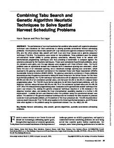
Ras(x) = 20 + x 1 + x 2 – 10 ( cos 2πx 1 + cos 2πx 2 ) The toolbox contains an M-file, rastriginsfcn.m, that computes the values of Rastriginsfcn. The following figure shows a plot of Rastrigin’s function.

2-6

Example: Rastrigin’s Function

Global minimum at [0 0]

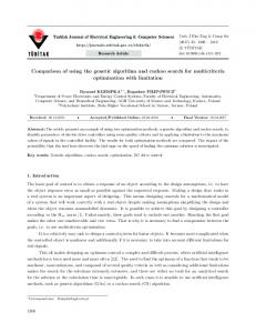
As the plot shows, Rastrigin’s function has many local minima — the “valleys” in the plot. However, the function has just one global minimum, which occurs at the point [0 0] in the x-y plane, as indicated by the vertical line in the plot, where the value of the function is 0. At any local minimum other than [0 0], the value of Rastrigin’s function is greater than 0. The farther the local minimum is from the origin, the larger the value of the function is at that point. Rastrigin’s function is often used to test the genetic algorithm, because its many local minima make it difficult for standard, gradient-based methods to find the global minimum. The following contour plot of Rastrigin’s function shows the alternating maxima and minima.

2-7

2


1 0.8 0.6 0.4

Local maxima

0.2 0 −0.2 −0.4

Local minima

−0.6 −0.8 −1 −1

−0.5

0

0.5

1

Global minimum at [0 0]

Finding the Minimum of Rastrigin’s Function This section explains how to find the minimum of Rastrigin’s function using the genetic algorithm.

Note Because the genetic algorithm uses random data to perform its search, the algorithm returns slightly different results each time you run it.

To find the minimum, do the following steps: 1 Enter gatool at the command line to open the Genetic Algorithm Tool. 2 Enter the following in the Genetic Algorithm Tool:

- In the Fitness function field, enter @rastriginsfcn. - In the Number of variables field, enter 2, the number of independent variables for Rastrigin’s function.

2-8


The Fitness function and Number of variables fields should appear as shown in the following figure.

3 Click the Start button in the Run solver pane, as shown in the following

figure.

Click the Start button

While the algorithm is running, the Current generation field displays the number of the current generation. You can temporarily pause the algorithm by clicking the Pause button. When you do so, the button name changes to Resume. To resume the algorithm from the point at which you paused it, click Resume. When the algorithm is finished, the Status and results pane appears as shown in the following figure.

Fitness function value at final point

Final point

The Status and results pane displays the following information:

2-9

2


• The final value of the fitness function when the algorithm terminated: Function value: 0.0067749206244585025

Note that the value shown is very close to the actual minimum value of Rastrigin’s function, which is 0. “Setting Options for the Genetic Algorithm” on page 4-29 describes some ways to get a result that is closer to the actual minimum. • The reason the algorithm terminated. Exit: Optimization terminated: maximum number of generations exceeded.

In this example, the algorithm terminates after 100 generations, the default value of the option Generations, which specifies the maximum number of generations the algorithm computes. • The final point, which in this example is [0.00274 -0.00516].

Finding the Minimum from the Command Line To find the minimum of Rastrigin’s function from the command line, enter [x fval reason] = ga(@rastriginsfcn, 2)

This returns [x fval reason] = ga(@rastriginsfcn, 2) x = 0.0027

-0.0052

fval = 0.0068

reason = Optimization terminated: maximum number of generations exceeded.

2-10


where • x is the final point returned by the algorithm. • fval is the fitness function value at the final point. • reason is the reason that the algorithm terminated.

Displaying Plots The Plots pane enables you to display various plots that provide information about the genetic algorithm while it is running. This information can help you change options to improve the performance of the algorithm. For example, to plot the best and mean values of the fitness function at each generation, select the box next to Best fitness value, as shown in the following figure.

Select Best fitness

When you click Start, the Genetic Algorithm Tool displays a plot of the best and mean values of the fitness function at each generation. When the algorithm stops, the plot appears as shown in the following figure.

2-11

2


Best: 0.0067796 Mean: 0.014788 18 16 14 12 10 8 6 4 2 0

10

20

30

40

50 60 generation

70

80

90

100

The points at the bottom of the plot denote the best fitness values, while the points above them denote the averages of the fitness values in each generation. The plot also displays the best and mean values in the current generation numerically at the top. To get a better picture of how much the best fitness values are decreasing, you can change the scaling of the y-axis in the plot to logarithmic scaling. To do so, 1 Select Axes Properties from the Edit menu in the plot window to open the

Property Editor, as shown in the following figure.

2-12


Click the Y tab.

Select Log.

2 Click the Y tab. 3 In the Scale pane, select Log.

The plot now appears as shown in the following figure.

2-13

2


Best: 0.0067796 Mean: 0.014788

2

10

1

10

0

10

−1

10

−2

10

−3

10

10

20

30

40

50 60 generation

70

80

90

100

Typically, the best fitness value improves rapidly in the early generations, when the individuals are farther from the optimum. The best fitness value improves more slowly in later generations, whose populations are closer to the optimal point.

2-14

Some Genetic Algorithm Terminology

Some Genetic Algorithm Terminology This section explains some basic terminology for the genetic algorithm, including • “Fitness Functions” on page 2-15 • “Individuals” on page 2-15 • “Populations and Generations” on page 2-15 • “Fitness Values and Best Fitness Values” on page 2-16 • “Parents and Children” on page 2-17

Fitness Functions The fitness function is the function you want to optimize. For standard optimization algorithms, this is known as the objective function. The toolbox tries to find the minimum of the fitness function. You can write the fitness function as an M-file and pass it as an input argument to the main genetic algorithm function.

Individuals An individual is any point to which you can apply the fitness function. The value of the fitness function for an individual is its score. For example, if the fitness function is 2

2

f(x 1, x 2 , x 3) = ( 2x 1 + 1 ) + ( 3x 2 + 4 ) + ( x 3 – 2 )

2

the vector (2, 3, 1), whose length is the number of variables in the problem, is an individual. The score of the individual (2, 3, 1) is f(2, -3, 1) = 51. An individual is sometimes referred to as a genome and the vector entries of an individual as genes.

Populations and Generations A population is an array of individuals. For example, if the size of the population is 100 and the number of variables in the fitness function is 3, you represent the population by a 100-by-3 matrix. The same individual can appear

2-15

2


more than once in the population. For example, the individual (2, 3, 1) can appear in more than one row of the array. At each iteration, the genetic algorithm performs a series of computations on the current population to produce a new population. Each successive population is called a new generation.

Diversity Diversity refers to the average distance between individuals in a population. A population has high diversity if the average distance is large; otherwise it has low diversity. In the following figure, the population on the left has high diversity, while the population on the right has low diversity.

5 High diversity Low diversity

4 3 2 1 0

0

2

4

6

8

Diversity is essential to the genetic algorithm because it enables the algorithm to search a larger region of the space.

Fitness Values and Best Fitness Values The fitness value of an individual is the value of the fitness function for that individual. Because the toolbox finds the minimum of the fitness function, the

2-16

Some Genetic Algorithm Terminology

best fitness value for a population is the smallest fitness value for any individual in the population.

Parents and Children To create the next generation, the genetic algorithm selects certain individuals in the current population, called parents, and uses them to create individuals in the next generation, called children. Typically, the algorithm is more likely to select parents that have better fitness values.

2-17

2


How the Genetic Algorithm Works This section provides an overview of how the genetic algorithm works. This section covers the following topics: • “Outline of the Algorithm” on page 2-18 • “Initial Population” on page 2-19 • “Creating the Next Generation” on page 2-20 • “Plots of Later Generations” on page 2-23 • “Stopping Conditions for the Algorithm” on page 2-24

Outline of the Algorithm The following outline summarizes how the genetic algorithm works: 1 The algorithm begins by creating a random initial population. 2 The algorithm then creates a sequence of new populations, or generations.

At each step, the algorithm uses the individuals in the current generation to create the next generation. To create the new generation, the algorithm performs the following steps: a Scores each member of the current population by computing its fitness

value. b Scales the raw fitness scores to convert them into a more usable range of

values. c

Selects parents based on their fitness.

d Produces children from the parents. Children are produced either by

making random changes to a single parent — mutation — or by combining the vector entries of a pair of parents — crossover. e

Replaces the current population with the children to form the next generation.

3 The algorithm stops when one of the stopping criteria is met. See “Stopping

Conditions for the Algorithm” on page 2-24.

2-18

How the Genetic Algorithm Works

Initial Population The algorithm begins by creating a random initial population, as shown in the following figure.

1 Initial population 0.8 0.6 0.4 0.2 0 −0.2 −0.4 −0.6 −0.8 −1 −1

−0.5

0

0.5

1

In this example, the initial population contains 20 individuals, which is the default value of Population size in the Population options. Note that all the individuals in the initial population lie in the upper-right quadrant of the picture, that is, their coordinates lie between 0 and 1, because the default value of Initial range in the Population options is [0;1]. If you know approximately where the minimal point for a function lies, you should set Initial range so that the point lies near the middle of that range. For example, if you believe that the minimal point for Rastrigin’s function is near the point [0 0], you could set Initial range to be [-1;1]. However, as this example shows, the genetic algorithm can find the minimum even with a less than optimal choice for Initial range.

2-19

2


Creating the Next Generation At each step, the genetic algorithm uses the current population to create the children that make up the next generation. The algorithm selects a group of individuals in the current population, called parents, who contribute their genes — the entries of their vectors — to their children. The algorithm usually selects individuals that have better fitness values as parents. You can specify the function that the algorithm uses to select the parents in the Selection function field in the Selection options. The genetic algorithm creates three types of children for the next generation: • Elite children are the individuals in the current generation with the best fitness values. These individuals automatically survive to the next generation. • Crossover children are created by combining the vectors of a pair of parents. • Mutation children are created by introducing random changes, or mutations, to a single parent. The following schematic diagram illustrates the three types of children.

Elite child

Crossover child

Mutation child

2-20


“Mutation and Crossover” on page 4-39 explains how to specify the number of children of each type that the algorithm generates and the functions it uses to perform crossover and mutation. The following sections explain how the algorithm creates crossover and mutation children.

Crossover Children The algorithm creates crossover children by combining pairs of parents in the current population. At each coordinate of the child vector, the default crossover function randomly selects an entry, or gene, at the same coordinate from one of the two parents and assigns it to the child.

Mutation Children The algorithm creates mutation children by randomly changing the genes of individual parents. By default, the algorithm adds a random vector from a Gaussian distribution to the parent. The following figure shows the children of the initial population, that is, the population at the second generation, and indicates whether they are elite, crossover, or mutation children.

2-21

2


1 0.8 0.6 0.4 0.2 0 −0.2 −0.4 −0.6 −0.8 −1 −1

2-22

Elite children Crossover children Mutation children −0.5

0

0.5

1

1.5

2


Plots of Later Generations The following figure shows the populations at iterations 60, 80, 95, and 100.

Iteration 80

Iteration 60 1

1

0.8

0.8

0.6

0.6

0.4

0.4

0.2

0.2

0

0

−0.2

−0.2

−0.4

−0.4

−0.6

−0.6

−0.8

−0.8

−1 −1

−0.5

0

0.5

1

−1 −1

−0.5

Iteration 95

1

0.8

0.8

0.6

0.6

0.4

0.4

0.2

0.2

0

0

−0.2

−0.2

−0.4

−0.4

−0.6

−0.6

−0.8

−0.8 −0.5

0

0.5

1

0.5

1

Iteration 100

1

−1 −1

0

0.5

1

−1 −1

−0.5

0

2-23

2


As the number of generations increases, the individuals in the population get closer together and approach the minimum point [0 0].

Stopping Conditions for the Algorithm The genetic algorithm uses the following five conditions to determine when to stop: • Generations — The algorithm stops when the number of generations reaches the value of Generations. • Time limit — The algorithm stops after running for an amount of time in seconds equal to Time limit. • Fitness limit — The algorithm stops when the value of the fitness function for the best point in the current population is less than or equal to Fitness limit. • Stall generations — The algorithm stops if there is no improvement in the objective function for a sequence of consecutive generations of length Stall generations. • Stall time limit — The algorithm stops if there is no improvement in the objective function during an interval of time in seconds equal to Stall time limit. The algorithm stops as soon as any one of these five conditions is met. You can specify the values of these criteria in the Stopping criteria options in the Genetic Algorithm Tool. The default values are shown in the figure below.

When you run the genetic algorithm, the Status panel displays the criterion that caused the algorithm to stop. The options Stall time limit and Time limit prevent the algorithm from running too long. If the algorithm stops due to one of these conditions, you

2-24


might improve your results by increasing the values of Stall time limit and Time limit.

2-25

2


2-26

3 Getting Started with Direct Search

What Is Direct Search? (p. 3-2)

Introduces direct search and pattern search.

Performing a Pattern Search (p. 3-3)

Explains the main function in the toolbox for performing pattern search.

Example: Finding the Minimum of a Function (p. 3-6)

Provides an example of solving an optimization problem using pattern search.

Pattern Search Terminology (p. 3-10)

Explains some basic pattern search terminology.

How Pattern Search Works (p. 3-13)

Provides an overview of direct search algorithms.

Plotting the Objective Function Values and Mesh Sizes (p. 3-8)

Shows how to plot the objective function values and mesh sizes of the sequence of points generated by the pattern search.

3


What Is Direct Search? Direct search is a method for solving optimization problems that does not require any information about the gradient of the objective function. As opposed to more traditional optimization methods that use information about the gradient or higher derivatives to search for an optimal point, a direct search algorithm searches a set of points around the current point, looking for one where the value of the objective function is lower than the value at the current point. You can use direct search to solve problems for which the objective function is not differentiable, or even continuous. The Genetic Algorithm and Direct Search Toolbox implements a special class of direct search algorithms called pattern search algorithms. A pattern search algorithm computes a sequence of points that get closer and closer to the optimal point. At each step, the algorithm searches a set of points, called a mesh, around the current point — the point computed at the previous step of the algorithm. The algorithm forms the mesh by adding the current point to a scalar multiple of a fixed set of vectors called a pattern. If the algorithm finds a point in the mesh that improves the objective function at the current point, the new point becomes the current point at the next step of the algorithm.

3-2

Performing a Pattern Search

Performing a Pattern Search This section provides a brief introduction to the Pattern Search Tool, a graphical user interface (GUI) for performing a pattern search. This section covers the following topics: • “Calling patternsearch at the Command Line” on page 3-3 • “Using the Pattern Search Tool” on page 3-3

Calling patternsearch at the Command Line To perform a pattern search on an unconstrained problem at the command line, you call the function patternsearch with the syntax [x fval] = patternsearch(@objfun, x0)

where • @objfun is a handle to the objective function. • x0 is the starting point for the pattern search. The results are given by • fval — Final value of the objective function • x — Point at which the final value is attained “Performing a Pattern Search from the Command Line” on page 5-14 explains in detail how to use the function patternsearch.

Using the Pattern Search Tool To open the Pattern Search Tool, enter psearchtool

This opens the tool as shown in the following figure.

3-3

3


Click to display descriptions of options

Enter objective function Enter start point

Start the pattern search

Results are displayed here

To use the Pattern Search Tool, you must first enter the following information: • Objective function — The objective function you want to minimize. You enter the objective function in the form @objfun, where objfun.m is an M-file

3-4

Performing a Pattern Search

that computes the objective function. The @ sign creates a function handle to objfun. • Start point— The initial point at which the algorithm starts the optimization. You can enter constraints for the problem in the Constraints pane. If the problem is unconstrained, leave these fields blank. Then, click the Start button. The tool displays the results of the optimization in the Status and results pane. You can also change the options for the pattern search in the Options pane. To view the options in a category, click the + sign next to it. “Finding the Minimum of the Function” on page 3-7 gives an example of using the Pattern Search Tool. “Overview of the Pattern Search Tool” on page 5-2 provides a detailed description of the Pattern Search Tool.

3-5

3


Example: Finding the Minimum of a Function This section presents an example of using a pattern search to find the minimum of a function. This section covers the following topics: • “Objective Function” on page 3-6 • “Finding the Minimum of the Function” on page 3-7 • “Plotting the Objective Function Values and Mesh Sizes” on page 3-8

Objective Function The example uses the objective function, ps_example, which is included in the Genetic Algorithms and Direct Search Toolbox. You can view the code for the function by entering type ps_example

The following figure shows a plot of the function.

3-6

Example: Finding the Minimum of a Function

Finding the Minimum of the Function To find the minimum of ps_example, do the following steps: 1 Enter

psearchtool

to open the Pattern Search Tool. 2 In the Objective function field of the Pattern Search Tool, enter

@ps_example. 3 In the Start point field, type [2.1 1.7].

You can leave the fields in the Constraints pane blank because the problem is unconstrained. 4 Click Start to run the pattern search.

The Status and Results pane displays the results of the pattern search.

The minimum function value is approximately -2. The Final point pane displays the point at which the minimum occurs.

3-7

3


Plotting the Objective Function Values and Mesh Sizes To see the performance of the pattern search, you can display plots of the best function value and mesh size at each iteration. First, select the following check boxes in the Plots pane: • Best function value • Mesh size

Then click Start to run the pattern search. This displays the following plots.

3-8

Example: Finding the Minimum of a Function

Best Function Value: −2 6 Function value

4 2 0 −2

0

10

0

10

20

30 40 Iteration Current Mesh Size: 1.9073e−006

50

60

50

60

4

Mesh size

3 2 1 0

20

30 Iteration

40

The upper plot shows the objective function value of the best point at each iteration. Typically, the objective function values improve rapidly at the early iterations and then level off as they approach the optimal value. The lower plot shows the mesh size at each iteration. The mesh size increases after each successful iteration and decreases after each unsuccessful one, explained in “How Pattern Search Works” on page 3-13.

3-9

3


Pattern Search Terminology This section explains some standard terminology for pattern search, including • “Patterns” on page 3-10 • “Meshes” on page 3-11 • “Polling” on page 3-12

Patterns A pattern is a collection of vectors that the algorithm uses to determine which points to search at each iteration. For example, if there are two independent variables in the optimization problem, the default pattern consists of the following vectors. v1 = [1 0] v2 = [0 1] v3 = [-1 0] v4 = [0 -1] The following figure shows these vectors.

3-10

Pattern Search Terminology

Default Pattern in Two Dimensions 1.5

1 v

2

0.5 v

v

3

0

1

−0.5 v

4

−1

−1.5 −1.5

−1

−0.5

0

0.5

1

1.5

Meshes At each step, the pattern search algorithm searches a set of points, called a mesh, for a point that improves the objective function. The algorithm forms the mesh by 1 Multiplying the pattern vectors by a scalar, called the mesh size 2 Adding the resulting vectors to the current point — the point with the best

objective function value found at the previous step For example, suppose that • The current point is [1.6 3.4]. • The pattern consists of the vectors v1 = [1 0] v2 = [0 1]

3-11

3


v3 = [-1 0] v4 = [0 -1] • The current mesh size is 4. The algorithm multiplies the pattern vectors by 4 and adds them to the current point to obtain the following mesh. [1.6 [1.6 [1.6 [1.6

3.4] 3.4] 3.4] 3.4]

+ + + +

4*[1 0] = [5.6 3.4] 4*[0 1] = [1.6 7.4] 4*[-1 0] = [-2.4 3.4] 4*[0 -1] = [1.6 -0.6]

The pattern vector that produces a mesh point is called its direction.

Polling At each step, the algorithm polls the points in the current mesh by computing their objective function values. When option Complete poll has the default setting Off, the algorithm stops polling the mesh points as soon as it finds a point whose objective function value is less than that of the current point. If this occurs, the poll is called successful and the point it finds becomes the current point at the next iteration. Note that the algorithm only computes the mesh points and their objective function values up to the point at which it stops the poll. If the algorithm fails to find a point that improves the objective function, the poll is called unsuccessful and the current point stays the same at the next iteration. If you set Complete poll to On, the algorithm computes the objective function values at all mesh points. The algorithm then compares the mesh point with the smallest objective function value to the current point. If that mesh point has a smaller value than the current point, the poll is successful.

3-12

How Pattern Search Works

How Pattern Search Works The pattern search algorithm finds a sequence of points, x0, x1, x2, ... , that approaches the optimal point. The value of the objective function decreases from each point in the sequence to the next. This section explains how pattern search works for the function described in “Example: Finding the Minimum of a Function” on page 3-6. To simplify the explanation, this section describes how the pattern search works when you set Scale to Off in Mesh options. This section covers the following topics: • “Iterations 1 and 2: Successful Polls” on page 3-13 • “Iteration 4: An Unsuccessful Poll” on page 3-16 • “Displaying the Results at Each Iteration” on page 3-17 • “More Iterations” on page 3-17

Iterations 1 and 2: Successful Polls The pattern search begins at the initial point x0 that you provide. In this example, x0 = [2.1 1.7].

Iteration 1 At the first iteration, the mesh size is 1 and the pattern search algorithm adds the pattern vectors to the initial point x0 = [2.1 1.7] to compute the following mesh points. [1 0] + x0 = [3.1 1.7] [0 1] + x0 = [2.1 2.7] [-1 0] + x0 = [1.1 1.7] [0 -1 ] + x0 = [2.1 0.7]

The algorithm computes the objective function at the mesh points in the order shown above. The following figure shows the value of ps_example at the initial point and mesh points.

3-13

3


Objective Function Values at Initial Point and Mesh Points 3 Initial point x0 Mesh points

5.6347 2.5

2 4.5146

4.6347

4.782

1.5

1 3.6347 0.5

1

1.5

2

2.5

3

3.5

First polled point that improves the objective function

The algorithm polls the mesh points by computing their objective function values until it finds one whose value is smaller than 4.6347, the value at x0. In this case, the first such point it finds is [1.1 1.7], at which the value of the objective function is 4.5146, so the poll is successful. The algorithm sets the next point in the sequence equal to x1 = [1.1 1.7]

Note By default, the pattern search algorithm stops the current iteration as soon as it finds a mesh point whose fitness value is smaller than that of the current point. Consequently, the algorithm might not poll all the mesh points. You can make the algorithm poll all the mesh points by setting Complete poll to On.

3-14


Iteration 2 After a successful poll, the algorithm multiplies the current mesh size by 2, the default value of Expansion factor in the Mesh options pane. Because the initial mesh size is 1, at the second iteration the mesh size is 2. The mesh at iteration 2 contains the following points. 2*[1 0] + x1 = [3.1 1.7] 2*[0 1] + x1 = [1.1 3.7] 2*[-1 0] + x1 = [-0.9 1.7] 2*[0 -1 ] + x1 = [1.1 -0.3]

The following figure shows the point x1 and the mesh points, together with the corresponding values of ps_example. Objective Function Values at x1 and Mesh Points 4 x1 Mesh points

6.5416 3.5 3 2.5 2 3.25

4.5146

4.7282

1.5 1 0.5 0 3.1146 −0.5 −1

−0.5

0

0.5

1

1.5

2

2.5

3

3.5

The algorithm polls the mesh points until it finds one whose value is smaller than 4.5146, the value at x1. The first such point it finds is [-0.9 1.7], at which the value of the objective function is 3.25, so the poll is successful. The algorithm sets the second point in the sequence equal to x2 = [-0.9 1.7]

3-15

3


Because the poll is successful, the algorithm multiplies the current mesh size by 2 to get a mesh size of 4 at the third iteration.

Iteration 4: An Unsuccessful Poll By the fourth iteration, the current point is x3 = [-0.9 1.7]

and the mesh size is 8, so the mesh consists of the points 8*[1 0] + x3 = [3.1 1.7] 8*[-1 0] + x3 = [-4.9 1.7] 8*[0 1] + x3 = [-0.9 5.7] 8*[0 -1] + x3 = [-0.9 -2.3]

The following figure shows the mesh points and their objective function values. Objective Function Values at x3 and Mesh Points 10

x3 Mesh points

7.7351

8 6 4 2

64.11

−0.2649

4.7282

0 −2 −4 −6 −8

4.3351 −10

−5

0

5

At this iteration, none of the mesh points has a smaller objective function value than the value at x3, so the poll is unsuccessful. In this case, the algorithm does not change the current point at the next iteration. That is,

3-16


x4 = x3;

At the next iteration, the algorithm multiplies the current mesh size by 0.5, the default value of Contraction factor in the Mesh options pane, so that the mesh size at the next iteration is 4. The algorithm then polls with a smaller mesh size.

Displaying the Results at Each Iteration You can display the results of the pattern search at each iteration by setting Level of display to Iterative in Display to command window options. This enables you to evaluate the progress of the pattern search and to make changes to options if necessary. With this setting, the pattern search displays information about each iteration at the command line. The first four lines of the display are Iter 0 1 2 3 4

f-count 1 4 7 10 14

MeshSize 1 2 4 8 4

f(x) 4.635 4.515 3.25 -0.2649 -0.2649

Method Start iterations Successful Poll Successful Poll Successful Poll Refine Mesh

The entry Successful Poll below Method indicates that the current iteration was successful. For example, the poll at iteration 2 successful. As a result, the objective function value of the point computed at iteration 2, displayed below f(x), is less than the value at iteration 1. At iteration 4, the entry Refine Mesh below Method tells you that the poll is unsuccessful. As a result, the function value at iteration 4 remains unchanged from iteration 3. Note that the pattern search doubles the mesh size after each successful poll and halves it after each unsuccessful poll.

More Iterations The pattern search performs 88 iterations before stopping. The following plot shows the points in the sequence computed in the first 13 iterations of the pattern search.

3-17

3


Points at First 13 Iterations of Pattern Search 2

1.5

3

2

1

0

1

0.5

0

−0.5

−1 −6

10

13

6

−5

−4

−3

−2

−1

0

1

2

3

The numbers below the points indicate the first iteration at which the algorithm finds the point. The plot only shows iteration numbers corresponding to successful polls, because the best point doesn’t change after an unsuccessful poll. For example, the best point at iterations 4 and 5 is the same as at iteration 3.

Stopping Conditions for the Pattern Search This section describes the criteria for stopping the pattern search algorithm. These criteria are listed in the Stopping criteria section of the Pattern Search Tool, as shown in the following figure.

3-18


The algorithm stops when any of the following conditions occurs: • The mesh size is less than Mesh tolerance. • The number of iterations performed by the algorithm reaches the value of Max iteration. • The total number of objective function evaluations performed by the algorithm reaches the value of Max function evaluations. • The distance between the point found at one successful poll and the point found at the next successful poll is less than X tolerance. • The change in the objective function from one successful poll to the next successful poll is less than Function tolerance. The Bind tolerance option, which is used to identify active constraints for constrained problems, is not used as a stopping criterion.

3-19

3


3-20

4 Using the Genetic Algorithm

“Overview of the Genetic Algorithm Tool” on page 4-2

Provides an overview of the Genetic Algorithm Tool.

Using the Genetic Algorithm from the Command Line (p. 4-21)

Describes how to use the genetic algorithm at the command line.

Setting Options for the Genetic Algorithm (p. 4-29)

Explains how to set options for the genetic algorithm.

4


Overview of the Genetic Algorithm Tool The section provides an overview of the Genetic Algorithm Tool. This section covers the following topics: • “Opening the Genetic Algorithm Tool” on page 4-2 • “Defining a Problem in the Genetic Algorithm Tool” on page 4-3 • “Running the Genetic Algorithm” on page 4-4 • “Pausing and Stopping the Algorithm” on page 4-5 • “Displaying Plots” on page 4-7 • “Example — Creating a Custom Plot Function” on page 4-8 • “Reproducing Your Results” on page 4-11 • “Setting Options for the Genetic Algorithm” on page 4-11 • “Importing and Exporting Options and Problems” on page 4-13 • “Example — Resuming the Genetic Algorithm from the Final Population:” on page 4-16

Opening the Genetic Algorithm Tool To open the tool, enter gatool

at the MATLAB prompt. This opens the Genetic Algorithm Tool, as shown in the following figure.

4-2

Overview of the Genetic Algorithm Tool

Enter fitness function. Enter number of variables for the fitness function.

Start the genetic algorithm.

Results are displayed here.

Defining a Problem in the Genetic Algorithm Tool You can define the problem you want to solve in the following two fields: • Fitness function — The function you want to minimize. Enter a handle to an M-file function that computes the fitness function. “Writing an M-File for the Function You Want to Optimize” on page 1-5 describes how to write the M-file.

4-3

4


• Number of variables — The number of independent variables for the fitness function.

Note Do not use the Editor/Debugger to debug the M-file for the objective function while running the Genetic Algorithm Tool. Doing so results in Java exception messages in the Command Window and makes debugging more difficult. Instead, call the objective function directly from the command line or pass it to the genetic algorithm function ga. To facilitate debugging, you can export your problem from the Genetic Algorithm Tool to the MATLAB workspace, as described in “Importing and Exporting Options and Problems” on page 4-13..

The following figure shows these fields for the example described in “Example: Rastrigin’s Function” on page 2-6.

Running the Genetic Algorithm To run the genetic algorithm, click Start in the Run solver pane. When you do so, • The Current generation field displays the number of the current generation. • The Status and results pane displays the message “GA running.”. The following figure shows the Current generation field and Status and results pane while the algorithm is running.

4-4


When the algorithm terminates, the Status and results pane displays • The message “GA terminated.” • The fitness function value of the best individual in the final generation • The reason the algorithm terminated • The coordinates of the final point The following figure shows this information displayed when you run the example in “Example: Rastrigin’s Function” on page 2-6.

Fitness function value at final point

Coordinates of final point

You can change many of the settings in the Genetic Algorithm Tool while the algorithm is running. Your changes are applied at the next generation. Until your changes are applied, which occurs at the start of the next generation, the Status and Results pane displays the message Changes pending. At the start of the next generation, the pane displays the message Changes applied. as shown in the following figure.

Pausing and Stopping the Algorithm While the genetic algorithm is running, you can

4-5

4


• Click Pause to temporarily suspend the algorithm. To resume the algorithm using the current population at the time you paused, click Resume. • Click Stop to stop the algorithm. The Status and results pane displays the fitness function value of the best point in the current generation at the moment you clicked Stop.

Note If you click Stop and then run the genetic algorithm again by clicking Start, the algorithm begins with a new random initial population or with the population you specify in the Initial population field. If you want to restart the algorithm where it left off, use the Pause and Resume buttons.

“Example — Resuming the Genetic Algorithm from the Final Population:” on page 4-16 explains what to do if you click Stop and later decide to resume the genetic algorithm from the final population of the last run.

Setting Stopping Criteria The genetic algorithm uses five criteria, listed in the Stopping criteria options, to decide when to stop, in case you do not stop it manually by clicking Stop. The algorithm stops if any one of the following conditions occur: • Generations — The algorithm reaches the specified number of generations. • Time — The algorithm runs for the specified amount of time in seconds. • Fitness limit — The best fitness value in the current generation is less than or equal to the specified value. • Stall generations — The algorithm computes the specified number of generations with no improvement in the fitness function. • Stall time limit — The algorithm runs for the specified amount of time in seconds with no improvement in the fitness function. If you want the genetic algorithm to continue running until you click Pause or Stop, you should change the default values of these options as follows: • Set Generations to Inf • Set Time to Inf. • Set Fitness limit to -Inf. • Set Stall generations to Inf.

4-6


• Set Stall time limit to Inf. The following figure shows these settings.

Note Do not use these settings when calling the genetic algorithm function ga at the command line, as the function will never terminate until you press Ctrl + C. Instead, set Generations or Time limit to a finite number.

Displaying Plots The Plots pane, shown in the following figure, enables you to display various plots of the results of the genetic algorithm.

Select the check boxes next to the plots you want to display. For example, if you select Best fitness and Best individual, and run the example described in “Example: Rastrigin’s Function” on page 2-6, the tool displays the plots shown in the following figure.

4-7

4


The upper plot displays the best and mean fitness values in each generation. The lower plot displays the coordinates of the point with the best fitness value in the current generation.

Note When you display more than one plot, clicking on any plot opens a larger version of it in a separate window.

“Plot Options” on page 6-4 describes the types of plots you can create.

Example — Creating a Custom Plot Function If none of the plot functions that come with the toolbox is suitable for the output you want to plot, you can write your own custom plot function, which the genetic algorithm calls at each generation to create the plot. This example shows how to create a plot function that displays the change in the best fitness value from the previous generation to the current generation. This section covers the following topics:

4-8


• “Creating the Plot Function” on page 4-9 • “Using the Plot Function” on page 4-9 • “How the Plot Function Works” on page 4-10

Creating the Plot Function To create the plot function for this example, copy and paste the following code into a new M-file in the MATLAB Editor. function state = gaplotchange(options, state, flag) % GAPLOTCHANGE Plots the change in the best score from the % previous generation. % persistent last_best % Best score in the previous generation if(strcmp(flag,'init')) % Set up the plot set(gca,'xlim',[1,options.Generations],'Yscale','log'); hold on; xlabel Generation title('Change in Best Fitness Value') end best = min(state.Score); % Best score in the current generation if state.Generation == 0 % Set last_best to best. last_best = best; else change = last_best - best; % Change in best score last_best=best; plot(state.Generation, change, '.r'); title(['Change in Best Fitness Value']) end

Then save the M-file as gaplotchange.m in a directory on the MATLAB path.

Using the Plot Function To use the custom plot function, select Custom in the Plots pane and enter @gaplotchange in the field to the right. To compare the custom plot with the best fitness value plot, also select Best fitness. Now, if you run the example described in “Example: Rastrigin’s Function” on page 2-6, the tool displays the plots shown in the following figure.

4-9

4


Best: 0.0021904 Mean: 0.49832

Fitness value

20 15 10 5 0

10

20

30

40

10

20

30

40

0

50 60 70 Generation Change in Best Fitness Value

80

90

100

80

90

100

10

−1

10

−2

10

−3

10

50 60 Generation

70

Note that because the scale of the y-axis in the lower custom plot is logarithmic, the plot only shows changes that are greater then 0. The logarithmic scale enables you to see small changes in the fitness function that the upper plot does not reveal.

How the Plot Function Works The plot function uses information contained in the following structures, which the genetic algorithm passes to the function as input arguments: • options — The current options settings • state — Information about the current generation • flag — String indicating the current status of the algorithm The most important lines of the plot function are the following. • persistent last_best Creates the persistent variable last_best — the best score in the previous generation. Persistent variables are preserved over multiple calls to the plot function.

4-10


• set(gca,'xlim',[1,options.Generations],'Yscale','log'); Sets up the plot before the algorithm starts. options.Generation is the maximum number of generations. • best = min(state.Score) The field state.Score contains the scores of all individuals in the current population. The variable best is the minimum score. For a complete description of the fields of the structure state, see “Structure of the Plot Functions” on page 6-5. • change = last_best - best The variable change is the best score at the previous generation minus the best score in the current generation. • plot(state.Generation, change, '.r') Plots the change at the current generation, whose number is contained in state.Generation. The code for gaplotchange contains many of the same elements as the code for gaplotbestf, the function that creates the best fitness plot.

Reproducing Your Results To reproduce the results of the last run of the genetic algorithm, select the Use random states from previous run check box. This resets the states of the random number generators used by the algorithm to their previous values. If you do not change any other settings in the Genetic Algorithm Tool, the next time you run the genetic algorithm, it returns the same results as the previous run. Normally, you should leave Use random states from previous run unselected to get the benefit of randomness in the genetic algorithm. Select the Use random states from previous run check box if you want to analyze the results of that particular run or show the exact results to others.

Setting Options for the Genetic Algorithm You can set options for the genetic algorithm in the Options pane, shown in the figure below.

4-11

4


“Setting Options for the Genetic Algorithm” on page 4-29 describes how options settings affect the performance of the genetic algorithm. For a detailed description of all the available options, see “Genetic Algorithm Options” on page 6-3.

Setting Options as Variables in the MATLAB Workspace. You can set numerical options either directly, by typing their values in the corresponding edit box, or by entering the name of a variable in the MATLAB

4-12


workspace that contains the option values. For example, you can set the Initial point to [2.1 1.7] in either of the following ways:

• Enter [2.1 1.7] in the Initial point field. • Enter x0 = [2.1 1.7]

at the MATLAB prompt and then enter x0 in the Initial point field. For options whose values are large matrices or vectors, it is often more convenient to define their values as variables in the MATLAB workspace. This way, it is easy to change the entries of the matrix or vector if necessary.

Importing and Exporting Options and Problems You can export options and problem structures from the Genetic Algorithm Tool to the MATLAB workspace, and then import them back into the tool at a later time. This enables you to save the current settings for a problem and restore them later. You can also export the options structure and use it with the genetic algorithm function ga at the command line. You can import and export the following information: • The problem definition, including Fitness function and Number of variables • The currently specified options • The results of the algorithm The following sections explain how to import and export this information: • “Exporting Options and Problems” on page 4-13 • “Example — Running ga on an Exported Problem” on page 4-15 • “Importing Options” on page 4-16 • “Importing Problems” on page 4-16

Exporting Options and Problems You can export options and problems to the MATLAB workspace so that you can use them at a future time in the Genetic Algorithm Tool. You can also apply the function ga using these options or problems at the command line — see “Using Options and Problems from the Genetic Algorithm Tool” on page 4-24.

4-13

4


To export options or problems, click the Export button or select Export to Workspace from the File menu. This opens the dialog box shown in the following figure.

The dialog provides the following options: • To save both the problem definition and the current options settings, select Export problem and options to a MATLAB structure named and enter a name for the structure. Clicking OK saves this information to a structure in the MATLAB workspace. If you later import this structure into the Genetic Algorithm Tool, the settings for Fitness function, Number of variables, and all options settings are restored to the values they had when you exported the structure. Note If you select Use random states from previous run in the Run solver pane before exporting a problem, the Genetic Algorithm Tool also saves the states of rand and randn at the beginning of the last run when you export. Then, when you import the problem and run the genetic algorithm with Use random states from previous run selected, the results of the run just before you exported the problem are reproduced exactly.

• If you want the genetic algorithm to resume from the final population of the last run before you exported the problem, select Include information needed to resume this run. Then, when you import the problem structure and click Start, the algorithm resumes from the final population of the previous run. To restore the genetic algorithm’s default behavior of generating a random initial population, delete the population in the Initial population field and replace it with empty brackets, [].

4-14


Note If you select Include information needed to resume this run, then selecting Use random states from previous run has no effect on the initial population created when you import the problem and run the genetic algorithm on it. The latter option is only intended to reproduce results from the beginning of a new run, not from a resumed run.

• To save only the options, select Export options to a MATLAB structure named and enter a name for the options structure. • To save the results of the last run of the algorithm, select Export results to a MATLAB structure named and enter a name for the results structure.

Example — Running ga on an Exported Problem To export the problem described in “Example: Rastrigin’s Function” on page 2-6 and run the genetic algorithm function ga on it at the command line, do the following steps: 1 Click Export to Workspace. 2 In the Export to Workspace dialog box, enter a name for the problem

structure, such as my_gaproblem, in the Export problems and options to a MATLAB structure named field. 3 At the MATLAB prompt, call the function ga with my_gaproblem as the

input argument: [x fval] = patternsearch(my_gaproblem)

This returns x = 0.0027

-0.0052

fval = 0.0068

4-15

4


See “Using the Genetic Algorithm from the Command Line” on page 4-21 for form information.

Importing Options To import an options structure from the MATLAB workspace, select Import Options from the File menu. This opens a dialog box that displays a list of the genetic algorithm options structures in the MATLAB workspace. When you select an options structure and click Import, the options fields in the Genetic Algorithm Tool are updated to display the values of the imported options. You can create an options structure in either of the following ways: • Calling gaoptimset with options as the output • By saving the current options from the Export to Workspace dialog box in the Genetic Algorithm Tool

Importing Problems To import a problem that you previously exported from the Genetic Algorithm Tool, select Import Problem from the File menu. This opens the dialog box that displays a list of the genetic algorithm problem structures in the MATLAB workspace. When you select a problem structure and click OK, the following fields are updated in the Genetic Algorithm Tool: • Fitness function • Number of variables • The options fields

Example — Resuming the Genetic Algorithm from the Final Population: The following example shows how export a problem so that when you import it and click Start, the genetic algorithm resumes from the final population saved with the exported problem. To run the example, enter the following information in the Genetic Algorithm Tool • Set Fitness function to @ackleyfcn, which computes Ackley’s function, a test function provided with the toolbox. • Set Number of variables to 10. • Select Best fitness in the Plots pane.

4-16


• Click Start. This displays the following plot. Best: 3.2232 Mean: 3.2232 3.45 3.4 3.35

Fitness value

3.3 3.25 3.2 3.15 3.1 3.05 3

10

20

30

40

50 60 Generation

70

80

90

100

Suppose you want to experiment by running the genetic algorithm with other options settings, and then later restart this run from its final population with its current options settings. You can do this by the following steps: 1 Click the Export to Workspace button 2 In the dialog box that appears,

- Select Export problem and options to a MATLAB structure named. - Enter a name for the problem and options, such as ackley_run1, in the text field. - Select Include information needed to resume this run. The dialog box should now appear as in the following figure.

4-17

4


3 Click OK.

This exports the problem and options to a structure in the MATLAB workspace. You can view the structure in the MATLAB Command Window by entering ackley_uniform ackley_uniform = fitnessfcn: @ackleyfcn genomelength: 10 options: [1x1 struct]

After running the genetic algorithm with different options settings or even a different fitness function, you can restore the problem as follows: 1 Select Import Problem from the File menu. This opens the dialog box

shown in the following figure.

4-18


2 Select ackley_uniform. 3 Click Import.

This sets the Initial population field in Population options to the final population of the run before you exported the problem. All other options are restored to their setting during that run. When you click Start, the genetic algorithm resumes from the saved final population. The following figure shows the best fitness plots from the original run and the restarted run.

4-19

4


Best: 3.2232 Mean: 3.2232

Best: 3.1386 Mean: 3.1386

3.45

3.45

3.4

3.4

3.35

3.35 3.3 Fitness value

Fitness value

3.3 3.25 3.2

3.25 3.2

3.15

3.15

3.1

3.1

3.05

3.05

3

10

20

30

40

50 60 Generation

70

80

90

First run

100

3

10

20

30

40

50 60 Generation

70

80

90

100

Run resumes here

Note If, after running the genetic algorithm with the imported problem, you want to restore the genetic algorithm’s default behavior of generating a random initial population, delete the population in the Initial population field and replace it with empty brackets, [].

Generating an M-File To create an M-file that runs the genetic algorithm, using the fitness function and options you specify in the Genetic Algorithm Tool, select Generate M-File from the File menu and save the M-file in a directory on the MATLAB path. Calling this M-file at the command line returns the same results as the Genetic Algorithm Tool, using the fitness function and options settings that were in place when you generated the M-file.

4-20

Using the Genetic Algorithm from the Command Line

Using the Genetic Algorithm from the Command Line As an alternative to using the Genetic Algorithm Tool, you can run the genetic algorithm function ga from the command line. This section explains how to do so and covers the following topics. • “Running the Genetic Algorithm with the Default Options” on page 4-21 • “Setting Options” on page 4-22 • “Using Options and Problems from the Genetic Algorithm Tool” on page 4-24 • “Reproducing Your Results” on page 4-25 • “Resuming ga from the Final Population of a Previous Run” on page 4-26 • “Running ga from an M-File” on page 4-26

Running the Genetic Algorithm with the Default Options To run the genetic algorithm with the default options, call ga with the syntax [x fval] = ga(@fitnessfun, nvars)

The input arguments to ga are • @fitnessfun — A function handle to the M-file that computes the fitness function. “Writing an M-File for the Function You Want to Optimize” on page 1-5 explains how to write this M-file. • nvars — The number of independent variables for the fitness function. The output arguments are • x — The final point • fval — The value of the fitness function at x For a description of additional output arguments, see the reference page for ga. As an example, you can run the example described in “Example: Rastrigin’s Function” on page 2-6 from the command line by entering [x fval] = ga(@rastriginsfcn, 2)

This returns x =

4-21

4


0.0027

-0.0052

fval = 0.0068

Additional Output Arguments To get more information about the performance of the genetic algorithm, you can call ga with the syntax [x fval reason output population scores] = ga(@fitnessfcn, nvars)

Besides x and fval, this returns the following additional output arguments: • reason — Reason the algorithm terminated • output — Structure containing information about the performance of the algorithm at each generation • population — Final population • scores — Final scores See the reference page for ga for more information about these arguments.

Setting Options You can specify any of the options that are available in the Genetic Algorithm Tool by passing an options structure as an input argument to ga using the syntax [x fval] = ga(@fitnessfun, nvars, options)

You create the options structure using the function gaoptimset. options = gaoptimset

This returns the structure options with the default values for its fields. options = PopulationType: 'doubleVector' PopInitRange: [2x1 double]

4-22


PopulationSize: EliteCount: CrossoverFraction: MigrationDirection: MigrationInterval: MigrationFraction: Generations: TimeLimit: FitnessLimit: StallLimitG: StallLimitS: InitialPopulation: InitialScores: PlotInterval: CreationFcn: FitnessScalingFcn: SelectionFcn: CrossoverFcn: MutationFcn: HybridFcn: PlotFcns: OutputFcns: Vectorized:

20 2 0.8000 'forward' 20 0.2000 100 Inf -Inf 50 20 [] [] 1 @gacreationuniform @fitscalingrank @selectionstochunif @crossoverscattered @mutationgaussian [] [] [] 'off'

The function ga uses these default values if you do not pass in options as an input argument. The value of each option is stored in a field of the options structure, such as options.PopulationSize. You can display any of these values by entering options followed by the name of the field. For example, to display the size of

the population for the genetic algorithm, enter options.PopulationSize ans = 20

To create an options structure with a field value that is different from the default —for example to set PopulationSize to 100 instead of its default value 20 — enter

4-23

4


options = gaoptimset('PopulationSize', 100)

This creates the options structure with all values set to their defaults except for PopulationSize, which is set to 100. If you now enter, ga(@fitnessfun, nvars, options) ga runs the genetic algorithm with a population size of 100.

If you subsequently decide to change another field in the options structure, such as setting PlotFcns to @gaplotbestf, which plots the best fitness function value at each generation, call gaoptimset with the syntax options = gaoptimset(options, 'PlotFcns', @plotbestf)

This preserves the current values of all fields of options except for PlotFcns, which is changed to @plotbestf. Note that if you omit the input argument options, gaoptimset resets PopulationSize to its default value 20. You can also set both PopulationSize and PlotFcns with the single command options = gaoptimset('PopulationSize',100,'PlotFcns',@plotbestf)

Using Options and Problems from the Genetic Algorithm Tool As an alternative to creating an options structure using gaoptimset, you can set the values of options in the Genetic Algorithm Tool and then export the options to a structure in the MATLAB workspace, as described in “Exporting Options and Problems” on page 4-13. If you export the default options in the Genetic Algorithm Tool, the resulting structure options has the same settings as the default structure returned by the command options = gaoptimset

If you export a problem structure, ga_problem, from the Genetic Algorithm Tool, you can apply ga to it using the syntax [x fval] = ga(ga_problem)

The problem structure contains the following fields: • fitnessfcn — Fitness function

4-24


• nvars — Number of variables for the problem • options — Options structure

Reproducing Your Results Because the genetic algorithm is stochastic — that is, it makes random choices — you get slightly different results each time you run the genetic algorithm. The algorithm uses the MATLAB uniform and normal random number generators, rand and randn, to makes random choices at each iteration. Each time ga calls rand and randn, their states are changed, so that the next time they are called, they return different random numbers. This is why the output of ga differs each time you run it. If you need to reproduce your results exactly, you can call ga with an output argument that contains the current states of rand and randn and then reset the states to these values before running ga again. For example, to reproduce the output of ga applied to Rastrigin’s function, call ga with the syntax [x fval reason output] = ga(@rastriginsfcn, 2);

Suppose the results are x = 0.0027 fval =

-0.0052

0.0068

The states of rand and randn are stored in the first two fields of output. output = randstate: randnstate: generations: funccount: message:

[35x1 double] [2x1 double] 100 2000 [1x64 char]

Then, reset the states, by entering rand('state', output.randstate); randn('state', output.randnstate);

4-25

4


If you now run ga a second time, you get the same results.

Note If you do not need to reproduce your results, it is better not to set the states of rand and randn, so that you get the benefit of the randomness in the genetic algorithm.

Resuming ga from the Final Population of a Previous Run By default, ga creates a new initial population each time you run it. However, you might get better results by using the final population from a previous run as the initial population for a new run. To do so, you must have saved the final population from the previous run by calling ga with the syntax [x, fval, reason, output, final_pop] = ga(@fitnessfcn, nvars);

The last ouput argument, is the final population. To run ga using final_pop as the initial population, enter options = gaoptimset('InitialPop', final_pop); [x, fval, reason, output, final_pop2] = ga(@fitnessfcn, nvars);

If you want, you can then use final_pop2, the final population from the second run, as the initial population for a third run.

Running ga from an M-File The command-line interface enables you to run the genetic algorithm many times, with different options settings, using an M-file. For example, you can run the genetic algorithm with different settings for Crossover fraction to see which one gives the best results. The following code runs the function ga twenty-one times, varying options.CrossoverFraction from 0 to 1 in increments of 0.5, and records the results. options = gaoptimset('Generations',300); rand('state', 71); % These two commands are only included to randn('state', 59); % make the results reproducible. record=[]; for n=0:.05:1 options = gaoptimset(options,'CrossoverFraction', n);

4-26


[x fval]=ga(@rastriginsfcn, 10, options); record = [record; fval]; end

You can plot the values of fval against the crossover fraction with the following commands: plot(0:.05:1, record); xlabel('Crossover Fraction'); ylabel('fval')

This displays the following plot.

60

50

fval

40

30

20

10

0

0

0.1

0.2

0.3

0.4 0.5 0.6 Crossover Fraction

0.7

0.8

0.9

1

The plot indicates that you get the best results by setting options.CrossoverFraction to a value somewhere between 0.6 and 0.95. You can get a smoother plot of fval as a function of the crossover fraction by running ga 20 times and averaging the values of fval for each crossover fraction. The following figure shows the resulting plot.

4-27

4


50 45

Average fval for 20 Runs

40 35 30 25 20 15 10 5 0

0

0.2

0.4 0.6 Crossover Fraction

0.8

1

The plot narrows the range of best choices for options.CrossoverFraction to values between 0.7 and 0.9.

4-28

Setting Options for the Genetic Algorithm

Setting Options for the Genetic Algorithm To get the best results from the genetic algorithm, you usually need to experiment with different options. Selecting the best options for a problem involves trial and error. This section describes some ways you can change options to improve results. For a complete description of the available options, see “Genetic Algorithm Options” on page 6-3. This section covers the following topics: • “Diversity” on page 4-29 • “Population Options” on page 4-30 • “Fitness Scaling Options” on page 4-34 • “Selection Options” on page 4-38 • “Reproduction Options” on page 4-39 • “Mutation and Crossover” on page 4-39 • “Mutation Options” on page 4-40 • “The Crossover Fraction” on page 4-42 • “Example — Global Versus Local Minima” on page 4-47 • “Setting the Maximum Number of Generations” on page 4-51 • “Using a Hybrid Function” on page 4-53 • “Vectorize Option” on page 4-55

Diversity One of the most important factors in determining how well the genetic algorithm performs is the diversity of the population. If the average distance between individuals is large, the diversity is high; if the average distance is small, the diversity is low. Diversity affects the performance of the genetic algorithm. If the diversity is too large or too small, the algorithm might not perform well. You can control the amount of diversity in the population by various options settings, including the Initial range and the amount of mutation in Mutation options. The examples in the following sections illustrate how these options affect the behavior of the genetic algorithm: • “Example —Setting the Initial Range” on page 4-30

4-29

4


• “Mutation Options” on page 4-40

Population Options Population options control the characteristics of the individuals in the population. This section describes the following options: • “Example —Setting the Initial Range” on page 4-30 • “Setting the Population Size” on page 4-33

Example —Setting the Initial Range By default, the Genetic Algorithm Tool creates a random initial population using the creation function. You can specify the range of the vectors in the initial population in the Initial range field in Population options.

Note The initial range only restricts the range of the points in the initial population. Subsequent generations can contain points whose entries do not lie in the initial range.

If you know approximately where the solution to a problem lies, you should specify the initial range so that it contains your guess for the solution. However, the genetic algorithm can find the solution even if it does not lie in the initial range, provided that the populations have enough diversity. The following example shows how the initial range affects the performance of the genetic algorithm. The example uses Rastrigin’s function, described in “Example: Rastrigin’s Function” on page 2-6. The minimum value of the function is 0, which occurs at the origin. To run the example, make the following settings in the Genetic Algorithm Tool: • Set Fitness function to @Rastriginsfcn. • Set Number of variables to 2. • Select Best fitness in the Plots pane. • Select Range in the Plots pane. • Set Initial range to [1; 1.1].

4-30


Then click Start. The genetic algorithm returns the best fitness function value of approximately 2 and displays the plots in the following figure. Best: 1.9899 Mean: 1.9911 0.6

Fitness value

10

0.5

10

0.4

10

0.3

10

10

20

10

20

30

40

50 60 70 80 Generation Average Distance between individuals

30

40

90

100

90

100

0.2 0.15 0.1 0.05 0

50 60 generation

70

80

The upper plot the best fitness values at each generation shows little progress in lowering the fitness function. The lower plot shows the average distance between individuals at each generation, which is a good measure of the diversity of a population. For this setting of initial range, there is too little diversity for the algorithm to make progress. Next, try setting Initial range to [1; 100] and running the algorithm. The genetic algorithm returns the best fitness value of approximately 3.9 and displays the following plots.

4-31

4


Best: 3.8861 Mean: 10.2159

5

Fitness value

10

0

10

10

20

10

20

30

40


30

40

90

100

90

100

150

100

50

0

50 60 generation

70

80

This time, the genetic algorithm makes progress, but because the average distance between individuals is so large, the best individuals are far from the optimal solution. Finally, set Initial range to [1; 2] and run the genetic algorithm. This returns the best fitness value of approximately .012 and displays the following plots.

4-32


Best: 0.011658 Mean: 0.062498

2

10

Fitness value

1

10

0

10

−1

10

−2

10

10

20

10

20

30

40


30

40

90

100

90

100

2 1.5 1 0.5 0

50 60 generation

70

80

The diversity in this case is better suited to the problem, so the genetic algorithm returns a much better result than in the previous two cases.

Setting the Population Size The Size field in Population options determines the size of the population at each generation. Increasing the population size enables the genetic algorithm to search more points and thereby obtain a better result. However, the larger the population size, the longer the genetic algorithm takes to compute each generation.

Note You should set Size to be at least the value of Number of variables, so that the individuals in each population span the space being searched.

4-33

4


You can experiment with different settings for Population size that return good results without taking a prohibitive amount of time to run.

Fitness Scaling Options Fitness scaling converts the raw fitness scores that are returned by the fitness function to values in a range that is suitable for the selection function. The selection function uses the scaled fitness values to select the parents of the next generation. The selection function assigns a higher probability of selection to individuals with higher scaled values. The range of the scaled values affects the performance of the genetic algorithm. If the scaled values vary too widely, the individuals with the highest scaled values reproduce too rapidly, taking over the population gene pool too quickly, and preventing the genetic algorithm from searching other areas of the solution space. On the other hand, if the scaled values vary only a little, all individuals have approximately the same chance of reproduction and the search will progress very slowly. The default fitness scaling function, Rank, scales the raw scores based on the rank of each individual instead of its score. The rank of an individual is its position in the sorted scores: the rank of the most fit individual is 1, the next most fit is 2, and so on. The rank scaling function assigns scaled values so that • The scaled value of an individual with rank n is proportional to 1 ⁄ ( n ) . • The sum of the scaled values over the entire population equals the number of parents needed to create the next generation. Rank fitness scaling removes the effect of the spread of the raw scores. The following plot shows the raw scores of a typical population of 20 individuals, sorted in increasing order.

4-34


Raw Scores of Population 140 130 120

Score

110 100 90 80 70 60 50

0

5

10 Sorted individuals

15

20

The following plot shows the scaled values of the raw scores using rank scaling.

4-35

4


Scaled Values Using Rank Scaling 4.5 4

Scaled value

3.5 3 2.5 2 1.5 1 0.5

0

5


15

20

Because the algorithm minimizes the fitness function, lower raw scores have higher scaled values. Also, because rank scaling assigns values that depend only on an individual’s rank, the scaled values shown would be the same for any population of size 20 and number of parents equal to 32.

Comparing Rank and Top Scaling To see the effect of scaling, you can compare the results of the genetic algorithm using rank scaling with one of the other scaling functions, such as Top. By default, top scaling assigns the four fittest individuals the same scaled value, equal to the number of parents divided by 4, and assigns the rest the value 0. Using the default selection function, only the four fittest individuals can be selected as parents. The following figure compares the scaled values of a population of size 20 with number of parents equal to 32 using rank and top scaling.

4-36


Comparison of Rank and Top Scaling Rank scaling Top scaling

8 7

Scaled value

6 5 4 3 2 1 0 0

5


15

20

Because top scaling restricts parents to the fittest individuals, it creates less diverse populations than rank scaling. The following plot compares the variances of distances between individuals at each generation using rank and top scaling.

4-37

4


Variance of Distance Between Individuals Using Rank and Top Scaling 0.8 Variance using rank scaling Variance using top scaling

0.7 0.6

Variance

0.5 0.4 0.3 0.2 0.1 0

0

10

20

30

40

50 60 Generation

70

80

90

100

Selection Options The selection function chooses parents for the next generation based on their scaled values from the fitness scaling function. An individual can be selected more than once as a parent, in which case it contributes its genes to more than one child. The default selection function, Stochastic uniform, lays out a line in which each parent corresponds to a section of the line of length proportional to its scaled value. The algorithm moves along the line in steps of equal size. At each step, the algorithm allocates a parent from the section it lands on. A more deterministic selection function is Remainder, which performs two steps: • In the first step, the function selects parents deterministically according to the integer part of the scaled value for each individual. For example, if an individual’s scaled value is 2.3, the function selects that individual twice as a parent.

4-38


• In the second step, the selection function selects additional parents using the fractional parts of the scaled values, as in stochastic uniform selection. The function lays out a line in sections, whose lengths are proportional to the fractional part of the scaled value of the individuals, and moves along the line in equal steps to select the parents. Note that if the fractional parts of the scaled values all equal 0, as can occur using Top scaling, the selection is entirely deterministic.

Reproduction Options Reproduction options control how the genetic algorithm creates the next generation. The options are • Elite count — The number of individuals with the best fitness values in the current generation that are guaranteed to survive to the next generation. These individuals are called elite children. The default value of Elite count is 2. When Elite count is at least 1, the best fitness value can only decrease from one generation to the next. This is what you want to happen, since the genetic algorithm minimizes the fitness function. Setting Elite count to a high value causes the fittest individuals to dominate the population, which can make the search less effective. • Crossover fraction — The fraction of individuals in the next generation, other than elite children, that are created by crossover.“The Crossover Fraction” on page 4-42 describes how the value of Crossover fraction affects the performance of the genetic algorithm.

Mutation and Crossover The genetic algorithm uses the individuals in the current generation to create the children that make up the next generation. Besides elite children, which correspond to the individuals in the current generation with the best fitness values, the algorithm creates • Crossover children by selecting vector entries, or genes, from a pair of individuals in the current generation and combines them to form a child. • Mutation children by applying random changes to a single individual in the current generation to create a child.

4-39

4


Both processes are essential to the genetic algorithm. Crossover enables the algorithm to extract the best genes from different individuals and recombine them into potentially superior children. Mutation adds to the diversity of a population and thereby increases the likelihood that the algorithm will generate individuals with better fitness values. Without mutation, the algorithm could only produce individuals whose genes were a subset of the combined genes in the initial population. See “Creating the Next Generation” on page 2-20 for an example of how the genetic algorithm applies mutation and crossover. You can specify how many of each type of children the algorithm creates as follows: • Elite count, in Reproduction options, specifies the number of elite children. • Crossover fraction, in Reproduction options, specifies the fraction of the population, other than elite children, that are crossover children. For example, if the Population size is 20, the Elite count is 2, and the Crossover fraction is 0.8, the numbers of each type of children in the next generation is as follows: • There are 2 elite children • There are 18 individuals other than elite children, so the algorithm rounds 0.8*18 = 14.4 to 14 to get the number of crossover children. • The remaining 4 individuals, other than elite children, are mutation children.

Mutation Options The genetic algorithm applies mutations using the function that you specify in the Mutation function field. The default mutation function, Gaussian, adds a random number, or mutation, chosen from a Gaussian distribution, to each entry of the parent vector. Typically, the amount of mutation, which is proportional to the standard deviation of the distribution, decreases as at each new generation. You can control the average amount of mutation that the algorithm applies to a parent in each generation through the Scale and Shrink options:

4-40


• Scale controls the standard deviation of the mutation at the first generation, which is Scale multiplied by the range of the initial population, which you specify by the Initial range option. • Shrink controls the rate at which the average amount of mutation decreases. The standard deviation decreases linearly so that its final value equals 1 - Shrink times its initial value at the first generation. For example, if Shrink has the default value of 1, then the amount of mutation decreases to 0 at the final step. You can see the effect of mutation by selecting the plot functions Distance and Range, and then running the genetic algorithm on a problem such as the one described in “Example: Rastrigin’s Function” on page 2-6. The following figure shows the plot. Average Distance between individuals 4 3 2 1 0

10

20

30

40

50 60 70 generation Best, Worst, and Mean scores

80

90

100

200 150 100 50 0

0

20

40

60 generation

80

100

120

The upper plot displays the average distance between points in each generation. As the amount of mutation decreases, so does the average distance between individuals, which is approximately 0 at the final generation. The lower plot displays a vertical line at each generation, showing the range from the smallest to the largest fitness value, as well as mean fitness value. As the amount of mutation decreases, so does the range. These plots show that

4-41

4


reducing the amount of mutation decreases the diversity of subsequent generations. For comparison, the following figure shows the plots for Distance and Range when you set Shrink to 0.5. Average Distance between individuals 4 3 2 1 0

10

20

30

40

50 60 70 generation Best, Worst, and Mean scores

80

90

100

250 200 150 100 50 0

0

20

40

60 generation

80

100

120

With Shrink set to 0.5, the average amount of mutation decreases by a factor of 1/2 by the final generation. As a result, the average distance between individuals decreases by approximately the same factor.

The Crossover Fraction The Crossover fraction field, in the Reproduction options, specifies the fraction of each population, other than elite children, that are made up of crossover children. A crossover fraction of 1 means that all children other than elite individuals are crossover children, while a crossover fraction of 0 means that all children are mutation children. The following example show that neither of these extremes is an effective strategy for optimizing a function. The example uses the fitness function whose value at a point is the sum of the absolute values of the coordinates at the points. That is,

4-42


f(x 1, x 2, …, x n) = x 1 + x 2 + … + x n You can define this function as an inline function by setting Fitness function to inline('sum(abs(x))')

To run the example, • Set Fitness function to inline('sum(abs(x))'). • Set Number of variables to 10. • Set Initial range to [-1; 1]. • Select the Best fitness and Distance in the Plots pane. First, run the example with the default value of 0.8 for Crossover fraction. This returns the best fitness value of approximately 0.2 and displays the following plots. Best: 0.23492 Mean: 0.48445

Fitness value

10 8 6 4 2 0

10

20

10

20

30

40


30

40

90

100

90

100

6

4

2

0

50 60 generation

70

80

4-43

4


Crossover Without Mutation To see how the genetic algorithm performs when there is no mutation, set Crossover fraction to 1.0 and click Start. This returns the best fitness value of approximately 1.3 and displays the following plots.

Best: 1.3161 Mean: 1.3161

Fitness value

5 4

Best individual created at generation 8

3 2 1

10

20

30

40


90

100

90

100

2.5 2 1.5

All individuals are the same.

1 0.5 0

10

20

30

40

50 60 generation

70

80

In this case, the algorithm selects genes from the individuals in the initial population and recombines them. The algorithm cannot create any new genes because there is no mutation. The algorithm generates the best individual that it can using these genes at generation number 8, where the best fitness plot becomes level. After this, it creates new copies of the best individual, which are then are selected for the next generation. By generation number 17, all individuals in the population are the same, namely, the best individual. When this occurs, the average distance between individuals is 0. Since the algorithm cannot improve the best fitness value after generation 8, it stalls after 50 more generations, because Stall generations is set to 50.

4-44


Mutation without Crossover To see how the genetic algorithm performs when there is no crossover, set Crossover fraction to 0 and click Start. This returns the best fitness value of approximately 3.5 and displays the following plots. Best: 3.493 Mean: 11.2376

Fitness value

25 20 15 10 5 0

10

20

10

20

30

40


30

40

90

100

90

100

14 12 10 8 6 4

50 60 generation

70

80

In this case, the random changes that the algorithm applies never improve the fitness value of the best individual at the first generation. While it improves the individual genes of other individuals, as you can see in the upper plot by the decrease in the mean value of the fitness function, these improved genes are never combined with the genes of the best individual because there is no crossover. As a result, the best fitness plot is level and the algorithm stalls at generation number 50.

Comparing Results for Varying Crossover Fractions The demo deterministicstudy.m, which is included in the toolbox, compares the results of applying the genetic algorithm to Rastrigin’s function with Crossover fraction set to 0, .2, .4, .6, .8, and 1. The demo runs for 10 generations. At each generation, the demo plots the means and standard

4-45

4


deviations of the best fitness values in all the preceding generations, for each value of the Crossover fraction. To run the demo, enter deterministicstudy

at the MATLAB prompt. When the demo is finished, the plots appear as in the following figure. After 10 iIterations

Iteration

2 4 6 8 10 0

0.2

0.4 0.6 CrossoverFraction

0.8

1

0

0.2

0.4 0.6 CrossoverFraction

0.8

1

Score Mean and Std

60

40

20

0

The lower plot shows the means and standard deviations of the best fitness values over 10 generations, for each of the values of the crossover fraction. The upper plot shows a color-coded display of the best fitness values in each generation. For this fitness function, setting Crossover fraction to 0.8 yields the best result. However, for another fitness function, a different setting for Crossover fraction might yield the best result.

4-46


Example — Global Versus Local Minima Sometimes the goal of an optimization is to find the global minimum or maximum of a function — a point where the function value is smaller or larger at any other point in the search space. However, optimization algorithms sometimes return a local minimum — a point where the function value is smaller than at nearby points, but possibly greater than at a distant point in the search space. The genetic algorithm can sometimes overcome this deficiency with the right settings. As an example, consider the following function  x 2  – exp(–  ------ ) f(x) =   20   – exp(– 1) + ( x – 20 ) ( x – 22 )

for x ≤ 20 for x > 20

The following figure shows a plot of the function.

3 2.5 2 1.5 1 0.5 0 −0.5 −1 −1.5 −10

−5

0

5

10

15

20

25

Local minima

4-47

4


The function has two local minima, one at x = 0, where the function value is - 1, and the other at x = 21, where the function value is - 1 - 1/e. Since the latter value is smaller, the global minimum occurs at x = 21.

Running the Genetic Algorithm on the Example To run the genetic algorithm on this example, 1 Copy and paste the following code into a new M-file in the MATLAB Editor.

function y = two_min(x) if x 0, patternsearch converged to a solution x. • exitflag = 0, patternsearch reached the maximum number of function evaluations or iterations. • exitflag < 0, patternsearch did not converge to a solution. [x, fval, exitflag, output] = patternsearch(@fun, x0, ...) returns a structure output containing information about the search. The output structure contains the following fields:

• function — Objective function • problemtype — Type of problem: unconstrained, bound constrained or linear constrained • pollmethod — Polling method • searchmethod — Search method used, if any • iteration — Total number of iterations • funccount — Total number of function evaluations • meshsize — Mesh size at x

6-41

patternsearch

• message — Reason why the algorithm terminated

Example

Given the following constraints 1 1 x 2 1 ≤ 2 –1 2 x 2 1 2 3 0 ≤ x1 0 ≤ x2 the following code finds the minimum of the function, lincontest6, that is provided with the toolbox: A = [1 1; -1 2; 2 1]; b = [2; 2; 3]; lb = zeros(2,1); [x, fval, exitflag] = patternsearch(@lincontest6,... [0 0],A,b,[],[],lb) Optimization terminated: Next Mesh size (9.5367e-007)less than 'TolMesh.' x = 0.6667

1.3333

fval = -8.2222

exitflag = 1

See Also

6-42

psearchtool, psoptimget, psoptimset

psearchtool

Purpose

6psearchtool

Open the Pattern Search Tool

Syntax

psearchtool

Description

psearchtool opens the Pattern Search Tool, a graphical user interface (GUI) for performing pattern searches, as shown in the figure below.

6-43

psearchtool

You can use the Pattern Search Tool to run a pattern search on optimization problems and display the results. See “Using the Pattern Search Tool” on page 3-3 for a complete description of the tool.

See Also

6-44

patternsearch, psoptimget, psoptimset

psoptimget

Purpose

6psoptimget

Get values of a pattern search options structure

Syntax

val = psoptimget(options, 'name')

Description

val = psoptimget(options, 'name') returns the value of the parameter name from the pattern search options structure options. psoptimget(options, 'name') returns an empty matrix [] if the value of name is not specified in options. It is only necessary to type enough leading characters of name to uniquely identify it. psoptimget ignores case in

parameter names.

See Also

psoptimset, patternsearch

6-45

psoptimset

Purpose

6psoptimset

Create a pattern search options structure

Syntax

options = psoptimset psoptimset options = psoptimset('param1',value1,'param2',value2,...) options = psoptimset(oldopts,'param1',value1,...) options = psoptimset(oldopts,newopts)

Description

options = psoptimset (with no input arguments) creates a structure called options that contains the options, or parameters, for the pattern search and

sets parameters to their default values. psoptimset with no input or output arguments displays a complete list of

parameters with their valid values. options = psoptimset('param1',value1,'param2',value2,...) creates a structure options and sets the value of 'param1' to value1, 'param2' to value2, and so on. Any unspecified parameters are set to their default values. It is sufficient to type only enough leading characters to define the parameter name uniquely. Case is ignored for parameter names. options = psoptimset(oldopts,'param1',value1,...) creates a copy of oldopts, modifying the specified parameters with the specified values. options = psoptimset(oldopts,newopts) combines an existing options structure, oldopts, with a new options structure, newopts. Any parameters in newopts with nonempty values overwrite the corresponding old parameters in oldopts.

Options

6-46

The following table lists the options you can set with psoptimset. See “Pattern Search Options” on page 6-19 for a complete description of the options and their values. Values in {} denote the default value. You can also view the optimization parameters and defaults by typing psoptimset at the command line.

psoptimset

Option

Description

Values

Cache

With Cache set to 'on', patternsearch keeps a history of the mesh points it polls and does not poll points close to them again at subsequent iterations. Use this option if patternsearch runs slowly because it is taking a long time to compute the objective function.

'on' | {'off'}

CacheSize

Size of the history

Positive scalar | {1e4}

CacheTol

Positive scalar specifying how close the current mesh point must be to a point in the history in order for patternsearch to avoid polling it

Positive scalar | {1e-10}

CompletePoll

Complete poll around current iterate

'on' | {'off'}

CompleteSearch

Complete poll around current iterate

'on' | {'off'}

Display

Level of display

'off' | 'iter' | 'notify' | 'diagnose' | {'final'}

InitialMeshSize

Initial mesh size for pattern algorithm

Positive scalar | {1.0}

6-47

psoptimset

MaxFunEvals

Maximum number of objective function evaluations

Positive integer | {2000*numberOfVariables}

MaxIteration

Maximum number of iterations

Positive integer | {100*numberOfVariables}

MaxMeshSize

Maximum mesh size

Positive scalar | {Inf}

MeshAccelerator

Accelerate convergence near a minimum

'on' | {'off'}

MeshContraction

Mesh contraction factor. Used when iteration is unsuccessful.

Positive scalar | {0.5}

MeshExpansion

Mesh expansion factor. Expands mesh when iteration is successful.

Positive scalar |{2.0}

OutputFcn

Specifies a user-defined function that an optimization function calls at each iteration

@psoutputhistory | {none}

PlotFcn

Specifies plots of output from the pattern search

@psplotbestf | @psplotmeshsize | @psplotfuncount | {[]}

PlotInterval

Specifies the number of iterations between consecutive calls to the plot functions

Positive integer

PollingOrder

Order of poll directions in pattern search

'Random' | 'Success' | {'Consecutive'}

PollMethod

Polling strategy used in pattern search

{'PositiveBasis2N'} | 'PositiveBasisNp1'

ScaleMesh

Automatic scaling of variables

{'on'} | 'off'

6-48

psoptimset

SearchMethod

Type of search used in pattern search

'PositiveBasisNp1' | 'PositiveBasis2N' | @searchga | @searchlhs | @searchneldermead| {[]}

TolBind

Binding tolerance


TolCon

Tolerance on constraints


TolFun

Tolerance on function


TolMesh

Tolerance on mesh size


TolX

Tolerance on variable


Vectorized

Specifies whether functions are vectorized

'on' | {'off'}

For a detailed description of these options, see “Pattern Search Options” on page 6-19.

See Also

patternsearch, psoptimget

6-49

psoptimset

6-50

Index A accelerator, mesh 5-33 algorithm genetic 2-18 pattern search 3-13

G ga 6-29 gaoptimget 6-31 gaoptimset 6-32 gatool 6-37

C cache 5-35 children 2-17 crossover 2-20 elite 2-20 mutation 2-20 crossover 4-39 children 2-20 fraction 4-42

D direct search 3-2 diversity 2-16, 4-29

E elite children 2-20 expansion, mesh 5-28 exporting problems from Genetic Algorithm Tool 4-13 from Pattern Search Tool 5-11

F fitness function 2-15 vectorizing 4-55 writing M-files for 1-5 fitness scaling 4-34

generation 2-15 genetic algorithm description of 2-18 options 6-3 overview 2-2 setting options at command line 4-22 stopping criteria for 2-24 using from command line 4-21 Genetic Algorithm Tool 4-2 defining a problem in 4-3 displaying plots 4-7 exporting options and problems from 4-13 importing problems to 4-16 opening 4-2 pausing and stopping 4-5 running 4-4 setting options in 4-11 global and local minima 4-47

H hybrid function 4-53

I importing problems to Genetic Algorithm Tool 4-16 to Pattern Search Tool 5-13 individual 2-15 initial population 2-19

I-1

Index

M maximizing 1-6 mesh 3-11 accelerator 5-33 expansion and contraction 5-28 M-files, writing 1-5 minima, global and local 4-47 minimizing 1-6 mutation 4-39 options 4-40

O objective function writing M-file for 1-5 options genetic algorithm 6-3

patternsearch 6-39 plots genetic algorithm 4-7 pattern search 5-8 poll 3-12 complete 5-21 method 5-19 population 2-15 initial 2-19 initial range 4-30 options 4-30 size 4-33 psearchtool 6-43 psoptimget 6-45 psoptimset 6-46

R P parent 2-17 pattern 3-10 pattern search description 3-13 options 6-19 overveiw 3-2 setting options at command line 5-16 using from command line 5-14 Pattern Search Tool 5-2 defining problem in 5-3 displaying plots 5-8 exporting options and problems from 5-11 importing problems to 5-13 opening 5-2 pausing and stopping 5-8 running 5-5 setting options in 5-9

I-2

Rastrigin’s function 2-6 reproduction 4-39

S scaling, fitness 4-34 search method 5-25 selection 4-38 setting options genetic algorithm 4-29 pattern search 5-19 stopping criteria pattern search 3-18

V vectorizing 4-55

Genetic Algorithm and Direct Search Toolbox User's Guide

Genetic Algorithm and Direct Search Toolbox User's Guide

Suggest Documents

Genetic Algorithm TOOLBOX

Combining Tabu Search and Genetic Algorithm

Hybrid Algorithm using Genetic Algorithm and Cuckoo Search ...

Adaptive genetic algorithm using harmony search

Integrating Genetic Algorithm, Tabu Search ... - Semantic Scholar

genetic algorithm approach to the search for

The MATLAB Genetic Algorithm Toolbox - University of Sheffield

The Use of Matlab Parallel Computing Toolbox for Genetic Algorithm ...

Development of genetic algorithm toolbox using ... - Semantic Scholar

The MATLAB Genetic Algorithm Toolbox - The University of Sheffield

Differential Search Algorithm for Multiobjective ... - Science Direct

RESTRAIL Toolbox - Science Direct

Genetic Algorithm in Search and Optimization: The Technique and ...

Application of Tabu Search and Genetic Algorithm in ... - ScienceDirect

An Efficient Genetic Algorithm for Small Search Range Problems and ...

Integrating Genetic Algorithm, Tabu Search and Simulated ... - CiteSeerX

Comparison of using the genetic algorithm and cuckoo search for ...

Local search and genetic algorithm for the job shop ...

Genetic Algorithm Guide â Tom Mathew - DataJobs.com

A Hybrid Genetic and Cuckoo Search Algorithm for Job Scheduling

Integrating Genetic Algorithm, Tabu Search and Simulated ... - CiteSeerX

Detecting credit card fraud by genetic algorithm and scatter search

A Genetic Algorithm with Tabu Search for Multimodal and ...

A Genetic Algorithm and Tabu Search for Multi Objective ... - CiteSeerX

Genetic Algorithm and Direct Search Toolbox User's Guide