Genetic Algorithms, Path Relinking and the ... - Semantic Scholar

Evolutionary Computation journal (MIT press), Vol.6 No.1, pp. 230–234 Spring 1998

Genetic Algorithms, Path Relinking and the Flowshop Sequencing Problem Colin R. Reeves School of Mathematical and Information Sciences Coventry University UK Email: [email protected] Takeshi Yamada∗ NTT Communication Science Laboratories Kyoto Japan Email: [email protected]

Abstract In a previous paper (Reeves, 1995), a simple genetic algorithm (GA) was developed for finding (approximately) the minimum makespan of the n-job, m-machine permutation flowshop sequencing problem (PFSP). The performance of the algorithm was comparable to that of a naive neighbourhood search technique and a proven Simulated Annealing algorithm. However, recent results (Nowicki & Smutnicki, 1996) have demonstrated the superiority of a tabu search method in solving the PFSP. In this paper, we re-consider the implementation of a GA for this problem, and show that by taking into account the features of the landscape generated by the operators used, we are able to improve its performance significantly.

1

Introduction

Finding optimal solutions to large combinatorial problems (COPs) is not in general a realistic endeavour, as has been recognized ever since the implications of the concept of computational complexity (Garey & Johnson, 1979) have been realized. One effect of this recognition has been to focus attention on the use of heuristic techniques that generate high-quality solutions in a reasonable amount of computer time. The permutation flowshop sequencing problem (PFSP) is a ∗

This work was undertaken when the second author was a visiting researcher in the School of Mathematical and

Information Sciences, Coventry University, UK

1

case in point: it is known to be NP-hard (Rinnooy Kan, 1976), and consequently many attempts have been made to use heuristic methods such as constructive methods and neighbourhood search (NS) (Nawaz et al., 1983), modern NS-based ‘metaheuristics’ such as simulated annealing (SA) (Ogbu & Smith, 1990; Ogbu & Smith, 1991; Osman & Potts, 1989) and tabu search (TS) (Widmer & Hertz, 1989; Taillard, 1990; Reeves, 1993), and genetic algorithms (Reeves, 1995). The performance of these heuristics has been measured on a set of 120 benchmark instances of the PFSP proposed in (Taillard, 1993). The GA reported in (Reeves, 1995) produced results comparable with or better than those of (Osman & Potts, 1989) and only marginally inferior to those of (Reeves, 1993). More recently Nowicki and Smutnicki have reported significantly better results using a more sophisticated implementation of TS (Nowicki & Smutnicki, 1996). For some of the benchmarks they succeeded in finding a global optimum, while in others they were able to find such a good upper bound that Vaessens was later able to find a global optimum fairly easily using branch-and-bound or other exact methods (Vaessens, 1995). The question raised by their work is whether GA performance could be improved by a similar margin.

1.1

The flowshop problem

The PFSP is well-known. However, for completeness, we first state the problem as follows: if we have processing times p(i, j) for job i on machine j, and a job permutation {π1 , π2 , · · · , πn }, where there are n jobs and m machines, then we calculate the completion times C(πi , j) as follows:

C(π1 , 1) = p(π1 , 1) C(πi , 1) = C(πi−1 , 1) + p(πi , 1)

f or i = 2, . . . , n

C(π1 , j) = C(π1 , j − 1) + p(π1 , j) f or j = 2, . . . , m C(πi , j) = max{C(πi−1 , j), C(πi , j − 1)} + p(πi , j) f or i = 2, . . . , n; j = 2, . . . , m Finally, we define the makespan as Cmax (π) = C(πn , m). The PFSP is then to find a permutation π ∗ in the set of all permutations Π such that Cmax (π ∗ ) ≤ Cmax (π) ∀π ∈ Π. A more general flowshop sequencing problem (FSP) may be defined by allowing the permutation of jobs to be diferent on each machine. However, what work has been carried out on the more general FSP has tended to show that any improvement in solution quality over the PFSP is rather small, while increasing the complexity of the problem substantially—the size of the solution space increases from from n! to (n!)m . 2

While it is the problem with the makespan objective that has received most attention, other objectives can also be defined. For example, we could seek to minimize the mean flow-time (the time a job spends in process), or the mean tardiness (assuming some deadline for each job). Other complexities may also enter real problems—jobs may have non-identical release dates, there may be sequence-dependent setup times, there may be limited buffer storage between machines and so on. However, there is no methodological reason to suppose that any results obtained by investigating the simplest problem, the PFSP, would be irrelevant to the more complex variations. Finally, it must be recognized that real sequencing problems may also incorporate stochastic or dynamic elements. Some earlier work reported in (Reeves, 1992) showed that good results could be obtained for the stochastic PFSP by using a GA developed for the deterministic version, while in (Cartwright & Tuson, 1994) a deterministic GA was embedded in a dynamic problem with some success. However, when Reeves and Karatza studied a dynamic PFSP by embedding the deterministic GA described in (Reeves, 1995), they found that simple priority rules were likely to be just as effective for the case of minimizing makespan (Reeves & Karatza, 1993). However, this still leaves open the question of whether a better GA or a different objective would prove to give a different conclusion.

2

Initial Experiments

One factor that might help explain the superiority of the results of (Nowicki & Smutnicki, 1996) in solving the PFSP benchmarks is a significant increase in capability of computer hardware. Typically, in the period between the two sets of experiments, the number of function evaluations that could be accomplished in the same amount of CPU time had increased by at least one order of magnitude. An obvious first step was therefore to run the GA of (Reeves, 1995) for 10 times longer than was possible in the initial set of experiments. For example, instances with 20 jobs were now allowed 37000 function evaluations instead of 3700. As expected, allowing a longer computation time almost always increased the quality of the solution generated, but not by the margins obtained in (Nowicki & Smutnicki, 1996). Even when the computation time was increased by a factor of 100, the GA failed to generate global optima except in one case (a 20-job, 5-machine problem). This suggests that a fundamental re-appraisal of the way the GA operates may be necessary.

3

The GA’s modus operandi

One conventional explanation for a GA’s modus operandi would be couched in terms of schemaprocessing theory. Genetic crossover is presumed to have the ability to identify and recombine useful schemata or building blocks—that is, complete solutions together contain information about the utility or otherwise of particular parts of the solution that they have in common. For example, two job sequences (1,2,3,4,5,6,7) and (1,2,3,6,4,7,5) may convey something relating to the effect 3

of having jobs (1,2,3) in positions 1, 2 and 3 in the processing sequence. The GA is assumed to operate by evaluating the average effect of such similarity subsequences or schemata. However, the smallest problems being solved here consisted of 20 jobs, so for an example such as that above, there would be 17! ≈ 3.6 × 1014 different sequences starting (1,2,3,...). A moment’s thought will show that even if we examined 370,000 different strings starting (1,2,3,...)—which of course we did not—we would only have examined a minute fraction of all possible such strings. That crossover exploits schemata is hard to deny, but it is clear that we cannot expect any information relating to schema averages to be of much validity. Nevertheless, the general idea of a schema as restricting the search to a subspace is useful, and if we focus on this rather than on schema averages, we can develop crossover in a more flexible and general way that can exploit the structure of the landscape over which the GA is searching.

3.1

The GA Landscape

Interest in the concept of a landscape in the context of GAs has recently increased substantially, since it has been realized that a landscape is induced by the type of operator used (Culberson, 1995; Jones, 1995; H¨ ohn & Reeves, 1996b; H¨ ohn & Reeves, 1996a). Most of these analyses have been in terms of relatively simple problems in a binary search space. For problems in a permutation space, little theoretical analysis has been carried out. (Boese et al., 1994), for the the travelling salesman problem, and (Reeves, 1998) for the PFSP, have considered empirically the landscapes induced by typical neighbourhood search operators. One such operator is the exchange operator EX , which transforms a permutation π ∈ Π as follows:

EX (i, j) : Π → Π

    πi 7→ πj   

πj 7→ πi πk 7→ πk if k 6= i, j

Another is the shift operator SH (where we assume i < j)

SH(i, j) : Π → Π

    πk 7→ πk+1 if i ≤ k < j πj 7→ πi    πk 7→ πk otherwise

In (Reeves, 1998) it is shown that, for Taillard’s benchmarks, the landscape induced by the EX and SH operators has a ‘big valley’ structure, where the local optima occur relatively close to each other, and to a global optimum. This offers some encouragement to the development of algorithms that could exploit this structure. (At this point we should admit that there is no well-defined mathematical description of what it means for a landscape to possess a ‘big valley’. Rather the idea is a more informal one, based on the observation that in many combinatorial optimization problems local optima are not distributed uniformly throughout the landscape, but that they tend to occur relatively close to each other and to the global optimum or optima. In the context of 4

landscapes defined on binary strings, Kauffman has pioneered such experiments (Kauffman, 1993). Because he was dealing with fitness maximization, he used the term ‘central massif’, but it is clear that it is the same phenomenon.) It is by no means clear that the simple GA does exploit this structure efficiently. In (Reeves, 1995) two ‘crossover’ operators were used, one a version of Davis’s order operator (OX) (Davis, 1985), the other the PMX operator of (Goldberg & Lingle, 1985). When these operators are examined, it is evident that their effects could also be produced by multiple exchanges (in the case of PMX), or by shifts and exchanges (in the case of OX). Thus, although the GA does not induce a single landscape, but rather an ensemble of different landscapes, it is reasonable to suppose that they should all possess the big valley structure. However, it is not sufficient to have a landscape with ‘nice’ properties. It is necessary also to have a means of exploring the landscape that makes use of these properties. The moves made on the landscape under the influence of (for example) PMX are essentially random, in contrast to NSbased methods that look for improving (or least non-improving) moves. A sort of directionality is given to the search by means of selection, but this is much weaker than the directionality provided by a NS-based approach. Furthermore, as the GA population converges and individual members become increasingly alike, the chance of choosing ‘crossover sections’ where parents differ falls. The effect is that the offspring generated by the genetic operator become increasingly unlikely to differ from their parents. Mutation can also be applied, but in (Reeves, 1995) simple mutation was found to be insufficient. A method that worked was to use an adaptive mutation rate. Whenever the population became too similar the mutation rate was raised to a high value, but allowed to fall gradually to a minimum level at which it stayed until population convergence was again recognized. Viewed from a NS perspective, this is in fact not too dissimilar from some of the perturbation methods that are currently enjoying some success. (For example, the ‘iterated Lin-Kernighan’ (ILK) method introduced by (Johnson, 1990) for the TSP is widely regarded as one of the best heuristics currently available for solving this famous problem.) Again, such methods tend to work well when a problem has a big valley structure. However, there are other possibilities besides a random perturbation of the population. (Glover & Laguna, 1993) mention an idea called ‘path relinking’, which suggests an alternative means for exploring the landscape.

4

Path Relinking

Suppose we have 2 locally-optimal solutions to a COP such as the PFSP. If the operators we are using induce a big valley structure, then it is a reasonable hypothesis that a local search that traces out a path from one solution to another one will find another, because local optima tend to be found near other local optima. Even if no better solution is found on such a path, at least we 5

have gained some knowledge about the relative size of the basins of attraction of these local optima along one dimension. Of course, there are many paths that could be taken, and many strategies that could be adopted to trace them out. One possibility is that used by (Rana & Whitley, 1997) in investigating the idea of ‘optima linking’ in the context of a binary search space. Here a path was traced by finding at each step the best move among all those that would take the current point one step nearer (in the sense of Hamming distance) to the target solution. In the context of a permutation space, it would seem logical to measure distances on the landscape with respect to the operator that induces the landscape, but this is not always an easy task. It is possible for the EX operator to compute the minimum number of exchanges needed to transform one permutation π into another π 0 . But it is not so easy for SH, and in practice it would be more convenient to have an operator-independent measure of distance. In (Reeves, 1998) 4 measures were investigated, and it was concluded that two of them were suitable: • The precedence-based measure counts the number of times job j is preceded by job i in both π and π 0 ; to obtain a ‘distance’, this quantity is subtracted from n(n − 1)/2. • The position-based measure compares the actual positions in the sequence of job j in each of π and π 0 . For a sequence π its inverse permutation σ gives the position of job πi (i.e, σπi = i). The position-based measure is then just n X

|σj − σj0 |.

j=1

These measures are closely related to each other, and in what follows we use only the precedence measure. It should also be mentioned, as a further justification for using these measures, that recent empirical investigations (Yamada & Reeves, 1998) have suggested that in fact the correlation of solution quality with operator-based distance measures is actually less than with these operatorindependent measures.

5

Implementation

If we are to embed the idea of path relinking in a GA, we need to consider several questions: • What criteria do we use for choosing 2 solutions to link (i.e. ‘parents’)? • What neighbourhood should we use for the search? • How should points on the path be selected, and what should be done subsequently? • What should be done if the parents are so close that there is no path linking them?

6

There are clearly many ways in which these questions could be answered. Here we aimed as far as possible to use ideas used in earlier work, partly because of the ready availability of software, but also because by preserving the basic structure of the GA we can be more confident that any improvements are due to the changes made.

5.1

Selection and deletion strategies

Here we used the same strategy as in (Reeves, 1995): a steady-state GA was employed in which parents were selected probabilistically, the probability of selection being based on a linear ranking of their makespan values. A newly generated solution is inserted into the population only if its makespan is better than the worst in the current population (which is deleted). Furthermore, in order to avoid premature convergence, it is not inserted if the population already contains an individual with the same makespan. As it is possible for different solutions to have the same makespan, it could be argued that this is too restrictive, but it has the merits of simplicity and speed—to check whether two solutions are completely identical has a greater computational overhead. It might further be objected that this approach runs the risk of neglecting to explore potentially new regions of the search space. However, if the ‘big valley’ conjecture is valid, such points are probably relatively close on the landscape, and so are likely to be explored at some point in any case.

5.2

Neighbourhood and path selection

In the research described here we took advantage of some earlier work relating to the job shop problem. Although the term ‘path relinking’ was not used, the basic idea is clearly present in (Yamada & Nakano, 1996). This in its turn had built on an earlier suggestion in (Reeves, 1994) for conducting the search in the space of intermediate vectors—those lying ‘between’ two parents. In (Yamada & Nakano, 1996) a ‘crossover-like’ operator is defined—MSXF (multi-step crossover fusion). As has been observed elsewhere—for example, in (H¨ohn & Reeves, 1996a)—traditional genetic crossover actually has two functions. Firstly it focuses attention on a region between the parents in the search space (F1); secondly, it picks up possibly good solutions from that region (F2). Unlike traditional crossover operators, MSXF is more search oriented: it is designed as an extension of a local search algorithm, but it has the functions F1 and F2, and thus may still be called ‘crossover’. However, MSXF may equally well be viewed from the perspective of path relinking, and we choose to emphasize this aspect of it here. MSXF carries out a short term local search starting from one of the parent solutions, where the search is directed towards the the other parent. It clearly, therefore, needs a neighbourhood, and a strategy for deciding whether or not to move to a candidate neighbour. The method adopted in (Yamada & Nakano, 1996), and also used here was as shown in Figure 1, which describes the approach in a generic way. For the PFSP, V (·) of course corresponds to Cmax (·). The termination condition can be given by, for example, a fixed number 7

of iterations L in the outer loop. The best solution q is used for the next generation. The neighbourhood used was a variant of that generated by the SH operator. Many authors— for example, (Nowicki & Smutnicki, 1996; Osman & Potts, 1989; Reeves, 1993)—have reported that SH seems on average to be better than EX . Further, it is possible to speed up the computation for SH by using Mohr’s algorithm. This method is described in (Taillard, 1990) as a modification to the NEH algorithm (Nawaz et al., 1983), and adapted for NS in (Reeves, 1993). Nowicki and Smutnicki (Nowicki & Smutnicki, 1996) have improved the effectiveness of SH still further by making use of the notion of a critical path. The processing of a job on a machine is called an operation. A critical path is a sequence of operations starting from the first operation on the first machine M1 and ending with the last operation on the last machine Mm . The starting time of each operation on the path except for the first one is equal to the completion time of its preceding operation—that is, there is no idle time anywhere on the path. Thus the length of the critical path is the sum of the processing times of all the operations on the path and is equal to Cmax . The operations on the critical path can be partitioned into subsequences called critical blocks according to their associated machines. A critical block consists of maximal consecutive operations on the same machine, or to put it more simply, a subsequence of associated jobs. The size of the SH based neighbourhood can be reduced by focusing on the blocks: a critical-block based neighbourhood is a set of moves that shift a job in a critical block to some position in one of the other blocks. To reduce the size of the neighbourhood even further, a representative neighbourhood is proposed in (Nowicki & Smutnicki, 1996). A new neighbourhood is generated from the original criticalblock based neighbourhood by clustering its members and picking up the best move (representative) from each cluster. A representative neighbourhood is the set of all representative moves. In this paper, a simplified form of their neighbourhood is adopted. For each job j in a critical block, let Sja be a set of moves that shift the job j to some position in the next block; similarly Sjb shifts j to the previous block. The schedules obtained from each move in Sja are evaluated, the best being denoted by saj . Similarly sbj is obtained from Sjb . Then the representative neighbourhood is defined as a set of all schedules obtained by representative moves {saj , sbj } for all jobs j in all critical blocks Figure 2 shows an example of the critical path and blocks, by means of a Gantt-chart representation of a partial solution in which the critical path is marked by a thick line. In Figure 2(a), jobs J3 , . . . , J6 (on machine M4 ) form one critical block and J6 , . . . , J9 another (on machine M5 ). In Figure 2(b), 4 possible moves are shown for shifting J8 to some position in the preceding block, these moves forming the set SJb 8 . Naturally, the use of this neighbourhood and search strategy raises the question as to whether the induced landscape still exhibits the big valley structure. Some experiments reported in (Yamada

8

• Let p1 , p2 be the relevant solutions. Set x = q = p1 . do • For each neighbour yi ∈N (x), calculate d(yi , p2 ). • Sort yi ∈N (x) in ascending order of d(yi , p2 ). do 1. Select yi from N (x) with a probability inversely proportional to the index i. 2. Calculate V (yi ) if V (yi ) is unknown. 3. Accept yi with probability 1 if V (yi )≤V (x), and with probability Pc (yi ) otherwise. 4. Change the index of yi from i to n, and the indices of yk (k ∈ {i+1, . . . , n}) from k to k − 1. until yi is accepted. • Set x = yi . • If V (x) < V (q) then set q = x. until some termination condition is satisfied. • q is used for the next generation.

Figure 1: Path relinking by MSXF. The initial point on the path is p1 and p2 is the target. The objective function for solution x is denoted by V (x); the neighbourhood of solution x is denoted by N (x); neighbours that are closer to p2 are probabilistically preferred; better neighbours (V (yi ) < V (x)) are always accepted, otherwise yi may be accepted with probability Pc (yi ) = exp (−∆V /c), where ∆V = V (yi ) − V (x). This last prescription is similar to the approach of simulated annealing, corresponding to annealing at a constant temperature T = c.

9

(a)

Cmax the first operation M1

J3 J4 J5 J6

: critical path

J7 J8 J9

M4 J6 M5

J7

J8

J9

critical blocks

M6

the last operation Mm

(b)

critical blocks

J3 J4 J5 J6 J7 J8 J9 moves to the preceding block (= SJb8 )

Figure 2: An example of a critical path and blocks.

10

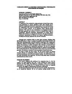
& Reeves, 1997) seem to answer this question in the affirmative: the quality of the local optima generated by this approach was significantly correlated with their distance from a global optimum (where this was known), or with the average distance from other local optima (where a global optimum was not known). In each case, distance was computed by the precedence measure. As an example, Figure 3 shows a scatter plot of local optima for problems ta011 and ta021, being respectively the first of Taillard’s 20 × 10 and 20 × 20 groups of problems (Taillard, 1993). These results were generated by running a stochastic local search as described above with L = 5000 and an acceptance probability using c = 5. The x-axis in Figure 3 represents (a) the average precedence-based distance from other local optima (MEAND), and (b) the precedence-based distance from one of the nearer global optima (BESTD). The y-axis represents their objective function values relative to the global optimum. These plots clearly show that there are good correlations between the distances and objective function values. The calculated correlation coefficients for each plot are: ta011(a): 0.74, ta011(b): 0.50, ta021(a): 0.62 and ta021(b): 0.44. These values are statistically significant at the 0.1% level, on the basis of 1000 replications in a randomization test (Reeves, 1998). These high correlations suggest that the local optima are radially distributed in the problem space relative to a global optimum at the centre; the more distant the local optima are from the centre, the worse are their objective function values. Hence, by tracing local optima step by step, moving from one optimum to a nearby slightly better one, without being trapped, one can hope eventually to reach a near global optimum.

5.3

Mutation

Mutation is nearly always regarded as an integral part of a GA. In this case, we made use of mutation only when parents were too close to each other. In such circumstances, MSXF is not applicable as the number of possible neighbours is severely curtailed—in the limit, where the distance is just one move, there is of course no path at all. In such cases (defined to be when the distance was less than a value dmin ), a mutation operator called Multi-Step Mutation Fusion (MSMF) is applied with the aim of diversifying the search. MSMF can be defined in the same manner as MSXF except that the neighbours of x are sorted in descending order of d(yi , p2 ) in Figure 1, and the most distant solution is stored and used in the next generation instead of q, if q does not improve the parent solutions. As mentioned earlier, (Reeves, 1995) used a purely random scheme to perturb the current population. Here, by contrast, we try to use the structure of the landscape to guide the direction of mutation. From a path relinking viewpoint, we are attempting to extrapolate the path between the solutions, rather than (as normal) to interpolate it.

11

ta011(a)

OBJFN

ta011(b)

OBJFN

140

140

130

130

120

120

110

110

100

100

90

90

80

80

70

70

60

60

50

50

40

40

30

30

20

20

10

10

0

0 40

50

60

70

80

90 MEAND

ta021(a)

OBJFN

0

20

40

80

100

BESTD

ta021(b)

OBJFN

200 190 180 170 160 150 140 130 120 110 100 90 80 70 60 50 40 30 20 10 0

60

200 190 180 170 160 150 140 130 120 110 100 90 80 70 60 50 40 30 20 10 0 70

80

90

100

110 MEAND

0

20

40

60

80

100

120

140

BESTD

Figure 3: 1841 distinct local optima obtained from 2500 short term local search for the ta011 (20 × 10) problem and 2313 distinct local optima for the ta021 (20 × 20) problem are plotted in terms of (a) average distance from other local optima and (b) distance from global optima (x-axis), against their relative objective function values (y-axis).

12

Offspring

Parent2

Parent1

MSXF

Figure 4: Exploration and exploitation: A search is started from one of the parents and while no other good solutions are found, the search traces a path towards the other parent. In the middle of the search, good solutions may be found somewhere between the parents. A local search can then exploit this new starting point by climbing to the top of a hill (or the bottom of a valley, if it is a minimization problem)—a new local optimum.

5.4

Local search

In the initial stages, even the best members of the poulation are unlikely to be local optima. In fact, it is likely that they are in quite the wrong part of the landscape for the big valley hypothesis to hold. It is thus important to incorporate a local search into the algorithm. This enables the fast location of the big valley region in the early stages, but it may also be beneficial later. When points on the path have been selected and inserted into the population, they are probably not local optima either. Rather, they provide good initial points for a local search to exploit. It was decided to make the choice of local search a probabilistic one—with probability PX the algorithm would use path relinking (either interpolatory or extrapolatory), otherwise a stochastic local search was used on the first parent selected. This used a constant temperature Pc for a fixed number of iterations L. In this way a balance can be struck between the exploratory effect of path relinking, and the exploitation of new data by local search. Figure 4 gives a pictorial representation of the idea.

6

Experimental Results

The above ideas were incorporated into a C program and implemented on a DEC Alpha 600 5/226 computer. A template summarizing the final version of the algorithm is given in Figure 5. The parameter values used were as follows (no attempt was made to investigate whether these

13

• Initialize population: randomly generate a set of permutation schedules. Sort the population members in descending order of their makespan values. do 1. Select two schedules p1 , p2 from the population with a probability inversely proportional to their ranks. 2. Do Step (a) with probability PX , otherwise do Step (b). (a) If the precedence-based distance between p1 , p2 is less than dmin , apply MSMF to p1 and generate q. Otherwise, apply MSXF to p1 , p2 using the representative neighbourhood and the precedence-based distance and generate a new schedule q. (b) Apply local search to p1 with acceptance probability Pc and the representative neighbourhood. q is the best solution found during L iterations. 3. If q’s makespan is less than the worst in the population, and no member of the current population has the same makespan as q, replace the worst individual with q. until some termination condition is satisfied. • Output the best schedule in the population.

Figure 5: The GA with embedded path relinking for the PFSP

14

were in any sense ‘optimal’). The population size = 15, constant temperature c = 3, number of iterations for each path relinking or local search phase L = 1000, and dmin = n/2. The probability PX = 0.5. Global optima are now known for all Taillard’s smaller PFSP benchmarks (instances ranging from 20 × 5 to 50 × 10 in size). The algorithm was run on these, and in every case it quite quickly found a solution within about 1% of the global optimum. Of more interest are the larger problem instances, where global optima are still unknown. Table 1 summarizes the performance statistics for a subset of Taillard’s larger benchmarks, together with the results found by Nowicki and Smutnicki using their TS implementation (Nowicki & Smutnicki, 1996) and the lower and upper bounds, taken from the OR-library (Beasley, 1990). (These upper bounds are the currently best-known makespans, most of them found by a branch and bound technique with computational time unknown). In all, 30 runs were completed for each problem under the same conditions but with different random number seeds. Each run was terminated after 700 iterations, which took about 12, 21 and 47 minutes of CPU time respectively for each 50 × 20, 100 × 20 and 200 × 20 problem. It can be seen that the results for 50 × 20 problems are impressive: the solution quality of our best results improves those found in (Nowicki & Smutnicki, 1996) for most of the problems, and some results (marked in bold letters) are even better than the existing best results reported in the OR-library. The results for larger problems are not as good as those for the 50 × 20 problems, but still good enough to support our hypothesis that implementing crossover as path relinking offers an effective way to improve GA performance significantly. It is of interest that the best solutions obtained were (with one exception) within 2% of the lower bound, and often significantly closer; even the mean values were seldom much further distant; finally, the standard deviations were all small, so that the possibility of generating a really poor solution is remote. The degradation that we see as the problem size increases is probably due to the increasing complexity of the neighbourhood calculation. In fact, for problems where the ratio n/m > 3, Nowicki and Smutnicki abandoned their representative neighbourhood and used a simple one instead: just moving a job to the beginning or the end of its critical block. They also implemented an efficient way of evaluating all the members in the neighbourhood in a specific order. This method is useful for the tabu search, but not directly applicable to our approach. Their paper (Nowicki & Smutnicki, 1996) provides more details. Some further experiments were carried out on the 50 × 20 set of instances, where CPU time was increased by a factor of about 4. The results of these experiments (based on 10 replications, rather than 30) are shown in Table 2. It appears from this table that longer runs are able to improve the quality of solution even more—in 6 cases, further new best solutions have been obtained. (Altogether, 7 new best solutions have been found, and in the other cases the difference is either 0 or 1 unit.) Perhaps of almost

15

50 × 20

best

avg

std

nowi

lb – ub

1

3861

3880

9.3

3875

3771–3875

2

3709

3716

2.9

3715

3661–3715

3

3651

3668

6.2

3668

3591–3668

4

3726

3744

6.1

3752

3631–3752

5

3614

3636

8.9

3635

3551–3635

6

3690

3701

6.7

3698

3667–3687

7

3711

3723

5.6

3716

3672–3706

8

3699

3721

7.7

3709

3627–3700

9

3760

3769

5.2

3765

3645–3755

10

3767

3772

4.2

3777

3696–3767

100 × 20

best

avg

std

nowi

lb – ub

1

6242

6259

9.6

6286

6106–6228

2

6217

6234

8.9

6241

6183–6210

3

6299

6312

7.8

6329

6252–6271

4

6288

6303

2.7

6306

6254–6269

5

6329

6354

11.3

6377

6262–6319

6

6380

6417

12.7

6437

6302–6403

7

6302

6319

11.0

6346

6184–6292

8

6433

6466

17.3

6481

6315–6423

9

6297

6323

11.4

6358

6204–6275

0

6448

6471

10.6

6465

6404–6434

200 × 20

best

avg

std

nowi

lb – ub

1

11272

11316

20.8

11294

11152–11195

2

11299

11346

21.4

11420

11143–11223

3

11410

11458

25.2

11446

11281–11337

4

11347

11400

29.9

11347

11275–11299

5

11290

11320

16.6

11311

11259–11260

6

11250

11288

23.4

11282

11176–11189

7

11438

11455

9.3

11456

11337–11386

8

11395

11426

16.4

11415

11301–11334

9

11263

11306

21.5

11343

11145–11192

10

11335

11409

31.3

11422

11284–11313

Table 1: Results of the Taillard benchmark problems: best, avg, std denote the best, average and standard deviation of our 30 makespan values; nowi denotes the results of Nowicki and Smutnicki; lb, ub are the theoretical lower bounds and currently best known makespan values taken from the OR-library; bold figures are those which are better than the current ub. 16

Table 2: Results of longer runs (approx. 45 mins.) for the 50 × 20 instances No.

best

avg. nowi

lb – ub

1 3855 3863 3875 3771–3875 2 3708 3713 3715 3661–3715 3 3647 3657 3668 3591–3668 4 3731 3735 3752 3631–3752 5 3614 3621 3635 3551–3635 6 3686 3692 3698 3667–3687 7 3707 3713 3716 3672–3706 8 3701 3712 3709 3627–3700 9 3743 3761 3765 3645–3755 10 3767 3768 3777 3696–3767

equal significance is the very good average performance, which in many cases is within a few units of the best. This suggests that the result of just a single long run is likely to be very close to the global optimum.

7

Conclusions

The concept of path relinking has been introduced as a means of enhancing the performance of a GA for the permutation flowshop scheduling problem. Empirical analysis using 20 × 10 and 20 × 20 Taillard benchmark problems has confirmed the existence of a ‘big valley’ structure which motivates the use of such techniques. A GA for the PFSP has therefore been implemented using the representative neighbourhood and path relinking, and applied to more challenging benchmark problems. Experimental results demonstrate the effectiveness of the proposed method, and several new upper bound values have been found for Taillard’s benchmarks. Further investigation will be carried out to examine whether it is possible to reduce the computational time further without losing the quality of solution found in this work. It is also planned to investigate different types of flowshop problem, such as the minimization of the sum of job completion times, and those with more complex requirements such as sequence dependent setup times, and to explore alternative ways of implementing path relinking. It should also be pointed out that other combinatorial problems such as graph bisection and the TSP have also been found to possess a ‘big valley’ structure. If this is a feature of many COPs, we would expect a genetic algorithm with embedded path relinking to prove a fruitful approach to its solution, so that the findings of this paper might well be of more general relevance.

17

References Beasley, J. (1990).

Or-library:

Distributing test problems by electronic mail.

European

J.Operational Research, 41, 1069–1072. Boese, K., Kahng, A., & Muddu, S. (1994). A new adaptive multi-start technique for combinatorial global optimizations. Ops.Res. Letters, 16, 101–113. Cartwright, H. & Tuson, A. (1994). Genetic algorithms and flowshop scheduling: towards the development of a real-time process control system. In Evolutionary Computing: AISB Workshop, Leeds, UK, April 1994; Selected Papers (pp. 277–290). Berlin: Springer-Verlag. Culberson, J. (1995). Mutation-crossover isomorphisms and the construction of discriminating functions. Evolutionary Computation, 2, 279–311. Davis, L. (1985). Job shop scheduling with genetic algorithms. In Proceedings of an International Conference on Genetic Algorithms and Their Applications (pp. 136–140). Hillsdale, New Jersey: Lawrence Erlbaum Associates. Garey, M. & Johnson, D. (1979). Computers and Intractibility: A Guide to the Theory of NPCompleteness. San Francisco: W.H.Freeman. Glover, F. & Laguna, M. (1993). Tabu Search. Chapter 3 in Modern Heuristic Techniques for Combinatorial Problems. Blackwell Scientific Publications: Oxford. (Recently re-issued (1995) by McGraw-Hill, London.). Goldberg, D. & Lingle, R. (1985). Alleles, loci and the traveling salesman problem. In Proceedings of an International Conference on Genetic Algorithms and Their Applications (pp. 154–159). Hillsdale, New Jersey: Lawrence Erlbaum Associates. H¨ohn, C. & Reeves, C. (1996a). Are long path problems hard for genetic algorithms? In Parallel Problem-Solving from Nature-PPSN IV (pp. 134–143). Berlin: Springer-Verlag. H¨ohn, C. & Reeves, C. (1996b). The crossover landscape for the onemax problem. In Proceedings of the 2nd Nordic Workshop on Genetic Algorithms and their Applications (pp. 27–43). Vaasa, Finland: University of Vaasa Press. Johnson, D. (1990). Local optimization and the traveling salesman problem. Automata, Languages and Programming, Lecture Notes in Computer Science, 443, 446–461. Jones, T. (1995). Evolutionary Algorithms, Fitness Landscapes and Search. PhD thesis, University of New Mexico, Albuquerque, NM. Kauffman, S. (1993). The Origins of Order: Self-Organisation and Selection in Evolution. Oxford University Press. 18

Nawaz, M., Emscore Jr., E., & Ham, I. (1983). A heuristic algorithm for the m-machine, n-job flow-shop sequencing problem. OMEGA, 11, 91–95. Nowicki, E. & Smutnicki, C. (1996). A fast tabu search algorithm for the permutation flow-shop problem. European J.Operational Research, 91, 160–175. Ogbu, F. & Smith, D. (1990). The application of the simulated annealing algorithm to the solution of the n/m/Cmax flowshop problem. Computers & Operations Research, 17, 243–253. Ogbu, F. & Smith, D. (1991).

Simulated annealing for the permutation flow-shop problem.

OMEGA, 19, 64–67. Osman, I. & Potts, C. (1989). Simulated annealing for permutation flow-shop scheduling. OMEGA, 17, 551–557. Rana, S. & Whitley, D. (1997). Bit representation with a twist. In Proceedings of the 7th International Conference on Genetic Algorithms (pp. 188–195). San Francisco, CA: Morgan Kaufmann. Reeves, C. (1992). A genetic algorithm approach to stochastic flowshop sequencing. In Proc.IEE Colloquium on Genetic Algorithms for Control and Systems Engineering, London, UK: IEE. Digest No.1992/106. Reeves, C. (1993).

Improving the efficiency of tabu search in machine sequencing problems.

J.Opl.Res.Soc., 44, 375–382. Reeves, C. (1994). Genetic algorithms and neighbourhood search. In Evolutionary Computing: AISB Workshop, Leeds, UK, April 1994; Selected Papers (pp. 115–130). Berlin: SpringerVerlag. Reeves, C. (1995). A genetic algorithm for flowshop sequencing. Computers & Operations Research, 22, 5–13. Reeves, C. (1998). Landscapes, operators and heuristic search. Annals of Operations Research. To appear. Reeves, C. & Karatza, H. (1993). An experimental investigation of a multi-processor scheduling system. In G.Nemeth (Ed.) Proc. Workshop on Computer Performance Evaluation, Architectures and Scheduling, Hungary: Technical University of Budapest. Rinnooy Kan, A. (1976). Machine Scheduling Problems: Classification, Complexity and Computations. The Hague: Martinus Nijhoff. Taillard, E. (1990).

Some efficient heuristic methods for the flow shop sequencing problem.

Euro.J.Operational Research, 47, 65–74. 19

Taillard, E. (1993). Benchmarks for basic scheduling problems. Euro.J.Operational Research, 64, 278–285. Vaessens, R. (1995). Personal communication. Widmer, M. & Hertz, A. (1989). A new heuristic method for the flow shop sequencing problem. Euro.J.Operational Research, 41, 186–193. Yamada, T. & Nakano, R. (1996). Scheduling by genetic local search with multi-step crossover. In Parallel Problem-Solving from Nature-PPSN IV (pp. 960–969). Berlin: Springer-Verlag. Yamada, T. & Reeves, C. (1997). Permutation flowshop scheduling by genetic local search. In Proceedings of the 2nd IEE/IEEE International Conference on Genetic ALgorithms in Engineering Systems (GALESIA ’97) (pp. 232–238). London, UK: IEE. Yamada, T. & Reeves, C. (1998). Distance measures in the permutation flowshop problem. Work in progress.

20