Geometric deep learning: going beyond Euclidean data - arXiv

IEEE SIG PROC MAG

1

Geometric deep learning: going beyond Euclidean data

arXiv:1611.08097v2 [cs.CV] 3 May 2017

Michael M. Bronstein, Joan Bruna, Yann LeCun, Arthur Szlam, Pierre Vandergheynst

Many scientific fields study data with an underlying structure that is a non-Euclidean space. Some examples include social networks in computational social sciences, sensor networks in communications, functional networks in brain imaging, regulatory networks in genetics, and meshed surfaces in computer graphics. In many applications, such geometric data are large and complex (in the case of social networks, on the scale of billions), and are natural targets for machine learning techniques. In particular, we would like to use deep neural networks, which have recently proven to be powerful tools for a broad range of problems from computer vision, natural language processing, and audio analysis. However, these tools have been most successful on data with an underlying Euclidean or grid-like structure, and in cases where the invariances of these structures are built into networks used to model them. Geometric deep learning is an umbrella term for emerging techniques attempting to generalize (structured) deep neural models to non-Euclidean domains such as graphs and manifolds. The purpose of this paper is to overview different examples of geometric deep learning problems and present available solutions, key difficulties, applications, and future research directions in this nascent field. I. I NTRODUCTION “Deep learning” refers to learning complicated concepts by building them from simpler ones in a hierarchical or multi-layer manner. Artificial neural networks are popular realizations of such deep multi-layer hierarchies. In the past few years, the growing computational power of modern GPUbased computers and the availability of large training datasets have allowed successfully training neural networks with many layers and degrees of freedom [1]. This has led to qualitative breakthroughs on a wide variety of tasks, from speech recognition [2], [3] and machine translation [4] to image analysis and computer vision [5], [6], [7], [8], [9], [10], [11] (the reader is referred to [12], [13] for many additional examples of successful applications of deep learning). Nowadays, deep learning has matured into a technology that is widely used in commercial applications, including Siri speech recognition in Apple iPhone, Google text translation, and Mobileye visionbased technology for autonomously driving cars. One of the key reasons for the success of deep neural networks is their ability to leverage statistical properties of MB is with USI Lugano, Switzerland, Tel Aviv University, and Intel Perceptual Computing, Israel. JB is with Courant Institute, NYU and UC Berkeley, USA. YL with with Facebook AI Research and NYU, USA. AS is with Facebook AI Research, USA. PV is with EPFL, Switzerland.

the data such as stationarity and compositionality through local statistics, which are present in natural images, video, and speech [14], [15]. These statistical properties have been related to physics [16] and formalized in specific classes of convolutional neural networks (CNNs) [17], [18], [19]. In image analysis applications, one can consider images as functions on the Euclidean space (plane), sampled on a grid. In this setting, stationarity is owed to shift-invariance, locality is due to the local connectivity, and compositionality stems from the multi-resolution structure of the grid. These properties are exploited by convolutional architectures [20], which are built of alternating convolutional and downsampling (pooling) layers. The use of convolutions has a two-fold effect. First, it allows extracting local features that are shared across the image domain and greatly reduces the number of parameters in the network with respect to generic deep architectures (and thus also the risk of overfitting), without sacrificing the expressive capacity of the network. Second, the convolutional architecture itself imposes some priors about the data, which appear very suitable especially for natural images [21], [18], [17], [19]. While deep learning models have been particularly successful when dealing with signals such as speech, images, or video, in which there is an underlying Euclidean structure, recently there has been a growing interest in trying to apply learning on non-Euclidean geometric data. Such kinds of data arise in numerous applications. For instance, in social networks, the characteristics of users can be modeled as signals on the vertices of the social graph [22]. Sensor networks are graph models of distributed interconnected sensors, whose readings are modelled as time-dependent signals on the vertices. In genetics, gene expression data are modeled as signals defined on the regulatory network [23]. In neuroscience, graph models are used to represent anatomical and functional structures of the brain. In computer graphics and vision, 3D objects are modeled as Riemannian manifolds (surfaces) endowed with properties such as color texture. The non-Euclidean nature of such data implies that there are no such familiar properties as global parameterization, common system of coordinates, vector space structure, or shift-invariance. Consequently, basic operations like convolution that are taken for granted in the Euclidean case are even not well defined on non-Euclidean domains. The purpose of our paper is to show different methods of translating the key ingredients of successful deep learning methods such as convolutional neural networks to non-Euclidean data.

IEEE SIG PROC MAG

II. G EOMETRIC LEARNING PROBLEMS Broadly speaking, we can distinguish between two classes of geometric learning problems. In the first class of problems, the goal is to characterize the structure of the data. The second class of problems deals with analyzing functions defined on a given non-Euclidean domain. These two classes are related, since understanding the properties of functions defined on a domain conveys certain information about the domain, and vice-versa, the structure of the domain imposes certain properties on the functions on it. Structure of the domain: As an example of the first class of problems, assume to be given a set of data points with some underlying lower dimensional structure embedded into a high-dimensional Euclidean space. Recovering that lower dimensional structure is often referred to as manifold learning1 or non-linear dimensionality reduction, and is an instance of unsupervised learning. Many methods for nonlinear dimensionality reduction consist of two steps: first, they start with constructing a representation of local affinity of the data points (typically, a sparsely connected graph). Second, the data points are embedded into a low-dimensional space trying to preserve some criterion of the original affinity. For example, spectral embeddings tend to map points with many connections between them to nearby locations, and MDS-type methods try to preserve global information such as graph geodesic distances. Examples of manifold learning include different flavors of multidimensional scaling (MDS) [26], locally linear embedding (LLE) [27], stochastic neighbor embedding (t-SNE) [28], spectral embeddings such as Laplacian eigenmaps [29] and diffusion maps [30], and deep models [31]. Most recent approaches [32], [33], [34] tried to apply the successful word embedding model [35] to graphs. Instead of embedding the vertices, the graph structure can be processed by decomposing it into small sub-graphs called motifs [36] or graphlets [37]. In some cases, the data are presented as a manifold or graph at the outset, and the first step of constructing the affinity structure described above is unnecessary. For instance, in computer graphics and vision applications, one can analyze 3D shapes represented as meshes by constructing local geometric descriptors capturing e.g. curvature-like properties [38], [39]. In network analysis applications such as computational sociology, the topological structure of the social graph representing the social relations between people carries important insights allowing, for example, to classify the vertices and detect communities [40]. In natural language processing, words in a corpus can be represented by the co-occurrence graph, where two words are connected if they often appear near each other [41]. Data on a domain: Our second class of problems deals with analyzing functions defined on a given non-Euclidean domain. We can further break down such problems into two subclasses: problems where the domain is fixed and those where multiple domains are given. For example, assume that we are given the geographic coordinates of the users of a social network, 1 Note

that the notion of “manifold” in this setting can be considerably more general than a classical smooth manifold; see e.g. [24], [25]

2

represented as a time-dependent signal on the vertices of the social graph. An important application in location-based social networks is to predict the position of the user given his or her past behavior, as well as that of his or her friends [42]. In this problem, the domain (social graph) is assumed to be fixed; methods of signal processing on graphs, which have previously been reviewed in this Magazine [43], can be applied to this setting, in particular, in order to define an operation similar to convolution in the spectral domain. This, in turn, allows generalizing CNN models to graphs [44], [45]. In computer graphics and vision applications, finding similarity and correspondence between shapes are examples of the second sub-class of problems: each shape is modeled as a manifold, and one has to work with multiple such domains. In this setting, a generalization of convolution in the spatial domain using local charting [46], [47], [48] appears to be more appropriate. Brief history: The main focus of this review is on this second class of problems, namely learning functions on nonEuclidean structured domains, and in particular, attempts to generalize the popular CNNs to such settings. First attempts to generalize neural networks to graphs we are aware of are due to Scarselli et al. [49], who proposed a scheme combining recurrent neural networks and random walk models. This approach went almost unnoticed, re-emerging in a modern form in [50], [51] due to the renewed recent interest in deep learning. The first formulation of CNNs on graphs is due to Bruna et al. [52], who used the definition of convolutions in the spectral domain. Their paper, while being of conceptual importance, came with significant computational drawbacks that fell short of a truly useful method. These drawbacks were subsequently addressed in the followup works of Henaff et al. [44] and Defferrard et al. [45]. In the latter paper, graph CNNs allowed achieving some state-of-the-art results. In a parallel effort in the computer vision and graphics community, Masci et al. [47] showed the first CNN model on meshed surfaces, resorting to a spatial definition of the convolution operation based on local intrinsic patches. Among other applications, such models were shown to achieve stateof-the-art performance in finding correspondence between deformable 3D shapes. Followup works proposed different construction of intrinsic patches on point clouds [53], [48] and general graphs [54]. The interest in deep learning on graphs or manifolds has exploded in the past year, resulting in numerous attempts to apply these methods in a broad spectrum of problems ranging from biochemistry [55] to recommender systems [56]. Since such applications originate in different fields that usually do not cross-fertilize, publications in this domain tend to use different terminology and notation, making it difficult for a newcomer to grasp the foundations and current state-of-the-art methods. We believe that our paper comes at the right time attempting to systemize and bring some order into the field. Structure of the paper: We start with an overview of traditional Euclidean deep learning in Section III, summarizing the important assumptions about the data, and how they are

IEEE SIG PROC MAG

3

realized in convolutional network architectures.2 Going to the non-Euclidean world in Section IV, we then define basic notions in differential geometry and graph theory. These topics are insufficiently known in the signal processing community, and to our knowledge, there is no introductorylevel reference treating these so different structures in a common way. One of our goals is to provide an accessible overview of these models resorting as much as possible to the intuition of traditional signal processing. In Sections V–VIII, we overview the main geometric deep learning paradigms, emphasizing the similarities and the differences between Euclidean and non-Euclidean learning methods. The key difference between these approaches is in the way a convolution-like operation is formulated on graphs and manifolds. One way is to resort to the analogy of the Convolution Theorem, defining the convolution in the spectral domain. An alternative is to think of the convolution as a template matching in the spatial domain. Such a distinction is, however, far from being a clear-cut: as we will see, some approaches though draw their formulation from the spectral domain, essentially boil down to applying filters in the spatial domain. It is also possible to combine these two approaches resorting to spatio-frequency analysis techniques, such as wavelets or the windowed Fourier transform. In Section IX, we show examples of selected problems from the fields of network analysis, particle physics, recommender systems, computer vision, and graphics. In Section X, we draw conclusions and outline current main challenges and potential future research directions in geometric deep learning. To make the paper more readable, we use inserts to illustrate important concepts. Finally, the readers are invited to visit a dedicated website geometricdeeplearning.com for additional materials, data, and examples of code.

Notation Rm a, a, A a ¯ Ω, x f ∈ L2 (Ω) δx0 (x), δij {fi , yi }i∈I Tv τ, Lτ fˆ f ?g X , T X , Tx X h·, ·, iT X f ∈ L2 (X ) F ∈ L2 (T X ) A∗ ∇, div, ∆ V, E, F wij , W f ∈ L2 (V) F ∈ L2 (E) φi , λi ht (·, ·) Φk Λk ξ γl,l0 (x), Γl,l0

m-dimensional Euclidean space Scalar, vector, matrix Complex conjugate of a Arbitrary domain, coordinate on it Square-integrable function on Ω Delta function at x0 , Kronecker delta Training set Translation operator Deformation field, operator Fourier transform of f Convolution of f and g Manifold, its tangent bundle, tangent space at x Riemannian metric Scalar field on manifold X Tangent vector field on manifold X Adjoint of operator A Gradient, divergence, Laplace operators Vertices and edges of a graph, faces of a mesh Weight matrix of a graph, Functions on vertices of a graph Functions on edges of a graph Laplacian eigenfunctions, eigenvalues Heat kernel Matrix of first k Laplacian eigenvectors Diagonal matrix of first k Laplacian eigenvalues Point-wise nonlinearity (e.g. ReLU) Convolutional filter in spatial and spectral domain

III. D EEP LEARNING ON E UCLIDEAN DOMAINS Geometric priors: Consider a compact d-dimensional Euclidean domain Ω = [0, 1]d ⊂ Rd on which squareintegrable functions f ∈ L2 (Ω) are defined (for example, in image analysis applications, images can be thought of as functions on the unit square Ω = [0, 1]2 ). We consider a generic supervised learning setting, in which an unknown function y : L2 (Ω) → Y is observed on a training set

Stationarity: Let Tv f (x) = f (x − v),

x, v ∈ Ω,

(2)

In a supervised classification setting, the target space Y can be thought discrete with |Y| being the number of classes. In a multiple object recognition setting, we can replace Y by the K-dimensional simplex, which represents the posterior class probabilities p(y|x). In regression tasks, we may consider Y = Rm . In the vast majority of computer vision and speech analysis tasks, there are several crucial prior assumptions on the unknown function y. As we will see in the following, these assumptions are effectively exploited by convolutional neural network architectures.

be a translation operator3 acting on functions f ∈ L2 (Ω). Our first assumption is that the function y is either invariant or equivariant with respect to translations, depending on the task. In the former case, we have y(Tv f ) = y(f ) for any f ∈ L2 (Ω) and v ∈ Ω. This is typically the case in object classification tasks. In the latter, we have y(Tv f ) = Tv y(f ), which is welldefined when the output of the model is a space in which translations can act upon (for example, in problems of object localization, semantic segmentation, or motion estimation). Our definition of invariance should not be confused with the traditional notion of translation invariant systems in signal processing, which corresponds to translation equivariance in our language (since the output translates whenever the input translates). Local deformations and scale separation: Similarly, a deformation Lτ , where τ : Ω → Ω is a smooth vector field, acts on L2 (Ω) as Lτ f (x) = f (x − τ (x)). Deformations can

2 For a more in-depth review of CNNs and their applications, we refer the reader to [12], [1], [13] and references therein.

3 We assume periodic boundary conditions to ensure that the operation is well-defined over L2 (Ω).

{fi ∈ L2 (Ω), yi = y(fi )}i∈I .

(1)

IEEE SIG PROC MAG

4

model local translations, changes in point of view, rotations and frequency transpositions [18]. Most tasks studied in computer vision are not only translation invariant/equivariant, but also stable with respect to local deformations [57], [18]. In tasks that are translation invariant we have |y(Lτ f ) − y(f )| ≈ k∇τ k, (3)

Additionally, a downsampling or pooling layer g = P (f ) may be used, defined as gl (x) = P ({fl (x0 ) : x0 ∈ N (x)}), l = 1, . . . , q,

(8)

for all f, τ . Here, k∇τ k measures the smoothness of a given deformation field. In other words, the quantity to be predicted does not change much if the input image is slightly deformed. In tasks that are translation equivariant, we have

where N (x) ⊂ Ω is a neighborhood around x and P is a permutation-invariant function such as a Lp -norm (in the latter case, the choice of p = 1, 2 or ∞ results in average-, energy-, or max-pooling). A convolutional network is constructed by composing several convolutional and optionally pooling layers, obtaining a generic hierarchical representation

|y(Lτ f ) − Lτ y(f )| ≈ k∇τ k.

UΘ (f ) = (CΓ(K) · · · P · · · ◦ CΓ(2) ◦ CΓ(1) )(f )

(4)

This property is much stronger than the previous one, since the space of local deformations has a high dimensionality, as opposed to the d-dimensional translation group. It follows from (3) that we can extract sufficient statistics at a lower spatial resolution by downsampling demodulated localized filter responses without losing approximation power. An important consequence of this is that long-range dependencies can be broken into multi-scale local interaction terms, leading to hierarchical models in which spatial resolution is progressively reduced. To illustrate this principle, denote by Y (x1 , x2 ; v) = Prob(f (u) = x1 and f (u + v) = x2 ) (5) the joint distribution of two image pixels at an offset v from each other. In the presence of long-range dependencies, this joint distribution will not be separable for any v. However, the deformation stability prior states that Y (x1 , x2 ; v) ≈ Y (x1 , x2 ; v(1 + )) for small . In other words, whereas long-range dependencies indeed exist in natural images and are critical to object recognition, they can be captured and down-sampled at different scales. This principle of stability to local deformations has been exploited in the computer vision community in models other than CNNs, for instance, deformable parts models [58]. In practice, the Euclidean domain Ω is discretized using a regular grid with n points; the translation and deformation operators are still well-defined so the above properties hold in the discrete setting. Convolutional neural networks: Stationarity and stability to local translations are both leveraged in convolutional neural networks (see insert IN1). A CNN consists of several convolutional layers of the form g = CΓ (f ), acting on a pdimensional input f (x) = (f1 (x), . . . , fp (x)) by applying a bank of filters Γ = (γl,l0 ), l = 1, . . . , q, l0 = 1, . . . , p and point-wise non-linearity ξ, ! p X gl (x) = ξ (fl0 ? γl,l0 )(x) , (6) l0 =1

producing a q-dimensional output g(x) = (g1 (x), . . . , gq (x)) often referred to as the feature maps. Here, Z (f ? γ)(x) = f (x − x0 )γ(x0 )dx0 (7) Ω

denotes the standard convolution. According to the local deformation prior, the filters Γ have compact spatial support.

(9)

where Θ = {Γ(1) , . . . , Γ(K) } is the hyper-vector of the network parameters (all the filter coefficients). The model is said to be deep if it comprises multiple layers, though this notion is rather vague and one can find examples of CNNs with as few as a couple and as many as hundreds of layers [11]. The output features enjoy translation invariance/covariance depending on whether spatial resolution is progressively lost by means of pooling or kept fixed. Moreover, if one specifies the convolutional tensors to be complex wavelet decomposition operators and uses complex modulus as pointwise nonlinearities, one can provably obtain stability to local deformations [17]. Although this stability is not rigorously proved for generic compactly supported convolutional tensors, it underpins the empirical success of CNN architectures across a variety of computer vision applications [1]. In supervised learning tasks, one can obtain the CNN parameters by minimizing a task-specific cost L on the training set {fi , yi }i∈I , X min L(UΘ (fi ), yi ), (10) Θ

i∈I

for instance, L(x, y) = kx − yk. If the model is sufficiently complex and the training set is sufficiently representative, when applying the learned model to previously unseen data, one expects U (f ) ≈ y(f ). Although (10) is a non-convex optimization problem, stochastic optimization methods offer excellent empirical performance. Understanding the structure of the optimization problems (10) and finding efficient strategies for its solution is an active area of research in deep learning [62], [63], [64], [65], [66]. A key advantage of CNNs explaining their success in numerous tasks is that the geometric priors on which CNNs are based result in a learning complexity that avoids the curse of dimensionality. Thanks to the stationarity and local deformation priors, the linear operators at each layer have a constant number of parameters, independent of the input size n (number of pixels in an image). Moreover, thanks to the multiscale hierarchical property, the number of layers grows at a rate O(log n), resulting in a total learning complexity of O(log n) parameters. IV. T HE GEOMETRY OF MANIFOLDS AND GRAPHS Our main goal is to generalize CNN-type constructions to non-Euclidean domains. In this paper, by non-Euclidean

IEEE SIG PROC MAG

5

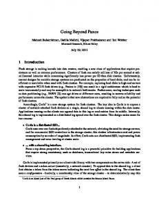
[IN1] Convolutional neural networks: CNNs are currently among the most successful deep learning architectures in a variety of tasks, in particular, in computer vision. A typical CNN used in computer vision applications (see FIGS1) consists of multiple convolutional layers (6), passing the input image through a set of filters Γ followed by point-wise nonlinearity ξ (typically, half-rectifiers ξ(z) = max(0, z) are used, although practitioners have experimented with a diverse range of choices [13]). The model can also include a bias term, which is equivalent to adding a constant coordinate to the input. A network composed of K convolutional layers put together U (f ) = (CΓ(K) . . . ◦ CΓ(2) ◦ CΓ(1) )(f ) produces pixel-wise features that are covariant w.r.t. translation and approximately covariant to local deformations. Typical computer vision appli-

cations requiring covariance are semantic image segmentation [8] or motion estimation [59]. In applications requiring invariance, such as image classification [7], the convolutional layers are typically interleaved with pooling layers (8) progressively reducing the resolution of the image passing through the network. Alternatively, one can integrate the convolution and downsampling in a single linear operator (convolution with stride). Recently, some authors have also experimented with convolutional layers which increase the spatial resolution using interpolation kernels [60]. These kernels can be learnt efficiently by mimicking the socalled algorithme a` trous [61], also referred to as dilated convolution.

Samoyed (16) ; Papillon (5.7) ; Pomeranzian (2.7) ; Arctic fox (1.0) ; Eskimo dog (0.6) ; White wolf (0.4) ; Siberian husky (0.4)

Convolutions and ReLU Max pooling

Convolutions and ReLU Max pooling

Convolutions and ReLU

Red

Green

Blue

[FIGS1] Typical convolutional neural network architecture used in computer vision applications (figure reproduced from [1]).

domains, we refer to two prototypical structures: manifolds and graphs. While arising in very different fields of mathematics (differential geometry and graph theory, respectively), in our context, these structures share several common characteristics that we will try to emphasize throughout our review. Manifolds: Roughly, a manifold is a space that is locally Euclidean. One of the simplest examples is a spherical surface modeling our planet: around a point, it seems to be planar, which has led generations of people to believe in the flatness of the Earth. Formally speaking, a (differentiable) d-dimensional manifold X is a topological space where each point x has a neighborhood that is topologically equivalent (homeomorphic) to a d-dimensional Euclidean space, called the tangent space and denoted by Tx X (see Figure 1, top). The collection of tangent spaces at all points (more formally, their disjoint union) is referred to as the tangent bundle and denoted by T X . On each tangent space, we define an inner product h·, ·iTx X : Tx X × Tx X → R, which is additionally assumed to depend smoothly on the position x. This inner product

is called a Riemannian metric in differential geometry and allows performing local measurements of angles, distances, and volumes. A manifold equipped with a metric is called a Riemannian manifold. It is important to note that the definition of a Riemannian manifold is completely abstract and does not require a geometric realization in any space. However, a Riemannian manifold can be realized as a subset of a Euclidean space (in which case it is said to be embedded in that space) by using the structure of the Euclidean space to induce a Riemannian metric. The celebrated Nash Embedding Theorem guarantees that any sufficiently smooth Riemannian manifold can be realized in a Euclidean space of sufficiently high dimension [67]. An embedding is not necessarily unique; two different realizations of a Riemannian metric are called isometries. Two-dimensional manifolds (surfaces) embedded into R3 are used in computer graphics and vision to describe boundary surfaces of 3D objects, colloquially referred to as ‘3D shapes’. This term is somewhat misleading since ‘3D’ here refers to the

IEEE SIG PROC MAG

6

Tx X

F (x) x F (x0 ) x0 Tx0 X

Fig. 1. Top: tangent space and tangent vectors on a two-dimensional manifold (surface). Bottom: Examples of isometric deformations.

dimensionality of the embedding space rather than that of the manifold. Thinking of such a shape as made of infinitely thin material, inelastic deformations that do not stretch or tear it are isometric. Isometries do not affect the metric structure of the manifold and consequently, preserve any quantities that can be expressed in terms of the Riemannian metric (called intrinsic). Conversely, properties related to the specific realization of the manifold in the Euclidean space are called extrinsic. As an intuitive illustration of this difference, imagine an insect that lives on a two-dimensional surface (Figure 1, bottom). A human observer, on the other hand, sees a surface in 3D space - this is an extrinsic point of view. Calculus on manifolds: Our next step is to consider functions defined on manifolds. We are particularly interested in two types of functions: A scalar field is a smooth real function f : X → R on the manifold. A tangent vector field F : X → T X is a mapping attaching a tangent vector F (x) ∈ Tx X to each point x. As we will see in the following, tangent vector fields are used to formalize the notion of infinitesimal displacements on the manifold. We define the Hilbert spaces of scalar and vector fields on manifolds, denoted by L2 (X ) and L2 (T X ), respectively, with the following inner products: Z hf, giL2 (X ) = f (x)g(x)dx; (15) ZX hF, GiL2 (T X ) = hF (x), G(x)iTx X dx; (16) X

dx denotes here a d-dimensional volume element induced by the Riemannian metric. In calculus, the notion of derivative describes how the value of a function changes with an infinitesimal change of its argument. One of the big differences distinguishing classical calculus from differential geometry is a lack of vector space

structure on the manifold, prohibiting us from na¨ıvely using expressions like f (x+dx). The conceptual leap that is required to generalize such notions to manifolds is the need to work locally in the tangent space. To this end, we define the differential of f as an operator df : T X → R acting on tangent vector fields. At each point x, the differential can be defined as a linear functional (1-form) df (x) = h∇f (x), · iTx X acting on tangent vectors F (x) ∈ Tx X , which model a small displacement around x. The change of the function value as the result of this displacement is given by applying the form to the tangent vector, df (x)F (x) = h∇f (x), F (x)iTx X , and can be thought of as an extension of the notion of the classical directional derivative. The operator ∇f : L2 (X ) → L2 (T X ) in the definition above is called the intrinsic gradient, and is similar to the classical notion of the gradient defining the direction of the steepest change of the function at a point, with the only difference that the direction is now a tangent vector. Similarly, the intrinsic divergence is an operator div : L2 (T X ) → L2 (X ) acting on tangent vector fields and (formal) adjoint to the gradient operator [71], hF, ∇f iL2 (T X ) = h∇∗ F, f iL2 (X ) = h−divF, f iL2 (X ) . (17) Physically, a tangent vector field can be thought of as a flow of material on a manifold. The divergence measures the net flow of a field at a point, allowing to distinguish between field ‘sources’ and ‘sinks’. Finally, the Laplacian (or Laplace-Beltrami operator in differential geometric jargon) ∆ : L2 (X ) → L2 (X ) is an operator ∆f = −div(∇f )

(18)

acting on scalar fields. Employing relation (17), it is easy to see that the Laplacian is self-adjoint (symmetric), h∇f, ∇f iL2 (T X ) = h∆f, f iL2 (X ) = hf, ∆f iL2 (X ) .

(19)

The lhs in equation (19) is known as the Dirichlet energy in physics and measures the smoothness of a scalar field on the manifold (see insert IN3). The Laplacian can be interpreted as the difference between the average of a function on an infinitesimal sphere around a point and the value of the function at the point itself. It is one of the most important operators in mathematical physics, used to describe phenomena as diverse as heat diffusion (see insert IN4), quantum mechanics, and wave propagation. As we will see in the following, the Laplacian plays a center role in signal processing and learning on non-Euclidean domains, as its eigenfunctions generalize the classical Fourier bases, allowing to perform spectral analysis on manifolds and graphs. It is important to note that all the above definitions are coordinate free. By defining a basis in the tangent space, it is possible to express tangent vectors as d-dimensional vectors and the Riemannian metric as a d × d symmetric positivedefinite matrix. Graphs and discrete differential operators: Another type of constructions we are interested in are graphs, which are popular models of networks, interactions, and similarities

IEEE SIG PROC MAG

7

j

j k α ij aijk

sisting of small triangles glued together. The triplet (V, E, F) is referred to as triangular mesh. To be a correct discretization βij h of a manifold (a manifold mesh), every edge must be shared by ai exactly two triangular faces; if the manifold has a boundary, i i any boundary edge must belong to exactly one triangle. On a triangular mesh, the simplest discretization of the Riemannian metric is given by assigning each edge a length `ij > 0, which must additionally satisfy the triangle inequality in every triangular face. The mesh Laplacian is given by Triangular mesh Undirected graph [FIGS2] Two commonly used discretizations of a two-dimensional formula (25) with wij

`ij

manifold: a graph and a triangular mesh.

[IN2] Laplacian on discrete manifolds: In computer graphics and vision applications, two-dimensional manifolds are commonly used to model 3D shapes. There are several common ways of discretizing such manifolds. First, the manifold is assumed to be sampled at n points. Their embedding coordinates x1 , . . . , xn are referred to as point cloud. Second, a graph is constructed upon these points, acting as its vertices. The edges of the graph represent the local connectivity of the manifold, telling whether two points belong to a neighborhood or not, e.g. with Gaussian edge weights wij = e−kxi −xj k

2

/2σ 2

.

(11)

This simplest discretization, however, does not capture correctly the geometry of the underlying continuous manifold (for example, the graph Laplacian would typically not converge to the continuous Laplacian operator of the manifold with the increase of the sampling density [68]). A geometrically consistent discretization is possible with an additional structure of faces F ∈ V × V × V, where (i, j, k) ∈ F implies (i, j), (i, k), (k, j) ∈ E. The collection of faces represents the underlying continuous manifold as a polyhedral surface con-

between different objects. For simplicity, we will consider weighted undirected graphs, formally defined as a pair (V, E), where V = {1, . . . , n} is the set of n vertices, and E ⊆ V × V is the set of edges, where the graph being undirected implies that (i, j) ∈ E iff (j, i) ∈ E. Furthermore, we associate a weight ai > 0 with each vertex i ∈ V, and a weight wij ≥ 0 with each edge (i, j) ∈ E. Real functions f : V → R and F : E → R on the vertices and edges of the graph, respectively, are roughly the discrete analogy of continuous scalar and tangent vector fields in differential geometry.4 We can define Hilbert spaces L2 (V) and L2 (E) of such functions by specifying the respective inner products, X hf, giL2 (V) = ai fi gi ; (20) i∈V

hF, GiL2 (E)

=

X

wij Fij Gij .

(21)

i∈E 2

Let f ∈ L (V) and F ∈ L2 (E) be functions on the 4 It

is tacitly assumed here that F is alternating, i.e., Fij = −Fji .

wij

=

ai

=

−`2ij + `2jh + `2ih −`2ij + `2jk + `2ik + ; 8aijk 8aijh X 1 aijk , 3

(12) (13)

jk:(i,j,k)∈F

p where aijk = sijk (sijk − `ij )(sijk − `jk )(sijk − `ik ) is the area of triangle ijk given by the Heron formula, and sijk = 21 (`ij + `jk + `ki ) is the semi-perimeter of triangle ijk. The vertex weight ai is interpreted as the local area element (shown in red in FIGS2). Note that the weights (1213) are expressed solely in terms of the discrete metric ` and are thus intrinsic. When the mesh is infinitely refined under some technical conditions, such a construction can be shown to converge to the continuous Laplacian of the underlying manifold [69]. An embedding of the mesh (amounting to specifying the vertex coordinates x1 , . . . , xn ) induces a discrete metric `ij = kxi − xj k2 , whereby (12) become the cotangent weights wij =

1 2

(cot αij + cot βij )

(14)

ubiquitously used in computer graphics [70].

vertices and edges of the graphs, respectively. We can define differential operators acting on such functions analogously to differential operators on manifolds [72]. The graph gradient is an operator ∇ : L2 (V) → L2 (E) mapping functions defined on vertices to functions defined on edges, (∇f )ij

=

fi − fj ,

(22)

automatically satisfying (∇f )ij = −(∇f )ji . The graph divergence is an operator div : L2 (E) → L2 (V) doing the converse, 1 X wij Fij . (23) (divF )i = ai j:(i,j)∈E

It is easy to verify that the two operators are adjoint w.r.t. the inner products (20)–(21), hF, ∇f iL2 (E) = h∇∗ F, f iL2 (V) = h−divF, f iL2 (V) . 2

(24) 2

The graph Laplacian is an operator ∆ : L (V) → L (V) defined as ∆ = −div ∇. Combining definitions (22)–(23), it can be expressed in the familiar form 1 X (∆f )i = wij (fi − fj ). (25) ai (i,j)∈E

IEEE SIG PROC MAG

8

Note that formula (25) captures the intuitive geometric interpretation of the Laplacian as the difference between the local average of a function around a point and the value of the function at the point itself. Denoting by W = (wij ) the n × n matrix of edge weights (it is assumed that wij = 0 if (i, j) ∈ / E), by A = diag(a1 , . . . , aP n ) the diagonal matrix of vertex weights, and by D = diag( j:j6=i wij ) the degree matrix, the graph Laplacian application to a function f ∈ L2 (V) represented as a column vector f = (f1 , . . . , fn )> can be written in matrixvector form as ∆f

=

A−1 (D − W)f .

(26)

The choice of A = I in (26) is referred to as the unnormalized graph Laplacian; another popular choice is A = D producing the random walk Laplacian [73]. Discrete manifolds: As we mentioned, there are many practical situations in which one is given a sampling of points arising from a manifold but not the manifold itself. In computer graphics applications, reconstructing a correct discretization of a manifold from a point cloud is a difficult problem of its own, referred to a meshing (see insert IN2). In manifold learning problems, the manifold is typically approximated as a graph capturing the local affinity structure. We warn the reader that the term “manifold” as used in the context of generic data science is not geometrically rigorous, and can have less structure than a classical smooth manifold we have defined beforehand. For example, a set of points that “looks locally Euclidean” in practice may have self intersections, infinite curvature, different dimensions depending on the scale and location at which one looks, extreme variations in density, and “noise” with confounding structure. Fourier analysis on non-Euclidean domains: The Laplacian operator is a self-adjoint positive-semidefinite operator, admitting on a compact domain5 an eigendecomposition with a discrete set of orthonormal eigenfunctions φ0 , φ1 , . . . (satisfying hφi , φj iL2 (X ) = δij ) and non-negative real eigenvalues 0 = λ0 ≤ λ1 ≤ . . . (referred to as the spectrum of the Laplacian), ∆φi = λi φi ,

i = 0, 1, . . .

(31)

The eigenfunctions are the smoothest functions in the sense of the Dirichlet energy (see insert IN3) and can be interpreted as a generalization of the standard Fourier basis (given, in fact, by the eigenfunctions of the 1D Euclidean Laplacian, 2 − xd2 eiωx = ω 2 eiωx ) to a non-Euclidean domain. It is important to emphasize that the Laplacian eigenbasis is intrinsic due to the intrinsic construction of the Laplacian itself. A square-integrable function f on X can be decomposed into Fourier series as X f (x) = hf, φi iL2 (X ) φi (x), (32) | {z } i≥0 fˆi

5 In the Euclidean case, the Fourier transform of a function defined on a finite interval (which is a compact set) or its periodic extension is discrete. In practical settings, all domains we are dealing with are compact.

where the projection on the basis functions producing a discrete set of Fourier coefficients (fˆi ) generalizes the analysis (forward transform) stage in classical signal processing, and summing up the basis functions with these coefficients is the synthesis (inverse transform) stage. A centerpiece of classical Euclidean signal processing is the property of the Fourier transform diagonalizing the convolution operator, colloquially referred to as the Convolution Theorem. This property allows to express the convolution f ?g of two functions in the spectral domain as the element-wise product of their Fourier transforms, Z ∞ Z ∞ g(x)e−iωx dx.(33) f (x)e−iωx dx (f[ ? g)(ω) = −∞

−∞

Unfortunately, in the non-Euclidean case we cannot even define the operation x − x0 on the manifold or graph, so the notion of convolution (7) does not directly extend to this case. One possibility to generalize convolution to non-Euclidean domains is by using the Convolution Theorem as a definition, X (f ? g)(x) = hf, φi iL2 (X ) hg, φi iL2 (X ) φi (x). (34) i≥0

One of the key differences of such a construction from the classical convolution is the lack of shift-invariance. In terms of signal processing, it can be interpreted as a position-dependent filter. While parametrized by a fixed number of coefficients in the frequency domain, the spatial representation of the filter can vary dramatically at different points (see FIGS4). The discussion above also applies to graphs instead of manifolds, where one only has to replace the inner product in equations (32) and (34) with the discrete one (20). All the sums over i would become finite, as the graph Laplacian ∆ has n eigenvectors. In matrix-vector notation, the generalized convolution f ? g can be expressed as Gf = Φ diag(ˆ g)Φ> f , ˆ = (ˆ where g g1 , . . . , gˆn ) is the spectral representation of the filter and Φ = (φ1 , . . . , φn ) denotes the Laplacian eigenvectors (30). The lack of shift invariance results in the absence of circulant (Toeplitz) structure in the matrix G, which characterizes the Euclidean setting. Furthermore, it is easy to see that the convolution operation commutes with the Laplacian, G∆f = ∆Gf . Uniqueness and stability: Finally, it is important to note that the Laplacian eigenfunctions are not uniquely defined. To start with, they are defined up to sign, i.e., ∆(±φ) = λ(±φ). Thus, even isometric domains might have different Laplacian eigenfunctions. Furthermore, if a Laplacian eigenvalue has multiplicity, then the associated eigenfunctions can be defined as orthonormal basis spanning the corresponding eigensubspace (or said differently, the eigenfunctions are defined up to an orthogonal transformation in the eigen-subspace). A small perturbation of the domain can lead to very large changes in the Laplacian eigenvectors, especially those associated with high frequencies. At the same time, the definition of heat kernels (36) and diffusion distances (38) does not suffer from these ambiguities – for example, the sign ambiguity disappears as the eigenfunctions are squared. Heat kernels also appear to be robust to domain perturbations.

IEEE SIG PROC MAG

9

[IN3] Physical interpretation of Laplacian eigenfunctions: Given a function f on the domain X , the Dirichlet energy Z Z EDir (f ) = k∇f (x)k2Tx X dx = f (x)∆f (x)dx,(27) X

X

measures how smooth it is (the last identity in (27) stems from (19)). We are looking for an orthonormal basis on X , containing k smoothest possible functions (FIGS3), by solving the optimization problem min EDir (φ0 )

s.t. kφ0 k = 1

min EDir (φi )

s.t. kφi k = 1,

φ0

φi

(28) i = 1, 2, . . . k − 1

φi ⊥ span{φ0 , . . . , φi−1 }. In the discrete setting, when the domain is sampled at n points, problem (28) can be rewritten as min

Φk ∈Rn×k

0.2 0 −0.2

0

trace(Φ> k ∆Φk )

s.t.

Φ> k Φk = I,

(29)

where Φk = (φ0 , . . . φk−1 ). The solution of (29) is given by the first k eigenvectors of ∆ satisfying ∆Φk = Φk Λk ,

(30)

where Λk = diag(λ0 , . . . , λk−1 ) is the diagonal matrix of corresponding eigenvalues. The eigenvalues 0 = λ0 ≤ λ1 ≤ . . . λk−1 are non-negative due to the positive-semidefiniteness of the Laplacian and can be interpreted as ‘frequencies’, where φ0 = const with the corresponding eigenvalue λ0 = 0 play the role of the DC. The Laplacian eigendecomposition can be carried out in two ways. First, equation (30) can be rewritten as a generalized eigenproblem (D − W)Φk = AΦk Λk , resulting in A-orthogonal eigenvectors, Φ> k AΦk = I. Alternatively, introducing a change of variables Ψk = A1/2 Φk , we can obtain a standard eigendecomposition problem A−1/2 (D − W)A−1/2 Ψk = Ψk Λk with orthogonal eigenvectors Ψ> k Ψk = I. When A = D is used, the matrix ∆ = A−1/2 (D − W)A−1/2 is referred to as the normalized symmetric Laplacian.

max

φ0 φ3

0

φ2 10

20

φ1 30

40

50

60

70

80

90

100

φ0

φ1

Euclidean

φ2

φ3

min

Manifold

max

0

φ0

φ1

φ2

φ3

min

Graph [FIGS3] Example of the first four Laplacian eigenfunctions φ0 , . . . , φ3 on a Euclidean domain (1D line, top left) and non-Euclidean domains (human shape modeled as a 2D manifold, top right; and Minnesota road graph, bottom). In the Euclidean case, the result is the standard Fourier basis comprising sinusoids of increasing frequency. In all cases, the eigenfunction φ0 corresponding to zero eigenvalue is constant (‘DC’).

V. S PECTRAL METHODS We have now finally got to our main goal, namely, constructing a generalization of the CNN architecture on nonEuclidean domains. We will start with the assumption that the domain on which we are working is fixed, and for the rest of this section will use the problem of classification of a signal on a fixed graph as the prototypical application. We have seen that convolutions are linear operators that commute with the Laplacian operator. Therefore, given a

weighted graph, a first route to generalize a convolutional architecture is by first restricting our interest to linear operators that commute with the graph Laplacian. This property, in turn, implies operating on the spectrum of the graph weights, given by the eigenvectors of the graph Laplacian.

Spectral CNN (SCNN) [52]: Similarly to the convolutional layer (6) of a classical Euclidean CNN, Bruna et al. [52] define

IEEE SIG PROC MAG

10

[IN4] Heat diffusion on non-Euclidean domains: An important application of spectral analysis, and historically, the main motivation for its development by Joseph Fourier, is the solution of partial differential equations (PDEs). In particular, we are interested in heat propagation on non-Euclidean domains. This process is governed by the heat diffusion equation, which in the simplest setting of homogeneous and isotropic diffusion has the form ( ft (x, t) = −c∆f (x, t) (35) f (x, 0) = f0 (x) (Initial condition) with additional boundary conditions if the domain has a boundary. f (x, t) represents the temperature at point x at time t. Equation (35) encodes the Newton’s law of cooling, according to which the rate of temperature change of a body (lhs) is proportional to the difference between its own temperature and that of the surrounding (rhs). The proportion coefficient c is referred to as the thermal diffusivity constant; here, we assume it to be equal to one for the sake of simplicity. The solution of (35) is given by applying the heat operator H t = e−t∆ to the initial condition and can be expressed in the spectral domain as X f (x, t) = e−t∆ f0 (x) = hf0 , φi iL2 (X ) e−tλi φi (x)(36)

more the initial heat distribution). The ‘cross-talk’ between two heat kernels positioned at points x and x0 allows to measure an intrinsic distance Z d2t (x, x0 ) = (ht (x, y) − ht (x0 , y))2 dy (37) X X = e−2tλi (φi (x) − φi (x0 ))2 (38) i≥0

referred to as the diffusion distance [30]. Note that interpreting (37) and (38) as spatial- and frequency-domain norms k · kL2 (X ) and k · k`2 , respectively, their equivalence is the consequence of the Parseval identity. Unlike geodesic distance that measures the length of the shortest path on the manifold or graph, the diffusion distance has an effect of averaging over different paths. It is thus more robust to perturbations of the domain, for example, introduction or removal of edges in a graph, or ‘cuts’ on a manifold.

max

i≥0

Z =

f0 (x0 )

X

X

e−tλi φi (x)φi (x0 ) dx0 .

i≥0

|

{z

0

}

ht (x,x0 )

ht (x, x0 ) is known as the heat kernel and represents the solution of the heat equation with an initial condition f0 (x) = δx0 (x), or, in signal processing terms, an ‘impulse response’. In physical terms, ht (x, x0 ) describes how much heat flows from a point x to point x0 in time t. In the Euclidean case, the heat kernel is shift-invariant, ht (x, x0 ) = ht (x − x0 ), allowing to interpret the integral in (36) as a convolution f (x, t) = (f0 ?ht )(x). In the spectral domain, convolution with the heat kernel amounts to low-pass filtering with frequency response e−tλ . Larger values of diffusion time t result in lower effective cutoff frequency and thus smoother solutions in space (corresponding to the intuition that longer diffusion smoothes

a spectral convolutional layer as gl = ξ

q X

! Φk Γl,l0 Φ> k fl 0

,

(39)

l0 =1

where the n × p and n × q matrices F = (f1 , . . . , fp ) and G = (g1 , . . . , gq ) represent the p- and q-dimensional input and output signals on the vertices of the graph, respectively (we use n = |V| to denote the number of vertices in the graph), Γl,l0 is a k × k diagonal matrix of spectral multipliers representing a filter in the frequency domain, and ξ is a nonlinearity applied on the vertex-wise function values. Using only the first k eigenvectors in (39) sets a cutoff frequency

[FIGS4] Examples of heat kernels on non-Euclidean domains (manifold, top; and graph, bottom). Observe how moving the heat kernel to a different location changes its shape, which is an indication of the lack of shift-invariance.

which depends on the intrinsic regularity of the graph and also the sample size. Typically, k  n, since only the first Laplacian eigenvectors describing the smooth structure of the graph are useful in practice. If the graph has an underlying group invariance, such a construction can discover it. In particular, standard CNNs can be redefined from the spectral domain (see insert IN5). However, in many cases the graph does not have a group structure, or the group structure does not commute with the Laplacian, and so we cannot think of each filter as passing a template across V and recording the correlation of the template with that location.

IEEE SIG PROC MAG

11

We should stress that a fundamental limitation of the spectral construction is its limitation to a single domain. The reason is that spectral filter coefficients (39) are basis dependent. It implies that if we learn a filter w.r.t. basis Φk on one domain, and then try to apply it on another domain with another basis Ψk , the result could be very different (see Figure 2 and insert IN6). It is possible to construct compatible orthogonal bases across different domains resorting to a joint diagonalization procedure [74], [75]. However, such a construction requires the knowledge of some correspondence between the domains. In applications such as social network analysis, for example, where dealing with two time instances of a social graph in which new vertices and edges have been added, such a correspondence can be easily computed and is therefore a reasonable assumption. Conversely, in computer graphics applications, finding correspondence between shapes is in itself a very hard problem, so assuming known correspondence between the domains is a rather unreasonable assumption.

Domain Basis Signal

X Φ f

X Φ ΦWΦ> f

Y Ψ ΨWΨ> f

A toy example illustrating the difficulty of generalizing spectral filtering across non-Euclidean domains. Left: a function defined on a manifold (function values are represented by color); middle: result of the application of an edge-detection filter in the frequency domain; right: the same filter applied on the same function but on a different (nearly-isometric) domain produces a completely different result. The reason for this behavior is that the Fourier basis is domain-dependent, and the filter coefficients learnt on one domain cannot be applied to another one in a straightforward manner. Fig. 2.

Assuming that k = O(n) eigenvectors of the Laplacian are kept, a convolutional layer (39) requires pqk = O(n) parameters to train. We will see next how the global and local regularity of the graph can be combined to produce layers with constant number of parameters (i.e., such that the number of learnable parameters per layer does not depend upon the size of the input), which is the case in classical Euclidean CNNs. The non-Euclidean analogy of pooling is graph coarsening, in which only a fraction α < 1 of the graph vertices is retained. The eigenvectors of graph Laplacians at two different resolutions are related by the following multigrid property: ˜ denote the n × n and αn × αn matrices of Let Φ, Φ Laplacian eigenvectors of the original and the coarsened graph, respectively. Then, ˜ ≈ PΦ Φ



Iαn 0

 ,

(40)

where P is a αn × n binary matrix whose ith row encodes the position of the ith vertex of the coarse graph on the original graph. It follows that strided convolutions can be generalized using the spectral construction by keeping only the low-frequency components of the spectrum. This property also allows us to interpret (via interpolation) the local filters at deeper layers in the spatial construction to be low frequency. However, since in (39) the non-linearity is applied in the spatial domain, in practice one has to recompute the graph Laplacian eigenvectors at each resolution and apply them directly after each pooling step. The spectral construction (39) assigns a degree of freedom for each eigenvector of the graph Laplacian. In most graphs, individual high-frequency eigenvectors become highly unstable. However, similarly as the wavelet construction in Euclidean domains, by appropriately grouping high frequency eigenvectors in each octave one can recover meaningful and stable information. As we shall see next, this principle also entails better learning complexity. Spectral CNN with smooth spectral multipliers [52], [44]: In order to reduce the risk of overfitting, it is important to adapt the learning complexity to reduce the number of free parameters of the model. On Euclidean domains, this is achieved by learning convolutional kernels with small spatial support, which enables the model to learn a number of parameters independent of the input size. In order to achieve a similar learning complexity in the spectral domain, it is thus necessary to restrict the class of spectral multipliers to those corresponding to localized filters. For that purpose, we have to express spatial localization of filters in the frequency domain. In the Euclidean case, smoothness in the frequency domain corresponds to spatial decay, since Z

+∞ 2k

2

Z

+∞

|x| |f (x)| dx = −∞

−∞

∂ k fˆ(ω) 2 dω, ∂ω k

(42)

by virtue of the Parseval Identity. This suggests that, in order to learn a layer in which features will be not only shared across locations but also well localized in the original domain, one can learn spectral multipliers which are smooth. Smoothness can be prescribed by learning only a subsampled set of frequency multipliers and using an interpolation kernel to obtain the rest, such as cubic splines. However, the notion of smoothness also requires some geometry in the spectral domain. In the Euclidean setting, such a geometry naturally arises from the notion of frequency; for example, in the plane, the similarity between two Fourier > 0> atoms eiω x and eiω x can be quantified by the distance kω − ω 0 k, where x denotes the two-dimensional planar coordinates, and ω is the two-dimensional frequency vector. On graphs, such a relation can be defined by means of a dual graph with weights w ˜ij encoding the similarity between two eigenvectors φi and φj . A particularly simple choice consists in choosing a onedimensional arrangement, obtained by ordering the eigenvec-

IEEE SIG PROC MAG

12

[IN5] Rediscovering standard CNNs using correlation kernels: In situations where the graph is constructed from the data, a straightforward choice of the edge weights (11) of the graph is the covariance of the data. Let F denote the input data distribution and Σ = E(F − EF)(F − EF)>

(41)

be the data covariance matrix. If each point has the same variance σii = σ 2 , then diagonal operators on the Laplacian simply scale the principal components of F. In natural images, since their distribution is approximately stationary, the covariance matrix has a circulant structure σij ≈ σi−j and is thus diagonalized by the standard Discrete Cosine Transform (DCT) basis. It follows that the principal components of F roughly correspond to the DCT basis vectors ordered by frequency. Moreover, natural images exhibit a power spectrum E|fb(ω)|2 ∼ |ω|−2 , since nearby pixels are more correlated than far away pixels [14]. It results that principal components of the covariance are essentially ordered from low to high frequencies, which is consistent with the standard group structure of the Fourier basis. When applied to natural images represented as graphs with weights defined by the covariance, the spectral CNN construction recovers the standard CNN, without any prior knowledge [76]. Indeed, the linear operators ΦΓl,l0 Φ> in (39) are by the previous

tors according to their eigenvalues. 6 In this setting, the spectral multipliers are parametrized as diag(Γl,l0 ) = Bαl,l0 ,

argument diagonal in the Fourier basis, hence translation invariant, hence classical convolutions. Furthermore, Section VI explains how spatial subsampling can also be obtained via dropping the last part of the spectrum of the Laplacian, leading to pooling, and ultimately to standard CNNs.

[FIG5a] Two-dimensional embedding of pixels in 16 × 16 image patches using a Euclidean RBF kernel. The RBF kernel is constructed as in (11), by using the covariance σij as Euclidean distance between two features. The pixels are embedded in a 2D space using the first two eigenvectors of the resulting graph Laplacian. The colors in the left and right figure represent the horizontal and vertical coordinates of the pixels, respectively. The spatial arrangement of pixels is roughly recovered from correlation measurements.

this cost by avoiding explicit computation of the Laplacian eigenvectors.

(43)

where B = (bij ) = (βj (λi )) is a k × q fixed interpolation kernel (e.g., βj (λ) can be cubic splines) and α is a vector of q interpolation coefficients. In order to obtain filters with constant spatial support (i.e., independent of the input size n), one should choose a sampling step γ ∼ n in the spectral domain, which results in a constant number nγ −1 = O(1) of coefficients αl,l0 per filter. Therefore, by combining spectral layers with graph coarsening, this model has O(log n) total trainable parameters for inputs of size n, thus recovering the same learning complexity as CNNs on Euclidean grids. Even with such a parametrization of the filters, the spectral CNN (39) entails a high computational complexity of performing forward and backward passes, since they require an expensive step of matrix multiplication by Φk and Φ> k. While on Euclidean domains such a multiplication can be efficiently carried in O(n log n) operations using FFT-type algorithms, for general graphs such algorithms do not exist and the complexity is O(n2 ). We will see next how to alleviate 6 In the mentioned 2D example, this would correspond to ordering the Fourier basis function according to the sum of the corresponding frequencies ω1 + ω2 . Although numerical results on simple low-dimensional graphs show that the 1D arrangement given by the spectrum of the Laplacian is efficient at creating spatially localized filters [52], an open fundamental question is how to define a dual graph on the eigenvectors of the Laplacian in which smoothness (obtained by applying the diffusion operator) corresponds to localization in the original graph.

VI. S PECTRUM - FREE METHODS A polynomial of the Laplacian acts as a polynomial on the eigenvalues. Thus, instead of explicitly operating in the frequency domain with spectral multipliers as in equation (43), it is possible to represent the filters via a polynomial expansion: gα (∆)

= Φgα (Λ)Φ> ,

(44)

corresponding to gα (λ) =

r−1 X

αj λj .

(45)

j=0

Here α is the r-dimensional vector of polynomial coefficients, and gα (Λ) = diag(gα (λ1 ), . . . , gα (λn )), resulting in filter matrices Γl,l0 = gαl,l0 (Λ) whose entries have an explicit form in terms of the eigenvalues. An important property of this representation is that it automatically yields localized filters, for the following reason. Since the Laplacian is a local operator (working on 1-hop neighborhoods), the action of its jth power is constrained to j-hops. Since the filter is a linear combination of powers of the Laplacian, overall (45) behaves like a diffusion operator limited to r-hops around each vertex.

IEEE SIG PROC MAG

13

Graph CNN (GCNN) a.k.a. ChebNet [45]: Defferrard et al. used Chebyshev polynomial generated by the recurrence relation Tj (λ)

=

2λTj−1 (λ) − Tj−2 (λ);

T0 (λ)

=

1;

T1 (λ)

= λ.

(46)

A filter can thus be parameterized uniquely via an expansion of order r − 1 such that ˜ gα (∆)

=

r−1 X

˜ > αj ΦTj (Λ)Φ

(47)

j=0

=

r−1 X

˜ αj Tj (∆),

j=0

˜ = ˜ = 2λ−1 Λ − I denotes where ∆ − I and Λ n a rescaling of the Laplacian mapping its eigenvalues from the interval [0, λn ] to [−1, 1] (necessary since the Chebyshev polynomials form an orthonormal basis in [−1, 1]). ˜ , we can use the recurrence Denoting ¯f (j) = Tj (∆)f ˜ ¯f (j−1) − ¯f (j−2) with relation (46) to compute ¯f (j) = 2∆ (0) (1) ¯f = f and ¯f = ∆f ˜ . The computational complexity of this procedure is therefore O(rn) operations and does not require an explicit computation of the Laplacian eigenvectors. Graph Convolutional Network (GCN) [77]: Kipf and Welling simplified this construction by further assuming r = 2 and λn ≈ 2, resulting in filters of the form 2λ−1 n ∆

gα (f )

= α0 f + α1 (∆ − I)f = α0 f − α1 D−1/2 WD−1/2 f .

(48)

Further constraining α = α0 = −α1 , one obtains filters represented by a single parameter, gα (f )

=

α(I + D−1/2 WD−1/2 )f .

(49)

Since the eigenvalues of I + D−1/2 WD−1/2 are now in the range [0, 2], repeated application of such a filter can result in numerical instability. This can be remedied by a renormalization ˜ −1/2 W ˜D ˜ −1/2 f , = αD (50) P ˜ = W + I and D ˜ = diag( where W ˜ij ). j6=i w Note that though we arrived at the constructions of ChebNet and GCN starting in the spectral domain, they boil down to applying simple filters acting on the r- or 1-hop neighborhood of the graph in the spatial domain. We consider these constructions to be examples of the more general Graph Neural Network (GNN) framework: Graph Neural Network (GNN) [78]: Graph Neural Networks generalize the notion of applying the filtering operations directly on the graph via the graph weights. Similarly as Euclidean CNNs learn generic filters as linear combinations of localized, oriented bandpass and lowpass filters, a Graph Neural Network learns at each layer a generic linear combination of graph low-pass and high-pass operators. These are given respectively by f 7→ Wf and f 7→ ∆f , and are thus generated by the degree matrix D and the diffusion matrix gα (f )

W. Given a p-dimensional input signal on the vertices of the graph, represented by the n × p matrix F, the GNN considers a generic nonlinear function ηθ : Rp ×Rp → Rq , parametrized by trainable parameters θ that is applied to all nodes of the graph, gi = ηθ ((Wf )i , (Df )i ) . (51) In particular, choosing η(a, b) = b−a one recovers the Laplacian operator ∆f , but more general, nonlinear choices for η yield trainable, task-specific diffusion operators. Similarly as with a CNN architecture, one can stack the resulting GNN layers g = Cθ (f ) and interleave them with graph pooling operators. Chebyshev polynomials Tr (∆) can be obtained with r layers of (51), making it possible, in principle, to consider ChebNet and GCN as particular instances of the GNN framework. Historically, a version of GNN was the first formulation of deep learning on graphs, proposed in [49], [78]. These works optimized over the parameterized steady state of some diffusion process (or random walk) on the graph. This can be interpreted as in equation (51), but using a large number of layers where each Cθ is identical, as the forwards through the Cθ approximate the steady state. Recent works [55], [50], [51], [79], [80] relax the requirements of approaching the steady state or using repeated applications of the same Cθ . Because the communication at each layer is local to a vertex neighborhood, one may worry that it would take many layers to get information from one part of the graph to another, requiring multiple hops (indeed, this was one of the reasons for the use of the steady state in [78]). However, for many applications, it is not necessary for information to completely traverse the graph. Furthermore, note that the graphs at each layer of the network need not be the same. Thus we can replace the original neighborhood structure with one’s favorite multiscale coarsening of the input graph, and operate on that to obtain the same flow of information as with the convolutional nets above (or rather more like a “locally connected network” [81]). This also allows producing a single output for the whole graph (for “translation-invariant” tasks), rather than a pervertex output, by connecting each to a special output node. Alternatively, one can allow η to use not only Wf and ∆f at each node, but also Ws f for several diffusion scales s > 1, (as in [45]), giving the GNN the ability to learn algorithms such as the power method, and more directly accessing spectral properties of the graph. The GNN model can be further generalized to replicate other operators on graphs. For instance, the point-wise nonlinearity η can depend on the vertex type, allowing extremely rich architectures [55], [50], [51], [79], [80]. VII. C HARTING - BASED METHODS We will now consider the second sub-class of non-Euclidean learning problems, where we are given multiple domains. A prototypical application the reader should have in mind throughout this section is the problem of finding correspondence between shapes, modeled as manifolds (see insert IN7). As we have seen, defining convolution in the frequency domain has an inherent drawback of inability to adapt the

IEEE SIG PROC MAG

14

model across different domains. We will therefore need to resort to an alternative generalization of the convolution in the spatial domain that does not suffer from this drawback. Furthermore, note that in the setting of multiple domains, there is no immediate way to define a meaningful spatial pooling operation, as the number of points on different domains can vary, and their order be arbitrary. It is however possible to pool point-wise features produced by a network by aggregating all the local information into a single vector. One possibility for such a pooling is computing the statistics of the point-wise features, e.g. the mean or covariance [47]. Note that after such a pooling all the spatial information is lost. On a Euclidean domain, due to shift-invariance the convolution can be thought of as passing a template at each point of the domain and recording the correlation of the template with the function at that point. Thinking of image filtering, this amounts to extracting a (typically square) patch of pixels, multiplying it element-wise with a template and summing up the results, then moving to the next position in a sliding window manner. Shift-invariance implies that the very operation of extracting the patch at each position is always the same. One of the major problems in applying the same paradigm to non-Euclidean domains is the lack of shift-invariance, implying that the ‘patch operator’ extracting a local ‘patch’ would be position-dependent. Furthermore, the typical lack of meaningful global parametrization for a graph or manifold forces to represent the patch in some local intrinsic system of coordinates. Such a mapping can be obtained by defining a set of weighting functions v1 (x, ·), . . . , vJ (x, ·) localized to positions near x (see examples in Figure 3). Extracting a patch amounts to averaging the function f at each point by these weights, Z Dj (x)f = f (x0 )vj (x, x0 )dx0 , j = 1, . . . , J, (52) X

shooting from a point at equi-spaced angles. The weighting functions in this case can be obtained as a product of Gaussians vij (x, x0 )

0

2

= e−(ρ(x )−ρi )

/2σρ2

0

2

e−(θ(x )−θj )

/2σθ2

, (54)

where i = 1, . . . , J and j = 1, . . . , J 0 denote the indices of the radial and angular bins, respectively. The resulting JJ 0 weights are bins of width σρ × σθ in the polar coordinates (Figure 3, right). Anisotropic CNN [48]: We have already seen the nonEuclidean heat equation (35), whose heat kernel ht (x, ·) produces localized blob-like weights around the point x (see FIGS4). Varying the diffusion time t controls the spread of the kernel. However, such kernels are isotropic, meaning that the heat flows equally fast in all the directions. A more general anisotropic diffusion equation on a manifold ft (x, t) = −div(A(x)∇f (x, t)),

(55)

involves the thermal conductivity tensor A(x) (in case of twodimensional manifolds, a 2 × 2 matrix applied to the intrinsic gradient in the tangent plane at each point), allowing modeling heat flow that is position- and direction-dependent [82]. A particular choice of the heat conductivity tensor proposed in [53] is   α Aαθ (x) = Rθ (x) R> (56) θ (x), 1 where the 2 × 2 matrix Rθ (x) performs rotation of θ w.r.t. to some reference (e.g. the maximum curvature) direction and α > 0 is a parameter controlling the degree of anisotropy (α = 1 corresponds to the classical isotropic case). The heat kernel of such anisotropic diffusion equation is given by the spectral expansion X hαθt (x, x0 ) = e−tλαθi φαθi (x)φαθi (x0 ), (57) i≥0

providing for a spatial definition of an intrinsic equivalent of convolution X (f ? g)(x) = gj Dj (x)f, (53) j

where g denotes the template coefficients applied on the patch extracted at each point. Overall, (52)–(53) act as a kind of nonlinear filtering of f , and the patch operator D is specified by defining the weighting functions v1 , . . . , vJ . Such filters are localized by construction, and the number of parameters is equal to the number of weighting functions J = O(1). Several frameworks for non-Euclidean CNNs essentially amount to different choice of these weights. The spectrum-free methods (ChebNet and GCN) described in the previous section can also be thought of in terms of local weighting functions, as it is easy to see the analogy between formulae (53) and (47). Geodesic CNN [47]: Since manifolds naturally come with a low-dimensional tangent space associated with each point, it is natural to work in a local system of coordinates in the tangent space. In particular, on two-dimensional manifolds one can create a polar system of coordinates around x where the radial coordinate is given by some intrinsic distance ρ(x0 ) = d(x, x0 ), and the angular coordinate θ(x) is obtained by ray

where φαθ0 (x), φαθ1 (x), . . . are the eigenfunctions and λαθ0 , λαθ1 , . . . the corresponding eigenvalues of the anisotropic Laplacian ∆αθ f (x) = −div(Aαθ (x)∇f (x)).

(58)

The discretization of the anisotropic Laplacian is a modification of the cotangent formula (14) on meshes or graph Laplacian (11) on point clouds [48]. The anisotropic heat kernels hαθt (x, ·) look like elongated rotated blobs (see Figure 3, center), where the parameters α, θ and t control the elongation, orientation, and scale, respectively. Using such kernels as weighting functions v in the construction of the patch operator (52), it is possible to obtain a charting similar to the geodesic patches (roughly, θ plays the role of the angular coordinate and t of the radial one). Mixture model network (MoNet) [54]: Finally, as the most general construction of patches, Monti et al. [54] proposed defining at each point a local system of d-dimensional pseudocoordinates u(x, x0 ) around x. On these coordinates, a set of parametric kernels v1 (u), . . . , vJ (u)) is applied, producing the weighting functions in (52). Rather than using fixed kernels

IEEE SIG PROC MAG

15

as in the previous constructions, Monti et al. use Gaussian kernels
vj (u) = exp − 12 (u − µj )> Σ−1 j (u − µj ) whose parameters (d × d covariance matrices Σ1 , . . . , ΣJ and d×1 mean vectors µ1 , . . . , µJ ) are learned.7 Learning not only the filters but also the patch operators in (53) affords additional degrees of freedom to the MoNet architecture, which makes it currently the state-of-the-art approach in several applications. It is also easy to see that this approach generalizes the previous models, and e.g. classical Euclidean CNNs as well as Geodesic- and Anisotropic CNNs can be obtained as particular instances thereof [54]. MoNet can also be applied on general graphs using as the pseudo-coordinates u some local graph features such as vertex degree, geodesic distance, etc.

Diffusion distance

Anisotropic heat kernel

Geodesic polar coordinates

by localizing frequency analysis in a window g(x), leading to the definition of the Windowed Fourier Transform (WFT, also known as short-time Fourier transform or spectrogram in signal processing), Z ∞ 0 (Sf )(x, ω) = f (x0 ) g(x0 − x)e−iωx dx0 (59) {z } | −∞ gx,ω (x0 )

= hf, gx,ω iL2 (R) .

(60)

The WFT is a function of two variables: spatial location of the window x and the modulation frequency ω. The choice of the window function g allows to control the tradeoff between spatial and frequency localization (wider windows result in better frequency resolution). Note that WFT can be interpreted as inner products (60) of the function f with translated and modulated windows gx,ω , referred to as the WFT atoms. The generalization of such a construction to non-Euclidean domains requires the definition of translation and modulation operators [83]. While modulation simply amounts to multiplication by a Laplacian eigenfunction, translation is not welldefined due to the lack of shift-invariance. It is possible to resort again to the spectral definition of a convolution-like operation (34), defining translation as convolution with a deltafunction, X (g ? δx0 )(x) = hg, φi iL2 (X ) hδx0 , φi iL2 (X ) φi (x) i≥0

=

X

gˆi φi (x0 )φi (x).

(61)

i≥0

The translated and modulated atoms can be expressed as X gx0 ,j (x) = φj (x0 ) gˆi φi (x)φi (x0 ), (62) i≥0

Top: examples of intrinsic weighting functions used to construct a patch operator at the point marked in black (different colors represent different weighting functions). Diffusion distance (left) allows to map neighbor points according to their distance from the reference point, thus defining a one-dimensional system of local intrinsic coordinates. Anisotropic heat kernels (middle) of different scale and orientations and geodesic polar weights (right) are twodimensional systems of coordinates. Bottom: representation of the weighting functions in the local polar (ρ, θ) system of coordinates (red curves represent the 0.5 level set).

Fig. 3.

VIII. C OMBINED SPATIAL / SPECTRAL METHODS The third alternative for constructing convolution-like operations of non-Euclidean domains is jointly in spatial-frequency domain. Windowed Fourier transform: One of the notable drawbacks of classical Fourier analysis is its lack of spatial localization. By virtue of the Uncertainty Principle, one of the fundamental properties of Fourier transforms, spatial localization comes at the expense of frequency localization, and vice versa. In classical signal processing, this problem is remedied 7 This choice allow interpreting intrinsic convolution (53) as a mixture of Gaussians, hence the name of the approach.

where the window is specified in the spectral domain by its Fourier coefficients gˆi ; the WFT on non-Euclidean domains thus takes the form X (Sf )(x0 , j) = hf, gx0 ,j iL2 (X ) = gˆi φi (x0 )hf, φi φj iL2 (X ) . (63) i≥0

Due to the intrinsic nature of all the quantities involved in its definition, the WFT is also intrinsic. Wavelets: Replacing the notion of frequency in timefrequency representations by that of scale leads to wavelet decompositions. Wavelets have been extensively studied in general graph domains [84]. Their objective is to define stable linear decompositions with atoms well localized both in space and frequency that can efficiently approximate signals with isolated singularities. Similarly to the Euclidean setting, wavelet families can be constructed either from its spectral constraints or from its spatial constraints. The simplest of such families are Haar wavelets. Several bottom-up wavelet constructions on graphs were studied in [85] and [86]. In [87], the authors developed an unsupervised method that learns wavelet decompositions on graphs by optimizing a sparse reconstruction objective. In [88], ensembles of Haar wavelet decompositions were used to define deep wavelet scattering transforms on general domains, obtaining excellent numerical performance. Learning amounts to finding optimal

IEEE SIG PROC MAG

16

pairings of nodes at each scale, which can be efficiently solved in polynomial time. Localized Spectral CNN (LSCNN) [89]: Boscaini et al. used the WFT as a way of constructing patch operators (52) on manifolds and point clouds and used in an intrinsic convolutionlike construction (53). The WFT allows expressing a function around a point in the spectral domain in the form Dj (x)f = (Sf )(x, j). Applying learnable filters to such ‘patches’ (which in this case can be interpreted as spectral multipliers), it is possible to extract meaningful features that also appear to generalize across different domains. An additional degree of freedom is the definition of the window, which can also be learned [89].

[IN6] Citation network analysis application: The CORA citation network [90] is a graph containing 2708 vertices representing papers and 5429 edges representing citations. Each paper is described by a 1433-dimensional bag-of-words feature vector and belongs to seven classes. For simplicity, the network is treated as an undirected graph. Applying the spectral CNN with two spectral convolutional layers parametrized according to (50), the authors of [77] obtained classification accuracy of 81.6% (compared to 75.7% previous best result). In [54], this result was slightly improved further, reaching 81.7% accuracy with the use of MoNet architecture.

Dichotomy of Geometric deep learning methods Method Spectral CNN [52] GCNN/ChebNet [45] GCN [77] GNN [78] Geodesic CNN [47] Anisotropic CNN [48] MoNet [54] LSCNN [89]

Domain spectral spec. free spec. free spec. free charting charting charting combined

Data graph graph graph graph mesh mesh/point cloud graph/mesh/point cloud mesh/point cloud

IX. A PPLICATIONS Network analysis: One of the classical examples used in many works on network analysis are citation networks. Citation network is a graph where vertices represent papers and there is a directed edge (i, j) if paper i cites paper j. Typically, vertex-wise features representing the content of the paper (e.g. histogram of frequent terms in the paper) are available. A prototypical classification application is to attribute each paper to a field. Traditional approaches work vertex-wise, performing classification of each vertex’s feature vector individually. More recently, it was shown that classification can be considerably improved using information from neighbor vertices, e.g. with a CNN on graphs [45], [77]. Insert IN6 shows an example of application of spectral and spatial graph CNN models on a citation network. Another fundamental problem in network analysis is ranking and community detection. These can be estimated by solving an eigenvalue problem on an appropriately defined operator on the graph: for instance, the Fiedler vector (the eigenvector associated with the smallest non-trivial eigenvalue of the Laplacian) carries information on the graph partition with minimal cut [73], and the popular PageRank algorithm approximates page ranks with the principal eigenvector of a modified Laplacian operator. In some contexts, one may want develop data-driven versions of such algorithms, that can adapt to model mismatch and perhaps provide a faster alternative to diagonalization methods. By unrolling power iterations, one obtains a Graph Neural Network architecture whose parameters can be learnt with backpropagation from labeled examples, similarly to the Learnt Sparse Coding paradigm [91]. We are

[FIGS6a] Classifying research papers in the CORA dataset with MoNet. Shown is the citation graph, where each node is a paper, and an edge represents a citation. Vertex fill and outline colors represents the predicted and groundtruth labels, respectively; ideally, the two colors should coincide. (Figure reproduced from [54]).

currently exploring this connection by constructing multiscale versions of graph neural networks. Recommender systems: Recommending movies on Netflix, friends on Facebook, or products on Amazon are a few examples of recommender systems that have recently become ubiquitous in a broad range of applications. Mathematically, a recommendation method can be posed as a matrix completion problem [92], where columns and rows represent users and items, respectively, and matrix values represent a score determining whether a user would like an item or not. Given a small subset of known elements of the matrix, the goal is to fill in the rest. A famous example is the Netflix challenge [93] offered in 2009 and carrying a 1M$ prize for the algorithm that can best predict user ratings for movies based on previous ratings. The size of the Netflix matrix is 480K movies × 18K users (8.5B elements), with only 0.011% known entries. Several recent works proposed to incorporate geometric

IEEE SIG PROC MAG

17

structure into matrix completion problems [94], [95], [96], [97] in the form of column- and row graphs representing similarity of users and items, respectively (see Figure 4). Such a geometric matrix completion setting makes meaningful e.g. the notion of smoothness of the matrix values, and was shown beneficial for the performance of recommender systems. In a recent work, Monti et al. [56] proposed addressing the geometric matrix completion problem by means of a learnable model combining a Multi-Graph CNN (MGCNN) and a recurrent neural network (RNN). Multi-graph convolution can be thought of a generalization of the standard bidimensional image convolution, where the domains of the rows and the columns are now different (in our case, user- and item graphs). The features extracted from the score matrix by means of the MGCNN are then passed to an RNN, which produces a sequence of incremental updates of the score values. Overall, the model can be considered as a learnable diffusion of the scores, with the main advantage compared to traditional approach being a fixed number of variables independent of the matrix size. MGCNN achieved state-of-theart results on several classical matrix completion challenges and, on a more conceptual level, could be a very interesting practical application of geometric deep learning to a classical signal processing problem. j1

j2

...

j3

m items

i2 .. . i1

n users

Fig. 4. Geometric matrix completion exemplified on the famous Netflix movie recommendation problem. The column and row graphs represent the relationships between users and items, respectively.

Computer vision and graphics: The computer vision community has recently shown an increasing interest in working with 3D geometric data, mainly due to the emergence of affordable range sensing technology such as Microsoft Kinect or Intel RealSense. Many machine learning techniques successfully working on images were tried “as is” on 3D geometric data, represented for this purpose in some way “digestible” by standard frameworks, e.g. as range images [98], [99] or rasterized volumes [100], [101]. The main drawback of such approaches is their treatment of geometric data as Euclidean structures. First, for complex 3D objects, Euclidean representations such as depth images or voxels may lose significant parts of the object or its fine details, or even break

FILTER

FILTER

Euclidean CNN

Geometric CNN

Illustration of the difference between classical CNN (left) applied to a 3D shape (checkered surface) considered as a Euclidean object, and a geometric CNN (right) applied intrinsically on the surface. In the latter case, the convolutional filters (visualized as a colored window) are deformation-invariant by construction. Fig. 5.

its topological structure. Second, Euclidean representations are not intrinsic, and vary when changing pose or deforming the object. Achieving invariance to shape deformations, a common requirement in many vision applications, demands very complex models and huge training sets due to the large number of degrees of freedom involved in describing non-rigid deformations (Figure 5, left). In the domain of computer graphics, on the other hand, working intrinsically with geometric shapes is a standard practice. In this field, 3D shapes are typically modeled as Riemannian manifolds and are discretized as meshes. Numerous studies (see, e.g. [102], [103], [104], [105], [106]) have been devoted to designing local and global features e.g. for establishing similarity or correspondence between deformable shapes with guaranteed invariance to isometries. Furthermore, different applications in computer vision and graphics may require completely different features: for instance, in order to establish feature-based correspondence between a collection of human shapes, one would desire the descriptors of corresponding anatomical parts (noses, mouths, etc.) to be as similar as possible across the collection. In other words, such descriptors should be invariant to the collection variability. Conversely, for shape classification, one would like descriptors that emphasize the subject-specific characteristics, and for example, distinguish between two different nose shapes (see Figure 6). Deciding a priori which structures should be used and which should be ignored is often hard or sometimes even impossible. Moreover, axiomatic modeling of geometric noise such as 3D scanning artifacts turns out to be extremely hard.

IEEE SIG PROC MAG

18

Correspondence

Similarity

Fig. 6. Left: features used for shape correspondence should ideally manifest invariance across the shape class (e.g., the “knee feature” shown here should not depend on the specific person). Right: on the contrary, features used for shape retrieval should be specific to a shape within the class to allow distinguishing between different people. Similar features are marked with same color. Hand-crafting the right feature for each application is a very challenging task.

By resorting to intrinsic deep neural networks, the invariance to isometric deformations is automatically built into the model, thus vastly reducing the number of degrees of freedom required to describe the invariance class. Roughly speaking, the intrinsic deep model will try to learn ‘residual’ deformations that deviate from the isometric model. Geometric deep learning can be applied to several problems in 3D shape analysis, which can be divided in two classes. First, problems such as local descriptor learning [47], [53] or correspondence learning [48] (see example in the insert IN7), in which the output of the network is point-wise. The inputs to the network are some point-wise features, for example, color texture or simple geometric features such as normals. Using a CNN architecture with multiple intrinsic convolutional layers, it is possible to produce non-local features that capture the context around each point. The second type of problems such as shape recognition require the network to produce a global shape descriptor, aggregating all the local information into a single vector using e.g. the covariance pooling [47]. Particle physics and Chemistry: Many areas of experimental science are interested in studying systems of discrete particles defined over a low-dimensional phase space. For instance, the chemical properties of a molecule are determined by the relative positions of its atoms, and the classification of events in particle accelerators depends upon position, momentum, and spin of all the particles involved in the collision. The behavior of an N -particle system is ultimately derived from solutions of the Schr¨odinger equation, but its exact solution involves diagonalizing a linear system of exponential size. In this context, an important question is whether one can approximate the dynamics with a tractable model that incorporates by construction the geometric stability postulated by the Schr¨odinger equation, and at the same time has enough flexibility to adapt to data-driven scenarios and capture complex interactions. An instance l of an Nl -particle system can be expressed as fl (t) =

Nl X j=1

αj,l δ(t − xj,l ) ,

where (αj,l ) model particle-specific information such as the spin, and (xj,l ) are the locations of the particles in a given phase-space. Such system can be recast as a signal defined over a graph with |Vl | = Nl vertices and edge weights Wl = (φ(αi,l , αj,l , xi,l , xj,l )) expressed through a similarity kernel capturing the appropriate priors. Graph neural networks are currently being applied to perform event classification, energy regression, and anomaly detection in high-energy physics experiments such as the Large Hadron Collider (LHC) and neutrino detection in the IceCube Observatory. Recently, models based on graph neural networks have been applied to predict the dynamics of N -body systems [111], [112] showing excellent prediction performance. Molecule design: A key problem in material- and drug design is predicting the physical, chemical, or biological properties of a novel molecule (such as solubility of toxicity) from its structure. State-of-the-art methods rely on hand-crafted molecule descriptors such as circular fingerprints [113], [114], [115]. A recent work from Harvard university [55] proposed modeling molecules as graphs (where vertices represents atoms and edges represent chemical bonds) and employing graph convolutional neural networks to learn the desired molecule properties. Their approach has significantly outperformed hand-crafted features. This work opens a new avenue in molecule design that might revolutionize the field. Medical imaging: An application area where signals are naturally collected on non-Euclidean domains and where the methodologies we reviewed could be very useful is brain imaging. A recent trend in neuroscience is to associate functional MRI traces with a pre-computed connectivity rather than inferring it from the traces themselves [116]. In this case, the challenge consists in processing and analyzing an array of signals collected over a complex topology, which results in subtle dependencies. In a recent work from Imperial College [117], graph CNNs were used to detect disruptions of the brain functional networks associated with autism. X. O PEN PROBLEMS AND FUTURE DIRECTIONS The recent emergence of geometric deep learning methods in various communities and application domains, which we tried to overview in this paper, allow us to proclaim, perhaps with some caution, that we might be witnessing a new field being born. We expect the following years to bring exciting new approaches and results, and conclude our review with a few observations of current key difficulties and potential directions of future research. Many disciplines dealing with geometric data employ some empirical models or “handcrafted” features. This is a typical situation in geometry processing and computer graphics, where axiomatically-constructed features are used to analyze 3D shapes, or computational sociology, where it is common to first come up with a hypothesis and then test it on the data [22]. Yet, such models assume some prior knowledge (e.g. isometric shape deformation model), and often fail to correctly capture the full complexity and richness of the data. In computer vision, departing from “handcrafted” features towards generic models learnable from the data in a task-specific manner

IEEE SIG PROC MAG

19

[IN7] 3D shape correspondence application: Finding intrinsic correspondence between deformable shapes is a classical tough problem that underlies a broad range of vision and graphics applications, including texture mapping, animation, editing, and scene understanding [107]. From the machine learning standpoint, correspondence can be thought of as a classification problem, where each point on the query shape is assigned to one of the points on a reference shape (serving as a “label space”) [108]. It is possible to learn the correspondence with a deep intrinsic network applied to some input feature vector f (x) at each point x of the query shape X , producing an output UΘ (f (x))(y), which is interpreted as the conditional probability p(y|x) of x being mapped to y. Using a training set of points with their ground-truth correspondence {xi , yi }i∈I , supervised learning is performed minimizing the multinomial regression loss X min − log UΘ (f (xi ))(yi ) (64) Θ

network at one point depends on the output in other points (in the simplest setting, correspondence should be smooth, i.e., the output at nearby points should be similar). Litany et al. [109] proposed intrinsic structured prediction of shape correspondence by integrating a layer computing functional correspondence [106] into the deep neural network.

UΘ

xi

yi

i∈I

w.r.t. the network parameters Θ. The loss penalizes for the deviation of the predicted correspondence from the groundtruth. We note that, while producing impressive result, such an approach essentially learns point-wise correspondence, which then has to be post-processed in order to satisfy certain properties such as smoothness or bijectivity. Correspondence is an example of structured output, where the output of the

X

Y

[FIGS7a] Learning shape correspondence: an intrinsic deep network UΘ is applied point-wise to some input features defined at each point. The output of the network at each point x of the query shape X is a probability distribution of the reference shape Y that can be thought of as a soft correspondence.

[FIGS7b] Intrinsic correspondence established between human shapes using intrinsic deep architecture (MoNet [54] with three convolutional layers). SHOT descriptors capturing the local normal vector orientations [110] were used in this example as input features. The correspondence is visualized by transferring texture from the leftmost reference shape. For additional examples, see [54].

has brought a breakthrough in performance and led to an overwhelming trend in the community to favor deep learning methods. Such a shift has not occurred yet in the fields dealing with geometric data due to the lack of adequate methods, but there are first indications of a coming paradigm shift. Generalization: Generalizing deep learning models to geometric data requires not only finding non-Euclidean counterparts of basic building blocks (such as convolutional and pooling layers), but also generalization across different domains. Generalization capability is a key requirement in many applications, including computer graphics, where a model is learned on a training set of non-Euclidean domains (3D shapes) and then applied to previously unseen ones. Spectral

formulation of convolution allows designing CNNs on a graph, but the model learned this way on one graph cannot be straightforwardly applied to another one, since the spectral representation of convolution is domain-dependent. A possible remedy to the generalization problem of spectral methods is the recent architecture proposed in [118], applying the idea of spatial transformer networks [119] in the spectral domain. This approach is reminiscent of the construction of compatible orthogonal bases by means of joint Laplacian diagonalization [75], which can be interpreted as an alignment of two Laplacian eigenbases in a k-dimensional space. The spatial methods, on the other hand, allow generalization across different domains, but the construction of low-

IEEE SIG PROC MAG

20

dimensional local spatial coordinates on graphs turns to be rather challenging. In particular, the construction of anisotropic diffusion on general graphs is an interesting research direction. The spectrum-free approaches also allow generalization across graphs, at least in terms of their functional form. However, if multiple layers of equation (51) used with no nonlinearity or learned parameters θ, simulating a high power of the diffusion, the model may behave differently on different kinds of graphs. Understanding under what circumstances and to what extent these methods generalize across graphs is currently being studied. Time-varying domains: An interesting extension of geometric deep learning problems discussed in this review is coping with signals defined over a dynamically changing structure. In this case, we cannot assume a fixed domain and must track how these changes affect signals. This could prove useful to tackle applications such as abnormal activity detection in social or financial networks. In the domain of computer graphics and vision, potential applications deal with dynamic shapes (e.g. 3D video captured by a range sensor). Directed graphs: Dealing with directed graphs is also a challenging topic, as such graphs typically have nonsymmetric Laplacian matrices that do not have orthogonal eigendecomposition allowing easily interpretable spectraldomain constructions. Citation networks, which are directed graphs, are often treated as undirected graphs (including in our example in IN7) considering citations between two papers without distinguishing which paper cites which. This obviously may loose important information. Synthesis problems: Our main focus in this review was primarily on analysis problems on non-Euclidean domains. Not less important is the question of data synthesis. There have been several recent attempts to try to learn a generative model allowing to synthesize new images [120] and speech waveforms [121]. Extending such methods to the geometric setting seems a promising direction, though the key difficulty is the need to reconstruct the geometric structure (e.g., an embedding of a 2D manifold in the 3D Euclidean space modeling a deformable shape) from some intrinsic representation [122]. Computation: The final consideration is a computational one. All existing deep learning software frameworks are primarily optimized for Euclidean data. One of the main reasons for the computational efficiency of deep learning architectures (and one of the factors that contributed to their renaissance) is the assumption of regularly structured data on 1D or 2D grid, allowing to take advantage of modern GPU hardware. Geometric data, on the other hand, in most cases do not have a grid structure, requiring different ways to achieve efficient computations. It seems that computational paradigms developed for large-scale graph processing are more adequate frameworks for such applications. ACKNOWLEDGEMENT The authors are grateful to Federico Monti, Davide Boscaini, Jonathan Masci, Emanuele Rodol`a, Xavier Bresson, Thomas Kipf, and Micha¨el Defferard for comments on the manuscript and for providing some of the figures used in

this paper. This work was supported in part by the ERC Grants Nos. 307047 (COMET) and 724228 (LEMAN), Google Faculty Research Award, Radcliffe fellowship, Rudolf Diesel fellowship, and Nvidia equipment grants. R EFERENCES [1] Y. LeCun, Y. Bengio, and G. Hinton, “Deep learning,” Nature, vol. 521, no. 7553, pp. 436–444, 2015. ˇ [2] T. Mikolov, A. Deoras, D. Povey, L. Burget, and J. Cernock` y, “Strategies for training large scale neural network language models,” in Proc. ASRU, 2011, pp. 196–201. [3] G. Hinton, L. Deng, D. Yu, G. E. Dahl, A. Mohamed, N. Jaitly, A. Senior, V. Vanhoucke, P. Nguyen, and T. N. Sainath, “Deep neural networks for acoustic modeling in speech recognition: The shared views of four research groups,” IEEE Sig. Proc. Magazine, vol. 29, no. 6, pp. 82–97, 2012. [4] I. Sutskever, O. Vinyals, and Q. V. Le, “Sequence to sequence learning with neural networks,” in Proc. NIPS, 2014. [5] Y. LeCun, K. Kavukcuoglu, and C. Farabet, “Convolutional networks and applications in vision,” in Proc. ISCAS, 2010. [6] D. Cires¸an, U. Meier, J. Masci, and J. Schmidhuber, “A committee of neural networks for traffic sign classification,” in Proc. IJCNN, 2011. [7] A. Krizhevsky, I. Sutskever, and G. Hinton, “Imagenet classification with deep convolutional neural networks,” in Proc. NIPS, 2012. [8] C. Farabet, C. Couprie, L. Najman, and Y. LeCun, “Learning hierarchical features for scene labeling,” Trans. PAMI, vol. 35, no. 8, pp. 1915–1929, 2013. [9] Y. Taigman, M. Yang, M. Ranzato, and L. Wolf, “Deepface: Closing the gap to human-level performance in face verification,” in Proc. CVPR, 2014. [10] K. Simonyan and A. Zisserman, “Very deep convolutional networks for large-scale image recognition,” arXiv:1409.1556, 2014. [11] K. He, X. Zhang, S. Ren, and J. Sun, “Deep residual learning for image recognition,” arXiv:1512.03385, 2015. [12] L. Deng and D. Yu, “Deep learning: methods and applications,” Foundations and Trends in Signal Processing, vol. 7, no. 3–4, pp. 197– 387, 2014. [13] I. Goodfellow, Y. Bengio, and A. Courville, Deep Learning. MIT Press, 2016, in preparation. [14] E. P. Simoncelli and B. A. Olshausen, “Natural image statistics and neural representation,” Annual Review of Neuroscience, vol. 24, no. 1, pp. 1193–1216, 2001. [15] D. J. Field, “What the statistics of natural images tell us about visual coding,” in Proc. SPIE, 1989. [16] P. Mehta and D. J. Schwab, “An exact mapping between the variational renormalization group and deep learning,” arXiv:1410.3831, 2014. [17] S. Mallat, “Group invariant scattering,” Communications on Pure and Applied Mathematics, vol. 65, no. 10, pp. 1331–1398, 2012. [18] J. Bruna and S. Mallat, “Invariant scattering convolution networks,” Trans. PAMI, vol. 35, no. 8, pp. 1872–1886, 2013. [19] M. Tygert, J. Bruna, S. Chintala, Y. LeCun, S. Piantino, and A. Szlam, “A mathematical motivation for complex-valued convolutional networks,” Neural Computation, 2016. [20] Y. LeCun, B. Boser, J. S. Denker, D. Henderson, R. E. Howard, W. Hubbard, and L. D. Jackel, “Backpropagation applied to handwritten ZIP code recognition,” Neural Computation, vol. 1, no. 4, pp. 541–551, 1989. [21] I. J. Goodfellow, D. Warde-Farley, M. Mirza, A. Courville, and Y. Bengio, “Maxout networks,” arXiv:1302.4389, 2013. [22] D. Lazer et al., “Life in the network: the coming age of computational social science,” Science, vol. 323, no. 5915, p. 721, 2009. [23] E. H. Davidson et al., “A genomic regulatory network for development,” Science, vol. 295, no. 5560, pp. 1669–1678, 2002. [24] M. B. Wakin, D. L. Donoho, H. Choi, and R. G. Baraniuk, “The multiscale structure of non-differentiable image manifolds,” in Proc. SPIE, 2005. [25] N. Verma, S. Kpotufe, and S. Dasgupta, “Which spatial partition trees are adaptive to intrinsic dimension?” in Proc. Uncertainty in Artificial Intelligence, 2009. [26] J. B. Tenenbaum, V. De Silva, and J. C. Langford, “A global geometric framework for nonlinear dimensionality reduction,” Science, vol. 290, no. 5500, pp. 2319–2323, 2000. [27] S. T. Roweis and L. K. Saul, “Nonlinear dimensionality reduction by locally linear embedding,” Science, vol. 290, no. 5500, pp. 2323–2326, 2000.

IEEE SIG PROC MAG

[28] L. Maaten and G. Hinton, “Visualizing data using t-SNE,” JMLR, vol. 9, pp. 2579–2605, 2008. [29] M. Belkin and P. Niyogi, “Laplacian eigenmaps for dimensionality reduction and data representation,” Neural Computation, vol. 15, no. 6, pp. 1373–1396, 2003. [30] R. R. Coifman and S. Lafon, “Diffusion maps,” App. and Comp. Harmonic Analysis, vol. 21, no. 1, pp. 5–30, 2006. [31] R. Hadsell, S. Chopra, and Y. LeCun, “Dimensionality reduction by learning an invariant mapping,” in Proc. CVPR, 2006. [32] B. Perozzi, R. Al-Rfou, and S. Skiena, “DeepWalk: Online learning of social representations,” in Proc. KDD, 2014. [33] J. Tang, M. Qu, M. Wang, M. Zhang, J. Yan, and Q. Mei, “LINE: Large-scale information network embedding,” in Proc. WWW, 2015. [34] S. Cao, W. Lu, and Q. Xu, “GraRep: Learning graph representations with global structural information,” in Proc. IKM, 2015. [35] T. Mikolov, K. Chen, G. Corrado, and J. Dean, “Efficient estimation of word representations in vector space,” arXiv:1301.3781, 2013. [36] R. Milo, S. Shen-Orr, S. Itzkovitz, N. Kashtan, D. Chklovskii, and U. Alon, “Network motifs: simple building blocks of complex networks,” Science, vol. 298, no. 5594, pp. 824–827, 2002. [37] N. Prˇzulj, “Biological network comparison using graphlet degree distribution,” Bioinformatics, vol. 23, no. 2, pp. 177–183, 2007. [38] J. Sun, M. Ovsjanikov, and L. J. Guibas, “A concise and provably informative multi-scale signature based on heat diffusion,” Computer Graphics Forum, vol. 28, no. 5, pp. 1383–1392, 2009. [39] R. Litman and A. M. Bronstein, “Learning spectral descriptors for deformable shape correspondence,” Trans. PAMI, vol. 36, no. 1, pp. 171–180, 2014. [40] S. Fortunato, “Community detection in graphs,” Physics Reports, vol. 486, no. 3, pp. 75–174, 2010. [41] T. Mikolov and J. Dean, “Distributed representations of words and phrases and their compositionality,” Proc. NIPS, 2013. [42] E. Cho, S. A. Myers, and J. Leskovec, “Friendship and mobility: user movement in location-based social networks,” in Proc. KDD, 2011. [43] D. I. Shuman, S. K. Narang, P. Frossard, A. Ortega, and P. Vandergheynst, “The emerging field of signal processing on graphs: Extending high-dimensional data analysis to networks and other irregular domains,” IEEE Sig. Proc. Magazine, vol. 30, no. 3, pp. 83–98, 2013. [44] M. Henaff, J. Bruna, and Y. LeCun, “Deep convolutional networks on graph-structured data,” arXiv:1506.05163, 2015. [45] M. Defferrard, X. Bresson, and P. Vandergheynst, “Convolutional neural networks on graphs with fast localized spectral filtering,” in Proc. NIPS, 2016. [46] J. Atwood and D. Towsley, “Diffusion-convolutional neural networks,” arXiv:1511.02136v2, 2016. [47] J. Masci, D. Boscaini, M. M. Bronstein, and P. Vandergheynst, “Geodesic convolutional neural networks on Riemannian manifolds,” in Proc. 3DRR, 2015. [48] D. Boscaini, J. Masci, E. Rodol`a, and M. M. Bronstein, “Learning shape correspondence with anisotropic convolutional neural networks,” in Proc. NIPS, 2016. [49] M. Gori, G. Monfardini, and F. Scarselli, “A new model for learning in graph domains,” in Proc. IJCNN, 2005. [50] Y. Li, D. Tarlow, M. Brockschmidt, and R. Zemel, “Gated graph sequence neural networks,” arXiv:1511.05493, 2015. [51] S. Sukhbaatar, A. Szlam, and R. Fergus, “Learning multiagent communication with backpropagation,” arXiv:1605.07736, 2016. [52] J. Bruna, W. Zaremba, A. Szlam, and Y. LeCun, “Spectral networks and locally connected networks on graphs,” Proc. ICLR, 2013. [53] D. Boscaini, J. Masci, E. Rodol`a, M. M. Bronstein, and D. Cremers, “Anisotropic diffusion descriptors,” in Computer Graphics Forum, vol. 35, no. 2, 2016, pp. 431–441. [54] F. Monti, D. Boscaini, J. Masci, E. Rodol`a, J. Svoboda, and M. M. Bronstein, “Geometric deep learning on graphs and manifolds using mixture model CNNs,” in Proc. CVPR, 2017. [55] D. K. Duvenaud, D. Maclaurin, J. Iparraguirre, R. Bombarell, T. Hirzel, A. Aspuru-Guzik, and R. P. Adams, “Convolutional networks on graphs for learning molecular fingerprints,” in Proc. NIPS, 2015. [56] F. Monti, X. Bresson, and M. M. Bronstein, “Geometric matrix completion with recurrent multi-graph neural networks,” arXiv:1704.06803, 2017. [57] S. Mallat, “Understanding deep convolutional networks,” Phil. Trans. R. Soc. A, vol. 374, no. 2065, 2016. [58] P. F. Felzenszwalb, R. B. Girshick, D. McAllester, and D. Ramanan, “Object detection with discriminatively trained part-based models,” Trans. PAMI, vol. 32, no. 9, pp. 1627–1645, 2010.

21

[59] A. Dosovitskiy, P. Fischery, E. Ilg, C. Hazirbas, V. Golkov, P. van der Smagt, D. Cremers, T. Brox et al., “Flownet: Learning optical flow with convolutional networks,” in Proc. ICCV, 2015. [60] J. T. Springenberg, A. Dosovitskiy, T. Brox, and M. Riedmiller, “Striving for simplicity: The all convolutional net,” arXiv:1412.6806, 2014. [61] S. Mallat, A wavelet tour of signal processing. Academic Press, 1999. [62] A. Choromanska, M. Henaff, M. Mathieu, G. B. Arous, and Y. LeCun, “The loss surfaces of multilayer networks,” in Proc. AISTATS, 2015. [63] I. Safran and O. Shamir, “On the quality of the initial basin in overspecified neural networks,” arXiv:1511.04210, 2015. [64] K. Kawaguchi, “Deep learning without poor local minima,” in Proc. NIPS, 2016. [65] T. Chen, I. Goodfellow, and J. Shlens, “Net2net: Accelerating learning via knowledge transfer,” arXiv:1511.05641, 2015. [66] C. D. Freeman and J. Bruna, “Topology and geometry of half-rectified network optimization,” ICLR, 2017. [67] J. Nash, “The imbedding problem for Riemannian manifolds,” Annals of Mathematics, vol. 63, no. 1, pp. 20–63, 1956. [68] M. Wardetzky, S. Mathur, F. K¨alberer, and E. Grinspun, “Discrete laplace operators: no free lunch,” in Proc. SGP, 2007. [69] M. Wardetzky, “Convergence of the cotangent formula: An overview,” in Discrete Differential Geometry, 2008, pp. 275–286. [70] U. Pinkall and K. Polthier, “Computing discrete minimal surfaces and their conjugates,” Experimental Mathematics, vol. 2, no. 1, pp. 15–36, 1993. [71] S. Rosenberg, The Laplacian on a Riemannian manifold: an introduction to analysis on manifolds. Cambridge University Press, 1997. [72] L.-H. Lim, “Hodge Laplacians on graphs,” arXiv:1507.05379, 2015. [73] U. Von Luxburg, “A tutorial on spectral clustering,” Statistics and Computing, vol. 17, no. 4, pp. 395–416, 2007. [74] A. Kovnatsky, M. M. Bronstein, A. M. Bronstein, K. Glashoff, and R. Kimmel, “Coupled quasi-harmonic bases,” in Computer Graphics Forum, vol. 32, no. 2, 2013, pp. 439–448. [75] D. Eynard, A. Kovnatsky, M. M. Bronstein, K. Glashoff, and A. M. Bronstein, “Multimodal manifold analysis by simultaneous diagonalization of Laplacians,” Trans. PAMI, vol. 37, no. 12, pp. 2505–2517, 2015. [76] N. L. Roux, Y. Bengio, P. Lamblin, M. Joliveau, and B. K´egl, “Learning the 2-d topology of images,” in Proc. NIPS, 2008. [77] T. N. Kipf and M. Welling, “Semi-supervised classification with graph convolutional networks,” arXiv:1609.02907, 2016. [78] F. Scarselli, M. Gori, A. C. Tsoi, M. Hagenbuchner, and G. Monfardini, “The graph neural network model,” IEEE Trans. Neural Networks, vol. 20, no. 1, pp. 61–80, 2009. [79] M. B. Chang, T. Ullman, A. Torralba, and J. B. Tenenbaum, “A compositional object-based approach to learning physical dynamics,” 2016. [80] P. Battaglia, R. Pascanu, M. Lai, D. Jimenez Rezende, and K. Kavukcuoglu, “Interaction networks for learning about objects, relations and physics,” in Proc. NIPS, 2016. [81] A. Coates and A. Y. Ng, “Selecting receptive fields in deep networks,” in Proc. NIPS, 2011. [82] M. Andreux, E. Rodol`a, M. Aubry, and D. Cremers, “Anisotropic Laplace-Beltrami operators for shape analysis,” in Proc. NORDIA, 2014. [83] D. I. Shuman, B. Ricaud, and P. Vandergheynst, “Vertex-frequency analysis on graphs,” App. and Comp. Harmonic Analysis, vol. 40, no. 2, pp. 260–291, 2016. [84] R. R. Coifman and M. Maggioni, “Diffusion wavelets,” App. and Comp. Harmonic Analysis, vol. 21, no. 1, pp. 53–94, 2006. [85] A. D. Szlam, M. Maggioni, R. R. Coifman, and J. C. BremerJr, “Diffusion-driven multiscale analysis on manifolds and graphs: topdown and bottom-up constructions,” in Optics & Photonics 2005. International Society for Optics and Photonics, 2005, pp. 59 141D– 59 141D. [86] M. Gavish, B. Nadler, and R. R. Coifman, “Multiscale wavelets on trees, graphs and high dimensional data: Theory and applications to semi supervised learning,” in Proc. ICML, 2010. [87] R. Rustamov and L. J. Guibas, “Wavelets on graphs via deep learning,” in Proc. NIPS, 2013. [88] X. Cheng, X. Chen, and S. Mallat, “Deep Haar scattering networks,” Information and Inference, vol. 5, pp. 105–133, 2016. [89] D. Boscaini, J. Masci, S. Melzi, M. M. Bronstein, U. Castellani, and P. Vandergheynst, “Learning class-specific descriptors for deformable shapes using localized spectral convolutional networks,” in Computer Graphics Forum, vol. 34, no. 5, 2015, pp. 13–23.

IEEE SIG PROC MAG

[90] P. Sen, G. Namata, M. Bilgic, L. Getoor, B. Galligher, and T. EliassiRad, “Collective classification in network data,” AI Magazine, vol. 29, no. 3, p. 93, 2008. [91] K. Gregor and Y. LeCun, “Learning fast approximations of sparse coding,” in Proc. ICML, 2010. [92] E. Cand`es and B. Recht, “Exact matrix completion via convex optimization,” Commu. ACM, vol. 55, no. 6, pp. 111–119, 2012. [93] Y. Koren, R. Bell, and C. Volinsky, “Matrix factorization techniques for recommender systems,” Computer, vol. 42, no. 8, pp. 30–37, 2009. [94] H. Ma, D. Zhou, C. Liu, M. Lyu, and I. King, “Recommender systems with social regularization,” in Proc. Web Search and Data Mining, 2011. [95] V. Kalofolias, X. Bresson, M. Bronstein, and P. Vandergheynst, “Matrix completion on graphs,” arXiv:1408.1717, 2014. [96] N. Rao, H.-F. Yu, P. K. Ravikumar, and I. S. Dhillon, “Collaborative filtering with graph information: Consistency and scalable methods,” in Proc. NIPS, 2015. [97] D. Kuang, Z. Shi, S. Osher, and A. Bertozzi, “A harmonic extension approach for collaborative ranking,” arXiv:1602.05127, 2016. [98] H. Su, S. Maji, E. Kalogerakis, and E. Learned-Miller, “Multi-view convolutional neural networks for 3D shape recognition,” in Proc. ICCV, 2015. [99] L. Wei, Q. Huang, D. Ceylan, E. Vouga, and H. Li, “Dense human body correspondences using convolutional networks,” in Proc. CVPR, 2016. [100] Z. Wu, S. Song, A. Khosla, F. Yu, L. Zhang, X. Tang, and J. Xiao, “3D shapenets: A deep representation for volumetric shapes,” in Proc. CVPR, 2015. [101] C. R. Qi, H. Su, M. Nießner, A. Dai, M. Yan, and L. J. Guibas, “Volumetric and multi-view CNNs for object classification on 3D data,” in Proc. CVPR, 2016. [102] A. M. Bronstein, M. M. Bronstein, and R. Kimmel, “Generalized multidimensional scaling: a framework for isometry-invariant partial surface matching,” PNAS, vol. 103, no. 5, pp. 1168–1172, 2006. [103] M. M. Bronstein and I. Kokkinos, “Scale-invariant heat kernel signatures for non-rigid shape recognition,” in Proc. CVPR, 2010. [104] V. Kim, Y. Lipman, and T. Funkhouser, “Blended intrinsic maps,” ACM Trans. Graphics, vol. 30, no. 4, p. 79, 2011. [105] A. M. Bronstein, M. M. Bronstein, L. J. Guibas, and M. Ovsjanikov, “ShapeGoogle: Geometric words and expressions for invariant shape retrieval,” ACM Trans. Graphics, vol. 30, no. 1, p. 1, 2011. [106] M. Ovsjanikov, M. Ben-Chen, J. Solomon, A. Butscher, and L. J. Guibas, “Functional maps: a flexible representation of maps between shapes,” ACM Trans. Graphics, vol. 31, no. 4, p. 30, 2012. [107] S. Biasotti, A. Cerri, A. M. Bronstein, and M. M. Bronstein, “Recent trends, applications, and perspectives in 3D shape similarity assessment,” in Computer Graphics Forum, 2015. [108] E. Rodol`a, S. Rota Bulo, T. Windheuser, M. Vestner, and D. Cremers, “Dense non-rigid shape correspondence using random forests,” in Proc. CVPR, 2014. [109] O. Litany, E. Rodol`a, A. M. Bronstein, and M. M. Bronstein, “Deep functional maps: Structured prediction for dense shape correspondence,” arXiv:1704.08686, 2017. [110] F. Tombari, S. Salti, and L. Di Stefano, “Unique signatures of histograms for local surface description,” in Proc. ECCV, 2010. [111] P. Battaglia, R. Pascanu, M. Lai, D. J. Rezende et al., “Interaction networks for learning about objects, relations and physics,” in Proc. NIPS, 2016. [112] M. B. Chang, T. Ullman, A. Torralba, and J. B. Tenenbaum, “A compositional object-based approach to learning physical dynamics,” arXiv:1612.00341, 2016. [113] H. L. Morgan, “The generation of a unique machine description for chemical structure,” J. Chemical Documentation, vol. 5, no. 2, pp. 107– 113, 1965. [114] R. C. Glem, A. Bender, C. H. Arnby, L. Carlsson, S. Boyer, and J. Smith, “The generation of a unique machine description for chemical structure,” Investigational Drugs, vol. 9, no. 3, pp. 199–204, 2006. [115] D. Rogers and M. Hahn, “Extended-connectivity fingerprints,” J. Chemical Information and Modeling, vol. 50, no. 5, pp. 742–754, 2010. [116] M. G. Preti, T. A. Bolton, and D. Van De Ville, “The dynamic functional connectome: State-of-the-art and perspectives,” NeuroImage, 2016. [117] S. I. Ktena, S. Parisot, E. Ferrante, M. Rajchl, M. Lee, B. Glocker, and D. Rueckert, “Distance metric learning using graph convolutional networks: Application to functional brain networks,” arXiv:1703.02161, 2017.

22

[118] L. Yi, H. Su, X. Guo, and L. J. Guibas, “SyncSpecCNN: Synchronized spectral CNN for 3D shape segmentation,” in Proc. CVPR, 2017. [119] M. Jaderberg, K. Simonyan, A. Zisserman, and K. Kavukcuoglu, “Spatial transformer networks,” in Proc. NIPS, 2015. [120] A. Dosovitskiy, J. Springenberg, M. Tatarchenko, and T. Brox, “Learning to generate chairs, tables and cars with convolutional networks,” in Proc. CVPR, 2015. [121] S. Dieleman, H. Zen, K. Simonyan, O. Vinyals, A. Graves, N. Kalchbrenner, A. Senior, and K. Kavukcuoglu, “Wavenet: A generative model for raw audio,” arXiv:1609.03499, 2016. [122] D. Boscaini, D. Eynard, D. Kourounis, and M. M. Bronstein, “Shapefrom-operator: Recovering shapes from intrinsic operators,” in Computer Graphics Forum, vol. 34, no. 2, 2015, pp. 265–274.