Getting More for Less in Optimized MapReduce Workflows Zhuoyao Zhang University of Pennsylvania
Ludmila Cherkasova Hewlett-Packard Labs
Boon Thau Loo University of Pennsylvania
[email protected]
[email protected]
[email protected]
on 64 machines each configured with a single map and a single reduce slot, i.e., with 64 map and 64 reduce slots overall. Figure 1 (a) shows the job completion time as different numbers of reduce tasks are used for executing this job. The configurations with 32 and 64 reduce tasks produce much better completion times compared with other settings shown in this graph (10%-45% completion time reduction). Intuitively, settings with a low number of reduce tasks limit the job execution concurrency. While settings with a higher number of reduce tasks increase the job execution parallelism, they also require a higher amount of resources (slots) assigned to the program. Moreover, at some point (e.g., 128 reduce tasks) it may lead to a higher overhead and higher processing time.
I. I NTRODUCTION Big data requires new technologies to process large quantities of data in scalable, efficient, and cost-effective way. As digital convergence leads to new sources of data and as the cost of data storage is decreasing, the businesses are exploiting the MapReduce paradigm [6] and its open-source implementation Hadoop as a platform choice for efficient Big Data processing and advanced analytics over unstructured information. The data-driven insights become a critical competitive differentiator for driving and optimizing business decisions. To enable programmers to specify more complex queries in an easier way, and to raise the level of abstraction for processing large data sets, several projects, e.g., Pig [7] and Hive [15], provide high-level SQL-like abstractions on top of MapReduce engines. In these frameworks, complex analytics tasks are expressed as high-level declarative abstractions and then they are compiled into directed acyclic graphs (DAGs) of MapReduce jobs. Currently, a user must specify the number of reduce tasks for each MapReduce job (the default setting is 1 reduce task). The choice of the right number of reduce tasks is non-trivial. In the MapReduce workflow, two sequential jobs are data dependent: the output of one job becomes the input of the next job. Thus the number of reduce tasks in the previous job defines the number (and size) of input files of the next job, and may affect its performance and processing efficiency. Figure 1 shows two motivating examples. In these experiments, we use the Sort benchmark [14] with 1 GB input
Figure 1 (b) shows a complementary situation: it reflects how the job completion time is impacted by the input data size per map task. In the workflow, the outputs generated by the previous job become inputs of the next one, and the size of the generated files may have a significant impact on the performance of the next job. In these experiments, we use the same Sort benchmark [14] with 1 GB input, which has a fixed number of 64 reduce tasks, but the input file sizes of map tasks are different. The line that goes across the bars reflects the number of map tasks executed by the program (practically, it shows the concurrency degree in the map stage execution). The interesting observation here is that the smaller size input per task incur higher processing overhead that overwrites the benefits of a high execution parallelism. However, a larger input size per map task limits the concurrency degree in the program execution. Another interesting observation in Figure 1 (b) is that some input sizes per map task lead to similar completion times. However, they require different numbers of map slots needed for job processing. This work offers a new performance evaluation framework for tuning the reduce task settings in the MapReduce workflow while optimizing its completion time. The proposed framework consists of two main performance models: • A platform performance model that characterizes the execution time of each generic phase in the MapReduce processing pipeline as a function of processed data. We observe that the phase execution time mostly depends on the amount of processed data. Therefore, we create a training set by collecting the phase execution times
1 This work was completed during Z. Zhang’s internship at HP Labs. Prof. B. T. Loo and Z. Zhang are supported in part by NSF grants CNS-1117185 and CNS-0845552.
100 80 60 40 20 0
(a)
Job Completion Time (s)
Job Completion Time (s)
120
2
4
8
16
32
64 128
60
600
50
500
40
400
30
300
20
200
10 0
100 2
4
8
16 32 64 128
Number of map tasks
Abstract—Many companies are piloting the use of Hadoop for advanced data analytics over large datasets. Typically, such MapReduce programs represent workflows of MapReduce jobs. Currently, a user must specify the number of reduce tasks for each MapReduce job. The choice of the right number of reduce tasks is non-trivial and depends on the cluster size, input dataset of the job, and the amount of resources available for processing this job. In the workflow of MapReduce jobs, the output of one job becomes the input of the next job, and therefore the number of reduce tasks in the previous job may impact the performance and processing efficiency of the next job. In this work,1 we offer a novel performance evaluation framework for easing the user efforts of tuning the reduce task settings while achieving performance objectives. The proposed framework is based on two performance models: a platform performance model and a workflow performance model. A platform performance model characterizes the execution time of each generic phase in the MapReduce processing pipeline as a function of processed data. The complementary workflow performance model evaluates the completion time of a given workflow as a function of i) input dataset size(s) and ii) the reduce tasks’ settings in the jobs that comprise a given workflow. We validate the accuracy, effectiveness, and performance benefits of the proposed framework using a set of realistic MapReduce applications and queries from the TPC-H benchmark.
0
Input size per map task (MB) (b) Fig. 1. Motivating Examples.
Number of reduce tasks
during MapReduce job processing on a given Hadoop cluster. The training set can be collected by running and profiling the production jobs or by executing the tailored set of synthetic microbenchmarks. We use robust linear regression technique to build the platform performance model from the generated training set. • A workflow performance model that evaluates the completion time of a given workflow as a function of i) input dataset size(s) and ii) the reduce tasks’ settings in the jobs that comprise a given workflow. This model is also used for tuning the optimized reduce task settings. At first glance, the optimization problem of selecting the right number of reduce tasks for each job in a given workflow has a flavor of a highly-interconnected decision problem where a choice of reduce tasks’ setting in an “earlier” job may impact the choice of a “later” job in a given workflow. In this work, we show that the optimization problem for the entire workflow can be reduced to the optimization problem of the pairs of sequential jobs, and therfore can be solved very fast and efficiently. The proposed evaluation framework aims to replace the manual efforts of users for tuning their MapReduce programs. We show that the optimized program settings depend on the size of the processed data. Since the input datasets may vary significantly for periodic production jobs, it is important to design an efficient tuning framework that can be used for frequent and fast evaluation. We validate our approach and its effectiveness using a set of realistic applications and queries from the TPC-H benchmark executed on a 66-node Hadoop cluster. Our evaluation shows that the designed platform model accurately characterizes different execution phases of MapReduce processing pipeline of a given cluster. The proposed workflow model enables a quick optimization routine for selecting the optimized numbers of reduce tasks that allow achieving the minimized workflow completion time while offering significant savings in the amount of resources used for workflow execution (up to 50-80% in our experiments). The rest of this paper is organized as follows. Section II provides MapReduce background and presents our phase profiling approach. Section III describes microbenchmarks and objectives for their selection. Sections IV and V introduce two main performance models that form the core of the proposed framework. Section VI evaluates the accuracy and effectiveness of our models. Section VII outlines related work. Section VIII presents conclusion and future work directions. II. M AP R EDUCE P ROCESSING P IPELINE In the MapReduce model, the main computation is expressed as two user-defined functions: map and reduce. The map function takes an input pair and produces a list of intermediate key/value pairs. The intermediate values associated with the same key k2 are grouped together and then passed to the reduce function. The reduce function takes intermediate key k2 with a list of values and processes them to form a new list of values. map(k1 , v1 ) → list(k2 , v2 ) reduce(k2 , list(v2 )) → list(v3 ) MapReduce jobs are executed across multiple machines: the map stage is partitioned into map tasks and the reduce stage
is partitioned into reduce tasks. The execution of each map (reduce) task is comprised of a specific, well-defined sequence of processing phases. Intuitively, only the execution of user-defined map and reduce functions are custom and their durations are different across different MapReduce jobs. The executions of the remaining phases are generic across different MapReduce jobs and depend on the amount of data flowing through each phase and the performance of underlying Hadoop cluster. Our goal is to create a platform performance model that predicts each phase duration as a function of processed data. In order to accomplish this, we plan to run a set of microbenchmarks that create different amounts of data per map (reduce) tasks and thus for processing by their phases. We need to profile the durations of these phases during the task execution, and then to derive the platform scaling functions (for each of the phases) from the collected measurements. We measure five phases of the map task execution and three phases of the reduce task execution. Map task processing is represented by the sequence of the following phases: 1) Read phase – a map task typically reads a block (e.g., 64 MB) from the Hadoop distributed file system (HDFS). However, written data files might be of arbitrary size, e.g., 70 MB. In this case, there will be two blocks: one of 64 MB and the second of 6 MB, and therefore, map tasks might read files of varying sizes. We measure the duration of read phase as well as the amount of data read by the map task. 2) Map phase – we measure the duration of the entire map function and the number of processed records. We normalize this execution time per record. 3) Collect phase – we measure the time taken to buffer map phase outputs into memory as well as the amount of generated intermediate data. 4) Spill phase – we measure the time taken to locally sort the intermediate data and partition them for the different reduce tasks, applying the combiner if available, and then writing the intermediate data to local disk. 5) Merge – we measure the time for merging different spill files into a single spill file for each reduce task. Reduce task processing consists of the sequence of the following phases: 1) Shuffle phase – we measure the time taken to transfer intermediate data from map tasks to the reduce tasks and merge-sort them together. We combine the shuffle and sort phases because in the Hadoop implementation, these two sub-phases are interleaved. The processing time of this phase significantly depends on the amount of intermediate data (that are destined for the reduce task) and the Hadoop configuration parameters. In our testbed, each JVM (i.e., a map/reduce slot) is allocated 700 MB of RAM. Hadoop sets a limit (∼46% of the allocated memory) for in-memory sort buffer. The portions of shuffled data are merge-sorted in memory, and a spill file (∼320 MB) is written to disk. After all the data is shuffled, Hadoop merge-sorts first 10 spilled files and writes them in the new sorted file. Then it merge-sorts next 10 files and writes them in the next new sorted file. At the end it merge-sorts these new sorted files. Thus,
we can expect a different scaling factor for a duration of the shuffle phase when intermediate datasets per reduce task larger than 3.2 GB in our Hadoop cluster. For a different Hadoop cluster, this threshold can be similarly determined from the cluster configuration parameters. 2) Reduce phase – we measure the time taken to apply the user supplied reduce function on the input key and all the values corresponding to it. We derive a normalized execution time per record similar to measurements in the map phase. 3) Write phase – we measure the amount of time taken to write the reduce output to HDFS. Apart from the phases described above, each task has a constant overhead for setting and cleaning up. We account for these overheads separately for each task. There are two different approaches for implementing phase profiling. Currently, Hadoop already includes several counters such as the number of bytes read and written. These counters are sent by the worker nodes to the master periodically with each heartbeat. We modified the Hadoop code by adding counters that measure the durations of eight phases to the existing counter reporting mechanism. We also implemented the alternative profiling tool inspired by Starfish [9] approach based on BTrace – a dynamic instrumentation tool for Java [2]. This approach is particularly appealing because it has a zero overhead when monitoring is turned off. We instrumented selected Java classes and functions internal to Hadoop using BTrace and measure the time taken for executing different phases. However, the dynamic instrumentation overhead is still significantly higher compared to adding the new Hadoop counters directly in the source code. In this work, first, we use profiling to create a platform performance model. We execute the set of microbenchmarks (described in the next Section III) and measure the durations of six generic execution phases for processing different amount of data. This profiling can be done in a small test cluster with the same hardware and configuration as the production cluster. We use the Hadoop counter-based profiling approach due to its simplicity and low overhead, and because the modified Hadoop version can be easily deployed in the test environment. The workflow performance model needs additional measurements that characterize the execution of user-defined map and reduce functions for each job in a given workflow. For profiling map and reduce phases of MapReduce jobs in the production cluster we can apply our alternative profiling tool that is based on BTrace approach. Since we only profile map and reduce phase execution – the overhead is small. III. M ICROBENCHMARKS AND P LATFORM P ROFILE We design a set of parameterizable microbenchmarks to characterize execution times of different phases for processing different amounts of data on a given Hadoop cluster. We generate microbenchmarks by varying the following parameters: 1) Input size per map task (M inp ): This parameter controls the input read by each map task. Therefore, it helps to profile the Read phase durations for processing different amount of data. 2) Map selectivity (M sel ): this parameter defines the ratio of the map output to the map input. It controls the
amount of data produced as the output of the map function, and therefore directly affects the Collect, Spill and Merge phase durations, as well as the amount of data processed by the Shuffle and Reduce phases. 3) A number of map tasks N map : This parameter helps to expedite generating the large amount of intermediate data per reduce task. 4) A number of reduce tasks N red : This parameter helps to control the number of reduce tasks to expedite the training set generation with the large amount of intermediate data per reduce task. Thus, each microbenchmark M Bi is parameterized as M Bi = (Miinp , Misel , Nimap , Nired ). Each created benchmark uses input data consisting of 100 byte key/value pairs generated with TeraGen [4], a Hadoop utility for generating synthetic data. The map function simply emits the input records according to the specified map selectivity for this benchmark. The reduce function is defined as the identity function. Most of our benchmarks consist of a specified (fixed) number of map and reduce tasks. For example, we generate benchmarks with 40 map and 40 reduce tasks each for execution in our small cluster deployments with 5 worker nodes (see setup details in Section VI). We run benchmarks with the following parameters: M inp ={2MB, 4MB, 8MB, 16MB, 32MB, 64MB}; M sel ={0.2, 0.6, 1.0, 1.4, 1.8}. For each value of M inp and M sel , a new benchmark is executed. We also use benchmarks that generate special ranges of intermediate data per reduce task for accurate characterization of the shuffle phase. These benchmarks are defined by N map ={20,30,...,150,160}; M inp = 64M B, M sel = 5.0 and N red = 5 which result in different intermediate data size per reduce tasks ranging from 1 GB to 12 GB. We generate the platform profile by running a set of our microbenchmarks on the small 5-node cluster deployment that is similar to a given production Hadoop cluster. While executing each microbenchmark, we gather durations of execution phases and the amount of processed data for all the executed map and reduce tasks. A set of these measurements defines the platform profile that is later used as the training data for a platform performance model. We collect durations of six generic phases that reflect essential steps in processing of map and reduce tasks on the given platform. In the collected platform profile, we denote the phase duration measurements for read, collect, spill, merge, shuffle, and write as Dur1 , Dur2 , Dur3 , Dur4 , Dur5 , and Dur6 respectively. For each phase and its duration we also collect the amount of processed data Datai . Figure 2 shows a small fragment of a collected platform profile as a result of executing the microbenchmarking set. There are six tables in the platform profile, one for each phase. Figure 2 shows fragments for read and collect phases. There are multiple measurements in Row number j 1 2 ...
Data MB Data1 16 16 ...
Read msec Dur1 2010 2020 ...
Row number j 1 2 ...
Data MB Data2 8 8 ...
Collect msec Dur2 1210 1350 ...
Fig. 2. A fragment of a platform profile for read and collect phases.
the profile for processing the same data amount becuase of multiple map and reduce tasks in each microbenchmark. IV. P LATFORM P ERFORMANCE M ODEL Now, we describe how to create a platform performance model MP hases which characterizes the phase execution as a function of processed data on the Hadoop cluster. To accomplish this goal, we need to find the relationships between the amount of processed data and durations of different execution phases using the set of collected measurements. Therefore, we build six submodels M1 , M2 , ..., M5 , and M6 that define the relationships for read, collect, spill, merge, shuffle, and write respectively of a given Hadoop cluster. To derive these submodels, we use the platform profile collected as a result of executing a set of microbenchmarks on a given Hadoop cluster or its small deployment (see Fig. 2). Below, we explain how to build a submodel Mi , where 1 ≤ i ≤ 6. By using measurements from the collected platform profiles, we form a set of equations which express a phase duration as a linear function of processed data. Let Dataji be the amount of processed data in the row j of platform profile with K rows. Let Durij be the duration of the corresponding phase in the same raw j. Then, using linear regression, we solve the following sets of equations (for each i = 1, 2, · · · , 6): Ai + Bi · Dataji = Durij , where j = 1, 2, · · · , K
(1)
To solve for (Ai , Bi ), one can choose a regression method from a variety of known methods in the literature (a popular method for solving such a set of equations is a non-negative Least Squares Regression). ˆi ) denote a solution for the equation set (1). Then Let (Aˆi , B ˆi ) is the submodel that defines the duration of Mi = (Aˆi , B execution phase i as a function of processed data. The platform performance model is MP hases = (M1 , M2 , ..., M5 , M6 ). To decrease the impact of occasional bad measurements and to improve the overall model accuracy, we employ robust linear regression [10]. Moreover, we have implemented an additional test to verify whether two linear functions may provide a better fit for approximating different segments of training data (ordered by the increasing data amount) instead of a single linear function derived on all data. As we will see in Section VI, the shuffle phase is better approximated by a combination of two linear functions over two data ranges: less than 3.2 GB and larger than 3.2 GB (confirming the conjecture that was discussed in Section II). V. W ORKFLOW P ERFORMANCE M ODEL In this section, we design a workflow performance model that is used for i) predicting the completion time of a given workflow and ii) tuning the reduce tasks’ settings along the given workflow. First, let us understand useful invariants in the workflow execution that do not change under different job settings. Figure 3 shows a workflow that consists of 3 sequential jobs: J1 , J2 , and J3 . For an optimized workflow execution we need to select the appropriate numbers of reduce tasks in jobs J1 , J2 , and J3 . The number of reduce tasks in J1 may impact performance of the next job J2 because the number of reduce tasks in J1 defines the number and sizes of output files that
become the inputs for J2 , and therefore affect the number and input sizes of map tasks and efficiency of map stage processing of J2 . The interesting observation here is that the amount of intermediate data generated by the map stage of J2 is the same (i.e., invariant) for different settings of reduce tasks in the previous job J1 . It means that the choice of an appropriate number of reduce tasks in job J2 does not depend on the choice of reduce task settings of job J1 . Therefore, it is primarily driven by optimized execution of the next pair of jobs J2 and J3 . Finally, tuning the number of reduce tasks in job J3 is only driven by optimizing its own completion time.
Fig. 3.
Example workflow with 3 sequential jobs
In such a way, the optimization problem for the entire workflow is reduced to the optimization problem of a pair of sequential jobs, and can be solved very efficiently. Therefore, let us consider a workflow Q that consists of two sequential jobs J1 and J2 . We aim to design a model that evaluates the completion time of Q as a function of a number of reduce tasks in J1 (while keeping a fixed number of reduce tasks in J2 ). Such a model enables us to iterate through the range of reduce tasks’ parameters and identify ones that lead to the minimized completion time. Since the inputs for job J2 are defined by the outputs of J1 it means that the execution of J2 only starts when job J1 is completed. Therefore, the overall completion time of two sequential jobs J1 and J2 is approximated as a sum of their individual completion times. For modeling the completion time of a single job, we apply the analytical model designed and validated in ARIA [17]. The proposed performance model utilizes the knowledge about average and maximum map (reduce) task durations for computing the lower and upper bounds on the job completion time as a function of allocated resources (map and reduce slots). Typically, the estimated completion time based on the average of lower and upper bounds serves as a good prediction: it is within 10% of the measured completion time as shown in [17]. Therefore, we need to estimate the map and reduce tasks distributions to approximate the average and maximum completion time of the map and reduce tasks, and then we could compute the job completion time by applying the analytical model designed in ARIA. First of all, for each job in a given workflow, a special job profile is extracted automatically from the previous run of this job. It includes the following metrics: • the overall input data size, the average and maximum data input size (in bytes and in the number of records) per map task. These metrics are collected for the initial job in the workflow. The input size and map tasks characteristics of sequential jobs in the workflow are defined by the outputs of previous jobs and estimated using this information; • the map (reduce) selectivity that reflects the ratio of the map (reduce) output size to the map (reduce) input size; • the processing time per record of map (reduce) function. These past performance job’s characteristics are useful for
The replication level is set to 3. We disabled speculative execution since it did not lead to significant improvements in our experiments. B. Accuracy of the Platform Performance Model
● ● ● ● ● ● ● ● ● ● ● ● ● ● ● ●
● ● ●
● ● ● ● ● ● ● ●
6000
● ● ● ● ● ● ● ● ● ● ● ● ● ● ●
● ● ● ● ● ● ● ● ● ● ● ● ● ●● ● ●● ●● ● ● ● ● ● ●● ●● ●● ● ●
● ● ● ● ● ● ● ● ● ●
● ● ● ● ● ● ● ● ● ● ● ●
0
10
20
30
40
50
60
20
40
0
● ● ● ● ● ● ● ● ● ● ●
20
40
60
80
100
7000
●
●
5000
● ● ● ● ● ● ● ●
●
●
●
● ● ● ● ● ● ● ● ●
120
● ● ● ● ● ● ● ● ● ● ●
● ● ● ● ● ● ● ●
40
60
80
●
● ● ● ● ●
350000
●
●
● ● ●
● ● ● ● ●
● ● ●
● ● ● ●● ●
● ●
2000
● ● ●
4000
6000
8000
10000
Data Size (MB)
(e) shuffle Fig. 5.
12000
● ● ● ●
● ● ● ●
● ● ● ●●
● ●
● ● ●
● ● ● ●
● ● ● ● ● ● ● ● ● ●
●
● ● ●●
● ●● ●
50000
● ● ● ●
● ● ● ● ●
250000
● ●
● ●
●
● ● ●
● ● ●
Write Phase Duration (ms)
● ● ●
● ● ● ● ●
● ●
● ● ●
150000
1500000 1000000
● ●
500000
Shuffle Phase Duration (ms)
●
● ● ● ●
120
(d) merge ●
●
100
Data Size (MB)
(c) spill
●
● ● ● ● ● ● ● ● ● ● ● ● ● ● ● ●
● ● ● ● ● ● ● ● ● ● ● ●
● ● ● ● ● ● ● ● ● ● ● ●
● ● ● ● ● ● ● ● ●
Data Size (MB)
●
● ● ● ● ● ● ● ● ● ● ● ● ● ● ●
●
3000
●
● ● ●
● ●
1000
● ● ● ● ● ● ● ● ● ● ● ● ● ● ● ● ●
120
●
Merge Phase Duration (ms)
5000 3000 0
1000
Spill Phase Duration (ms)
7000
VI. E VALUATION A. Experimental Testbed and Workloads All experiments are performed on 66 HP DL145 G3 machines. Each machine has four AMD 2.39GHz cores, 8 GB RAM and two 160 GB hard disks. The machines are set up in two racks and interconnected with gigabit Ethernet. We used Hadoop 0.20.2 and Pig-0.7.0 with two machines dedicated as the JobTracker and the NameNode, and remaining 64 machines as workers. Each worker is configured with 2 map and 2 reduce slots. The file system blocksize is set to 64MB.
● ● ● ● ● ● ● ● ● ● ● ● ● ● ● ● ● ● ● ●● ● ●●● ●● ● ● ●●● ● ● ● ●● ● ● ●● ●● ● ● ●● ●● ● ● ● ●● ● ●●● ● ● ● ● ●● ●● ●● ● ● ●● ● ●● ●● ● ● ● ● ● ●● ● ● ● ● ●● ● ● ● ● ● ●● ●● ● ● ● ●● ●● ● ● ● ● ●● ● ● ● ● ● ● ● ● ●● ● ● ● ● ●●● ● ● ● ● ● ● ● ● ● ● ● ● ● ● ● ● ● ● ● ● ● ● ● ● ● ● ● ● ● ● ● ● ● ● ● ● ● ●●● ● ● ● ● ● ● ● ● ● ● ● ● ● ● ● ● ● ● ● ● ● ● ● ● ● ● ● ● ●●● ● ● ● ● ● ● ● ● ● ● ● ● ● ● ● ● ● ●
● ● ● ● ● ● ● ● ● ● ● ● ● ● ● ● ● ● ● ● ● ● ● ● ● ● ●
● ● ● ● ● ● ● ● ● ● ● ● ● ● ● ●
100
(b) collect ● ● ● ● ● ● ● ● ● ● ● ● ● ● ● ● ● ●
● ● ● ● ● ● ● ● ● ● ● ● ● ● ● ● ● ● ● ● ● ● ●
● ● ● ● ● ● ● ● ● ● ● ● ● ● ● ● ●
80
Data Size (MB)
(a) read
●
0
Figure 4 shows main steps of the workflow model. Using J1 job profile we can estimate the amount of data flowing through its phases in map task processing and estimate the map task output, i.e., the amount of intermediate data after executing the entire map stage. By applying the platform model at each phase we can estimate their durations, and compute the durations of map tasks. Then for a given number of reduce tasks in job J1 (which serves as a parameter here) and the known size of intermediate data we can determine the amount of input data per reduce task. By using J1 job profile we can estimate the amount of data flowing through the reduce phases and by applying the platform model we can compute the reduce task durations. Once we have estimates on map and reduce tasks’ durations, we can apply ARIA model to approaximate job J1 completion time. The reduce task outputs of job J1 serve as the inputs to the next job J2 . Then the computation shown in Figure 4 repeats with respect to job J2 .
● ● ● ● ● ● ● ● ● ● ● ● ●
60
Data Size (MB)
Fig. 4. Flowchart representing the essential workflow computations.
● ● ● ● ● ● ● ● ● ● ● ●
● ● ● ● ● ● ● ● ●
0
● ● ● ● ● ● ● ● ●● ● ● ● ● ●● ● ● ●
● ● ● ● ● ● ● ● ● ● ● ● ● ● ● ● ● ●
8000
10000 ●
● ● ● ● ● ● ● ● ● ● ● ● ● ● ● ● ●
4000
● ● ● ● ● ● ● ● ● ● ● ● ● ● ● ● ● ● ● ● ● ● ● ● ● ● ● ● ●
Collect Phase Duration (ms)
●
2000
1000 2000 3000 4000 5000 6000
Read Phase Duration (ms)
To profile the generic phases in the MapReduce processing pipeline of a given production cluster, we execute the designed set of microbenchmarks on the small 5-node test cluster that uses the same hardware and configuration as the large 66-node production cluster. Figure 5 shows the relationships between the amount of processed data and the execution durations of different phases for a given Hadoop cluster. Figures 5 (a)-(f) reflect the platform profile for six generic execution phases: read, collect, spill, and merge phases of the map task execution, and shuffle and write phases in the reduce task. Each graph has a collection
0
estimating the amount of data flowing through different phases of map and reduce tasks when this job is executed on a different input dataset size. For example, by applying the map selectivity to the overall size of input data of the job we can estimate the size of intermediate data (and the number of records) for the entire shuffle phase. Then based on the number of reduce tasks configured for the job, we can estimate the average amount of data and records shuffled and processed by each reduce task. Finally, by applying the reduce selectivity, we can estimate the size of output written by each reduce task. Note, that the outputs of the previous job serve as inputs for the next job. The knowledge on the size of outputs is instrumental for the accurate modeling of the number of map tasks of the next job. For example, let the output size be 70 MB. In this case, this output will be written as two blocks: one of 64 MB (the default HDFS block size) and the second of 6 MB, and it will define that two map tasks will read files of varying sizes (64 MB and 6 MB). These computations enable fast estimates of the input and output size distributions for map and reduce tasks of each job.
● ● ● ● ● ● ● ● ● ● ●
2000
4000
6000
8000
10000
12000
Data Size (MB)
(f) write
Benchmark results.
of dots that represent phase duration measurements (Y-axes) of the profiled map (reduce) tasks as a function of processed data (X-axes). The red line on the graph shows the linear regression solution that serves as a model for the phase. As we can see (visually) the linear regression provides a good solution for five out of six phases. As it was expected, the shuffle phase is better approximated by a linear piece-wise function comprised of two linear functions (see a discussion about the shuffle phase in Section II): one is for processing up to 3 GB of intermediate data per reduce task, and the second segment is for processing the datasets larger than 3 GB.
|dmeasrd − dpred | i i measrd di
We compute the relative error for all the data points in the platform profile. Table I shows the summary of relative errors for derived models of six processing phases. Almost 80% of all the predicted values are within 15% of the corresponding measurements. Thus the derived platform performance model fits well the collected experimental data. phase read collect spill merge shuffle write
error ≤ 10% 66% 56% 61% 58% 76% 93%
error ≤ 15% 83% 73% 76% 84% 85% 97%
error ≤ 20% 92% 84% 83% 94% 96% 98%
Next, we validate the accuracy of the constructed platform performance model for predicting different phase durations of two example applications provided with Hadoop – TeraSort and WordCount. We execute these applications on the same 5node cluster and compare the measured phase durations with the predicted phase completion time based on our model. The input data used by both application is generated using the TeraGen program with a total size of 2.5 GB. Figure 6 shows the comparison of the measured 2 and predicted durations for 6 generic execution phases. The number of reduce tasks is fixed in these experiments and set to 40 in both jobs. The graphs reflect that the constructed performance model could accurately predict the durations of each phase as a function of the processed data. The differences between the measured and predicted durations are within 10% in most cases (only for the shuffle phase of WordCount application the difference is around 16%). Note that WordCount and TeraSort have different map and reduce selectivities, and it leads to different data amount processed by five generic phases as observed in Figure 6. The read phase in both applications processes the same data amount (64MB), and the durations of read phases are similar for two considered applications. The next question to answer is whether the model constructed in the small test cluster can be effectively applied for modeling the application performance in the larger production clusters. To answer this question we execute the same jobs (with the scaled input dataset of 7.5 GB) on the large 66-node production cluster. The number of reduce tasks is fixed and set to 60 in both applications. Figure 7 shows measured and predicted durations of six processing phases. The predicted phase durations closely approximate the measured ones. These results justify our approach for building the platform performance model by using a small test cluster. 2 All the experiments are performed five times, and the measurement results are averaged. This comment applies to the results in Figure 6, 7, and 9.
Phase duration (s)
6 4 2
8 6 4 2 0
read collect spill merge shuffle write
Measured-duration Predicted-duration
read collect spill merge shuffle write
(b) TeraSort Validating the accuracy of the platform performance model on the small 5-node test cluster. (a) WordCount
Fig. 6. 14 12
Measured-duration Predicted-duration
10 8 6 4 2 0
TABLE I R ELATIVE ERROR DISTRIBUTION
10
Measured-duration Predicted-duration
14
Phase duration (s)
errori =
8
0
Phase duration (s)
In order to formally evaluate the accuracy and fit of the generated model MP hases we compute for each data point in our training dataset a prediction error. That is, for each row j in the platform profile we compute the duration duripred of the corresponding phase i by using the derived model Mi as a function of data Dataj . Then we compare the predicted value duripred against the measured duration dmeasrd . The relative i error is defined as follows:
Phase duration (s)
10
12
Measured-duration Predicted-duration
10 8 6 4 2
read collect spill merge shuffle write
(a) WordCount
0
read collect spill merge shuffle write
(b) TeraSort
Validating the accuracy of platform performance model on the large 66-node production cluster. Fig. 7.
Running benchmarks on the small cluster significantly simplifies the approach applicability, since these measurements do not interfere with production workloads while the collected platform profile leads to a good quality platform performance model that can be efficiently used for modeling production jobs in the larger enterprise cluster. C. Accuracy of the Workflow Performance Model For validating the designed workflow performance model and the entire solution, we use two TPC-H queries expressed as Pig programs. TPC-H [3] is a standard database benchmark for decision-support workloads. The TPC-H benchmark suite comes with a data generator that is used to generate the test database for queries included in the suite. There are eight tables such as customer, supplier, orders, lineitem, part, partsupp, nation, and region for queries in TPC-H. The input dataset size is controlled by the scaling factor (a parameter in the data generator). The scaling factor of 1 generates 1 GB input dataset. We select two queries Q1 and Q19 from the TPC-H benchmark and express them using Pig programs as described below: • TPC-H Q1: This query provides a summary report of all the lineitems shipped as of a given date. The lineitems are grouped by different attributes and listed in ascending order. The query is translated into a workflow with two sequential MapReduce jobs, where the first job generates the aggregate lineitem information and then the second job sorts the generated results. The workflow structure is shown in Figure 8 (a). • TPC-H Q19: This query reports gross discounted revenue for all orders for three different types of parts that were shipped by air or delivered in person. The query is translated into a workflow with two sequential MapReduce jobs: the first job joins tables order and lineitem and the second job aggregates the revenue on the joined data. The workflow structure is shown in Figure 8 (b). We execute these two queries with the total input size of 10 GB (a scaling factor of 10 using TPC-H data generator)
(b) TPC-H Q19 Pig queries for TPC-H Q1 and TPC-H Q19.
in our 66-node Hadoop cluster. Figure 9 shows measured and predicted query completion times for a varied number of reduce tasks in the first job of both workflows (the number of reduce tasks for the second job is fixed in these experiments). First of all, results presented in Figure 9 reflect a good quality of the designed workflow model: the difference between measured and predicted completion times for most of the experiments is less that 10%. Moreover, the predicted completion times accurately reflect a similar trend observed in measured completion times of the studied workflows as a function of the reduce task configuration. These experiments demonstrate that there is a significant difference (up to 4-5 times) in the workflows’ completion time depending on the reduce task settings. Measured Predicted
500 400 300 200 100 0
4
8
16
32
64 128 256
Number of reduce tasks
Fig. 9.
450
Query Completion Time (s)
Query Completion Time (s)
600
Measured Predicted
400 350 300 250 200 150 100 50 0
4
8
16
32
64 128 256
Number of reduce tasks
(a) TPC-H Q1 (b) TPC-H Q19 Workflow model validation for TPC-H Q1 and TPC-H Q19.
Figure 9 shows that the query completion time decreases with the increase of reduce tasks’ number (because it leads to a higher concurrency degree and a smaller amount of data processed by each task). However, at some point job settings with a high number of reduce tasks (e.g., 256) may have a negative effect due to higher overheads and higher resource allocation required to process such a job. Another interesting observation from the results in Figure 9 is that under two settings with a number of reduce tasks equal to 64 and 128 the workflows’ completion times are very similar while the resource allocations (the number of required reduce slots for a job execution) increase twice. The proposed workflow model enables the user to identify the useful trade-offs in achieving the optimized workflow completion time while minimizing the amount of resources required for workflow execution. There is a list of best practices [1] that offers useful guidelines to the users in determining the appropriate configuration settings for a single MapReduce job. The offered rule of thumb suggests to set the number of reduce tasks to 90% of all available resources (reduce slots) in the cluster. Intuitively, this maximizes the concurrency degree in job executions while leaving some “room” for recovering from the failures. This approach may work under the FIFO scheduler when
600
Query Completion Time (s)
Fig. 8.
Query Completion Time (s)
(a) TPC-H Q1
all the cluster resource are (eventually) available to the next scheduled job. This guideline does not work well when the Hadoop cluster is shared by multiple users, and their jobs are scheduled with Hadoop Fair Scheduler (HFS) [20] or Capacity Scheduler [5]. Moreover, the rule of thumb suggests the same number of reduce tasks for all applications without taking into account the amount of input data for processing in these jobs. To illustrate these issues Figure 10 shows the impact of the number of reduce tasks on query completion time for TPC-H Q1 and TPC-H Q19 with different input dataset sizes. 5GB 10GB 15GB 20GB
500 400 300 200 100 0
8
16
24
32
64
128
256
Number of reduce tasks
450 400 350 300 250 200 150 100 50 0
5GB 10GB 15GB 20GB
8
16
24
32
64
128
256
Number of reduce tasks
(a) TPC-H Q1 (b) TPC-H Q19 Fig. 10. Effect of reduce tasks’ settings for processing the same job
with different input dataset sizes.
The rule of thumb suggests to use 115 reduce tasks (128*0.9=115). However, as we can see from the results in Figure 10 (a), for dataset sizes of 10 GB and 15 GB the same performance could be achieved with 50% of the suggested resources. The resource savings are even higher for TPC-H Q1 with 5 GB input size: it can achieve the nearly optimal performance by using only 24 reduce tasks (this represents 80% savings against the rule of thumb setting). The results for TPC-H Q19 show similar trends and conclusion. The proposed workflow model enables a quick optimization routine for selecting the optimized numbers of reduce tasks for achieving the minimized workflow completion time while offering significant savings in the amount of resources used for workflow execution (up to 50-80% in our experiments). VII. R ELATED W ORK In the past few years, performance modeling, configuration tuning, and workload management issues in MapReduce environments have received much attention. Several different approaches were proposed for predicting the performance of MapReduce applications [9], [8], [16], [17], [21]. Starfish [9] applies dynamic Java instrumentation to collect a run-time monitoring information about a job execution at a fine granularity and by extracting a diverse variety of metrics. Such a detailed job profiling enables the authors to predict an execution of a single MapReduce job under different Hadoop configuration parameters, automatically derive an optimized cluster configuration, and solve cluster sizing problem [8]. However, collecting a large set of metrics comes at a cost, and to avoid significant overhead profiling should be applied to a small fraction of tasks. Another main challenge outlined by the authors is a design of an efficient searching strategy through the high-dimensional space of parameter values. Our phase profiling approach is inspired by Starfish [9]. We build a lightweight profiling tool that only collects phase durations and therefore, it can profile each task at a minimal cost. Moreover, the counter-based platform profiling can be done in a small deployment cluster, and it does not impact the production jobs.
Tian and Chen [16] propose an approach to predict a MapReduce program performance from a set of test runs on small input datasets and small number of nodes. By executing 25-60 diverse test runs the authors create a training set for building a regression-based model of a given application. The derived model is able to predict the application performance on a larger input and a different size Hadoop cluster. It is an interesting approach but it cannot be directly applied for job performance optimization and parameter tuning problems. ARIA [17] proposes a framework that automatically extracts compact job profiles from the past application run(s). These job profiles form the basis of a MapReduce analytic performance model that computes the lower and upper bounds on the job completion time. ARIA provides a fast and efficient capacity planning model for a MapReduce job with timing requirements. The later work [21] enhances and extends this approach for performance modeling and optimization of Pig programs. In our current work, we consider a more detailed profiling of MapReduce jobs via eight execution phases. These phases are used for estimating map and reduce tasks durations when the job configuration is modified. Once we obtain predicted map and reduce task durations (by applying the proposed platform performance model), we are able to utilize performance models designed in [17], [21] for predicting the job completion time as a function of allocated resources. Morton et al. [11] propose ParaTimer – the progress estimator for parallel queries expressed as Pig scripts [7]. In their earlier work [12], they designed Parallax – a progress estimator that aims to predict the completion time of a limited class of Pig queries that translate into a sequence of MapReduce jobs. These are interesting and efficient models for estimating the remaining execution time of workflows and DAGs of MapReduce jobs. However, the proposed models are not applicable for optimization tasks. There is a body of work focusing on performance optimization in the MapReduce framework. MRShare [13] and CoScan [18] offers an automatic sharing framework that merges the execution of MapReduce jobs with common data inputs such that the data is only scanned once and the entire workflow completion time is reduced. AQUA [19] proposes an automatic query analyzer for MapReduce workflow on relational data analysis. It tries to optimize the workflow performance by reconstructing the MapReduce DAGs to minimize the possible intermediate data generated during the workflow execution. These are all interesting orthogonal optimization directions that pursue different performance objectives. In our work, we focus on optimizing the workflow performance via tuning the number of reduce tasks of its jobs, while keeping the Hadoop cluster configuration unchanged. We are not aware of published papers solving this problem. VIII. C ONCLUSION Many companies are embracing Hadoop for advanced data analytics over large datasets. There is a need for automated performance management tools that help users to optimize their MapReduce applications. In this work, we offer a novel performance evaluation framework for easing the user efforts of tuning the reduce task settings in the MapReduce workflows for achieving performance objectives. The proposed approach
consists of two main components: one builds a detailed performance profile of a MapRedice processing pipeline on a given Hadoop cluster. This platform profile is created once and then it can be applied for modeling different workflows of interest. The second component is used for predicting a completion time of a given workflow and tuning the reduce tasks’ settings along the given workflow. There are interesting trade-offs in this optimization problem. We observe that the performance gain function is non-proportional. There is a diminishing return at some point: for reducing the completion time by 5% one may need to use a double amount of resources for the job processing. In our future work, we plan to design a few useful and intuitive objective functions for pursuing different performance goals to drive the optimization process. R EFERENCES [1] Apache hadoop: Best practices and anti-patterns. http: //developer.yahoo.com/blogs/hadoop/posts/2010/08/apache hadoop best practices a/,2010. [2] BTrace: A Dynamic Instrumentation Tool for Java. http://kenai.com/ projects/btrace. [3] TPC Benchmark H (Decision Support), Version 2.8.0, Transaction Processing Performance Council (TPC), http://www.tpc.org/tpch/, 2008. [4] Apache. Hadoop: TeraGen Class. http://hadoop.apache.org/common/ docs/r0.20.2/api/org/apache/hadoop/examples/terasort/TeraGen.html. [5] Apache. Capacity Scheduler Guide, 2010. [6] J. Dean and S. Ghemawat. MapReduce: Simplified Data Processing on Large Clusters. Communications of the ACM, 51(1), 2008. [7] A. Gates, O. Natkovich, S. Chopra, P. Kamath, S. Narayanam, C. Olston, B. Reed, S. Srinivasan, and U. Srivastava. Building a High-Level Dataflow System on Top of Map-Reduce: The Pig Experience. Proc. of the VLDB Endowment, 2(2), 2009. [8] H. Herodotou, F. Dong, and S. Babu. No one (cluster) size fits all: Automatic cluster sizing for data-intensive analytics. In Proc. of ACM Symposium on Cloud Computing, 2011. [9] H. Herodotou, H. Lim, G. Luo, N. Borisov, L. Dong, F. Cetin, and S. Babu. Starfish: A Self-tuning System for Big Data Analytics. In Proc. of 5th Conf. on Innovative Data Systems Research (CIDR), 2011. [10] P. Holland and R. Welsch. Robust regression using iteratively reweighted least-squares. Communications in Statistics-Theory and Methods, 6(9):813–827, 1977. [11] K. Morton, M. Balazinska, and D. Grossman. ParaTimer: a progress indicator for MapReduce DAGs. In Proc. of SIGMOD. ACM, 2010. [12] K. Morton, A. Friesen, M. Balazinska, and D. Grossman. Estimating the progress of MapReduce pipelines. In Proc. of ICDE, 2010. [13] T. Nykiel, M. Potamias, C. Mishra, G. Kollios, and N. Koudas. Mrshare: sharing across multiple queries in mapreduce. Proc. VLDB Endow., 3(12), Sept. 2010. [14] O. O‘Malley and A. Murthy. Winning a 60 second dash with a yellow elephant, 2009. [15] A. Thusoo, J. S. Sarma, N. Jain, Z. Shao, P. Chakka, S. Anthony, H. Liu, P. Wyckoff, and R. Murthy. Hive - a Warehousing Solution over a MapReduce Framework. Proc. of VLDB, 2009. [16] F. Tian and K. Chen. Towards Optimal Resource Provisioning for Running MapReduce Programs in Public Clouds. In Proc. of IEEE Conference on Cloud Computing (CLOUD 2011). [17] A. Verma, L. Cherkasova, and R. H. Campbell. ARIA: Automatic Resource Inference and Allocation for MapReduce Environments. Proc. of the 8th ACM International Conference on Autonomic Computing (ICAC), 2011. [18] X. Wang, C. Olston, A. Sarma, and R. Burns. CoScan: Cooperative Scan Sharing in the Cloud. In Proc. of the ACM Symposium on Cloud Computing,(SOCC’2011), 2011. [19] S. Wu, F. Li, S. Mehrotra, and B. C. Ooi. Query optimization for massively parallel data processing. In Proceedings of the 2nd ACM Symposium on Cloud Computing, SOCC ’11, 2011. [20] M. Zaharia, D. Borthakur, J. Sen Sarma, K. Elmeleegy, S. Shenker, and I. Stoica. Delay scheduling: A Simple Technique for Achieving Locality and Fairness in Cluster Scheduling. In Proc. of EuroSys. ACM, 2010. [21] Z. Zhang, L. Cherkasova, A. Verma, and B. T. Loo. Automated Profiling and Resource Management of Pig Programs for Meeting Service Level Objectives. In Proc. of IEEE/ACM Intl. Conference on Autonomic Computing (ICAC), 2012.