Author manuscript, published in "26th International ACM Conference on Management of Data (ACM SIGMOD) (2007)"
GhostDB: Querying Visible and Hidden Data Without Leaks Nicolas Anciaux*, Mehdi Benzine*,**, Luc Bouganim*, Philippe Pucheral*,**, Dennis Shasha*,*** * INRIA Rocquencourt
** PRiSM Laboratory
*** Courant Institute of Mathematical Sciences
Le Chesnay, France
University of Versailles, France
New York University, New York, USA
@inria.fr
@prism.uvsq.fr
[email protected]
inria-00309525, version 1 - 6 Aug 2008
ABSTRACT Imagine that you have been entrusted with private data, such as corporate product information, sensitive government information, or symptom and treatment information about hospital patients. You may want to issue queries whose result will combine private and public data, but private data must not be revealed. GhostDB is an architecture and system to achieve this. You carry private data in a smart USB key (a large Flash persistent store combined with a tamper and snoop-resistant CPU and small RAM). When the key is plugged in, you can issue queries that link private and public data and be sure that the only information revealed to a potential spy is which queries you pose. Queries linking public and private data entail novel distributed processing techniques on extremely unequal devices (standard computer and smart USB key). This paper presents the basic framework to make this all work intuitively and efficiently.
Categories and Subject Descriptors H.2.4 [Database Management]: Systems – Query processing H.2.7 [Database Management]: Database Administration – Security, integrity, and protection H.3.1 [Information Storage and Retrieval]: Content Analysis and Indexing – Indexing methods
General Terms: Design, Security. Keywords: Privacy, Secure device, Storage model. 1. INTRODUCTION People give privacy up very easily, mostly assuming nothing can be done [22]. Patients reveal personal data for benefits such as emergency health care, only to find later that this same data ends up in insurance databases or at companies such as ChoicePoint or Intelius 1 . MySQL’s ‘Database in the Sky’ vision is the next step toward spreading personal data in the public place. Directives and laws related to the safeguard of personal information [8], [24] slow the flow without stopping it. This 30 year old problem [20] is partly technological – private data is replicated to barely protected computers from which it finds its way through spyware 1
ChoicePoint: http://www.choicepoint.com Intelius: http://www.intelius.com
Permission to make digital or hard copies of all or part of this work for personal or classroom use is granted without fee provided that copies are not made or distributed for profit or commercial advantage and that copies bear this notice and the full citation on the first page. To copy otherwise, or republish, to post on servers or to redistribute to lists, requires prior specific permission and/or a fee. SIGMOD’07, June 11–14, 2007, Beijing, China. Copyright 2007 ACM 978-1-59593-686-8/07/0006...$5.00.
or simple email to the highest bidder. The main recent change in this picture is that agencies and enterprises are now criminally liable in case of private information leaks. Traditional security procedures do not offer the expected armor plating [5]. Recent research does promise additional guarantees under specific assumptions regarding where the trust resides in the system. Hippocratic databases ensure that personal data are used in compliance with the purpose for which the donor gave his consent [1] but require the database server to be trusted. Encrypted databases require either trusting the [12], [18] or the clients [6], [10] depending on the place decryption occurs. Databases can be entirely hosted in secure hardware [3], [19], [26] but this solution applies only to very small single-user databases. Finally, an alternative solution can be anonymizing the data [15], [23] at the price of lesser data accuracy and usability. We propose a very different approach to protect sensitive data. The basic idea is to remove all sensitive data from internetaccessible places and allocate that data to trusted devices with strong guarantees against spying. Let us consider the following scenario. Bob is a traveling salesman and is entrusted with sensitive corporate information about customers and technical specifications. Sometimes he would like to look at his data at customer sites, on a customer computer or on his spyware-prone laptop. Bob may want to issue queries that combine public, say company’s product catalog, and sensitive private information about Bob’s customers and products’ specifications, but he wants to be sure the sensitive data is not leaked, even if he doesn’t trust the computing environment. We propose the following mode of operation: Bob carries around a smart USB key (a tamper-resistant token with a processor, a small secured RAM and a large persistent store) containing the private data. When the key is plugged in, Bob can issue SQL queries that link private and public data. Query processing algorithms on the key manage query execution on both the key and the powerful personal computer to which the key is attached. The algorithms ensure that private data never leaves Bob’s key, though public data may enter the key. In eventual deployment Bob needs a secure rendering platform. This could be the key itself (some smart memory sticks already hold a small LCD screen), possibly improved by technologies such as fiber carbon [7]. This could also be an external palm-style screen or tablet connected to the key or even the screen of the terminal the key is plugged into if a secure channel can be established with the video card (Digital Right Management companies are investigating this solution). Another mode of operation is sending the result to a remote secure application through a secure socket connection. Whichever the choice, the net effect is that Bob reveals to a potential spy only the queries he poses and the visible data transmitted.
Whereas Bob works in an obviously untrusted environment, most people who handle sensitive data do so as well. The availability of spyware, the uncertain incentives of system administrators, and the internet make data leaks from general purpose computers all too likely. By controlling the computing environment and the direction of information flow, GhostDB provides a mechanism to ensure that those with a legitimate need to know private data are the only ones who see it.
inria-00309525, version 1 - 6 Aug 2008
Unfortunately, the security of the smart USB key, and thus, the security of the whole approach is obtained at the price of hardware constraints (mainly a limited RAM). The privacy preservation problem thus translates to a severe performance problem that can be overcome only with the help of special storage and query processing techniques. The principal novelties described in this paper follow directly from this challenge: (1) how to declare which data should be visible and hidden simply and how to query it, (2) how to index the data, and (3) which query processing strategies to use to link public and private data hosted on extremely unequal devices (standard computer and smart USB key). Our philosophy is to make the user’s life as easy as possible (so (1) is very simple for users, database application programmers and administrators) while efficiently supporting SQL queries on arbitrarily large databases. Efficiency considerations on the small RAM Secure USB key will lead us to the design of generalized join indexes, Bloom filters for approximate filtering, the postponement of selections until after joins in certain cases, and algorithms that reflect the differences in read/write performance in the Secure USB key. Our experiments illustrate the benefits of our novel techniques on both synthetic and real data. The paper is organized as follows. Section 2 explains how visible and hidden data are declared and queried, and giving the hardware constraints of the Secure USB key, precise the problem addressed. Section 3 introduces a new indexation model and shows how to exploit it to execute selections and joins linking visible and hidden data. Section 4 focuses on the execution of projections. Section 5 illustrates the combination of all operators in a query execution plan. Section 6 presents our experiments and section 7 concludes.
2. PROBLEM STATEMENT 2.1 Data Placement: Visible on Untrusted; Hidden on Secure To clarify roles, we call the powerful but insecure general purpose storage and processing environment Untrusted, and the USB key Secure. To reflect our intended uses of the data at hand, we call the public data Visible and the sensitive Hidden. Hidden data are assumed to be downloaded to Secure through a secure channel (e.g., using secure socket layer or a USB key burned by the database owner and periodically delivered to the authorized users to carry updates). Specifying which data is Visible and which is Hidden occurs at the schema definition stage. All data is by default Visible. In the create table statement, either entire tables or entire columns may be declared Hidden (we have considered but rejected more complex specifications, because ease of use is a primary goal for us). For example, in a patient database, the patient primary key,
age and city may be Visible, but the patient's name and body mass index are Hidden. This is expressed simply as follows: CREATE TABLE Patients (id int, name char(200) HIDDEN, age int, city char(100), bodymassindex float HIDDEN) The declaration of Hidden attributes in a table leads to a vertical partitioning of this table between Untrusted and Secure with primary keys replicated on both sides. In practice, a large part of the database can be Visible without compromising sensitive data. For example, a design guideline could be to declare as Hidden the foreign key attributes of all tables as well as attributes whose combination could be used to identify individuals (i.e., quasi-identifiers) and let the rest of the tables and attributes remain Visible. Following this guideline, one can specify a database where most Hidden data consists of keys linking Visible tuples. Then, Visible data, such as comments about treatments, reveal nothing about individuals when their relationship to identifiers and quasi-identifiers are hidden. The primary technical problem addressed in this paper concerns query processing, however, and so we reserve a full discussion of database design considerations to future work. Figure 1 illustrates the architecture and mode of operation of GhostDB. Queries are issued on the personal computer and transmitted as a whole to the Secure USB key. Depending on the query, a portion of Visible data is then requested by the PC (Visible data can be stored on the PC and/or on remote server(s)) and enters the Secure USB key. All executions involving Hidden data or the combination of Hidden and Visible data occur on the Secure USB key. Neither hidden data nor intermediate results ever leave that device in the clear. While this strategy induces the transmission of a potentially large portion of Visible data, it guarantees that no Hidden data can be inferred by observing the transferred Visible data. Indeed, that portion is determined only by the user query (supposed to be visible). Queries will be expressed in SQL as usual. Queries involving only Visible attributes are executed on Untrusted with no required interaction with Secure. Queries linking Visible and Hidden data entail communication from Untrusted to Secure. For example: SELECT * FROM Patients WHERE age=50 and bodymassindex=23 would entail a query on Untrusted based on age that delivers a list of IDs to Secure. Secure will intersect that list with the IDs generated from the bodymassindex selection. The above query is straightforward to process as are all mono-table selections. However, it incurs transferring irrelevant Visible data to Secure. This flow of irrelevant data cannot be reduced without information leakage about Hidden data.
Hidden
Figure 1: GhostDB architecture and mode of operation.
e.g., 64 KB
3. COMPUTING SELECTIONS AND JOINS
USB 2.0 Full Speed RAM
CPU
BUS
Stable storage
e.g., 1 MB
External NAND Stable storage (several GB)
Secure chip
Figure 2: Secure Computing Environment is a smart USB key.
inria-00309525, version 1 - 6 Aug 2008
2.2 Hardware constraints Secure acquires its tamper resistance from a secure chip. Secure chips appear today in a wide variety of form factors ranging from smart cards to chips embedded in smart phones and various forms of pluggable secure tokens [11]. Whatever the form factor, secure chips share several hardware commonalities. They are typically equipped with a 32 bit RISC processor (clocked at about 50 MHz), memory modules composed of ROM, static RAM (tens of KB) and a small quantity of internal stable storage and security modules. Security factors imply that the RAM must be small – the smaller the silicon die, the most difficult it is to snoop or tamper with processing. In this paper, we consider a form factor combining a secure chip with a large external Flash memory (Gigabyte sized) on a USB key having a USB2.0 full speed 2 communication throughput [20]. Figure 2 illustrates this architecture.
2.3 Problem formulation The hardware constraints of the secure USB key transform the privacy preservation problem into a severe performance problem. Because GhostDB works in a mono-user environment on the secure USB key, simple queries (e.g., mono-table selections) and updates are of little concern provided response time can be limited to a few seconds, which is the case. The first technical challenge is to support regular SQL queries (concentrating here on Select-Project-Join queries) in order to render the performance of GhostDB acceptable even for large databases. The second technical challenge is to mix visible and hidden computations efficiently. To handle these two problems, we consider three design rules expressed below: •
•
•
2
Ensure that query processing techniques respect the fact that little RAM is available. Indeed, the device has limited RAM for security considerations. Swapping encrypted Hidden data on Untrusted could be a solution but is more expensive (encryption/decryption costs) than using the Flash memory. Minimize the impact of irrelevant Visible data on Secure processing. As said above, irrelevant Visible data cannot be filtered before reaching Secure without revealing Hidden information. The transfer cost is not the primary concern considering the communication throughput. However, these data must be filtered out very quickly to avoid congesting the Secure processing. Prefer reads to writes based on the Flash write/read cost ratio. In Flash, writes are roughly between 3 to 12 times slower than reads depending on the portion of the page to be read (full page vs. single word). Despite this discrepancy, writes on Flash are significantly more efficient than on disk (about 200µs per 2KB page). The USB2.0 full speed reaches 12Mb/s. USB2.0 High speed (up to 480 Mb/s) is envisioned for future platforms to cope with applications like on-the-fly video decryption [20].
This section focuses on Select-Project-Join queries involving exact match and/or range selections followed by equi-joins between key and foreign key attributes over a traditional database schema, organized as a tree (see Figure 3) 3 . We use the term Root table to refer to the largest central table of a database and Node table to refer to all non-root tables connected to the root table through direct or transitive joins on keys. The Root table is denoted by T0 and Node tables are denoted by Ti with i≠0, where the subscript represents the position of the table in the schema, as pictured in Figure 3. The notation vu (resp. hu) denotes the uth Visible (resp. Hidden) attribute of a table. Finally, id refers to the surrogate attribute of a table 4 and fki refers to a foreign key referencing table Ti. Using this notation, the queries of interest can be expressed as: General form: SELECT {Ti.id} {Ti} FROM {Ti.fkj= Tj.id} and WHERE {Ti.vu θ valuem} and {Ti.hv θ valuen} Example: SELECT FROM WHERE
T0
T1
T11
T2
T12
Tree-structured Schema
D.id, P.id, M.id Measurements M, Doctors D, Patients P M.pid = P.id and P.did = D.id // foreign keys are Hidden and D.specialty=’Psychiatrist’ // Visible and P.bodymassindex > 25 // Hidden Figure 3: Database schema and generic select-join-project-on-key queries.
For the sake of exposition, we consider projections on IDs only and delay the discussion concerning projections on non-key attributes to Section 4.
3.1 The case for a fully indexed model While selections can always be executed in linear time in the size of a table, join performance is highly sensitive to the respective size of its operands. The TPC-C and TPC-H benchmarks give examples of database schemas and representative cardinalities. Order-line in TPC-C and LineItem in TPC-H of respective cardinalities SF×300K and SF×6M tuples (with SF a scale factor) are joined with tables roughly ten times smaller. Hence, the problem addressed in GhostDB is computing selections and joins over node tables (hundreds of thousand of tuples) and an arbitrarily large root table (millions of tuples) with a very small quantity of RAM (typically 64KB). 3
Considering nested queries, non-equijoins or non-tree structured database schemas is left for future works. Note that most database schemas are tree-structured or can be easily adapted (e.g., TPC-C, TPC-E, TPC-H benchmarks from the Transaction Processing Performance Council, http://www.tpc.org/).
4
By convention, T.id refers to the surrogate attribute of a table T, idT refers to the instances of this attribute and ID or IDs refers to the term tuple identifier(s).
Multidimensional join indexes, as suggested in the DW context for Star schemas [17], are less RAM demanding than binary join indices [25] since combinations of joins are precomputed. To support any form of foreign key-based join expression, we introduce a data structure called the Subtree Key Table (SKT). For the root table, each tuple of SKTT0 concatenates the IDs of tuples from all descendant tables, thus precomputing the join with all of them. Similarly SKTT1 is a multidimensional join index for tables T1, T11 and T12.
idT0
Climbing Index on T1.id
idT0
idT1 idT12
Climbing Index on T2.hk
Climbing Index on T0.hl
idT0
idT0
idT0
idT1 idT11
idT2
SKTT1
SKTT0 idT0 idT1 idT11 idT12 idT2
idT1 idT11 idT12
Table T2
The primary requirement of the GhostDB indexing model is to precompute all select and join operations in a way which minimizes RAM usage. This leads to the definition of a new index structure pictured in Figure 4 for the database schema of Figure 3.
Climbing Index on T11.hj
Table T0
3.2 Subtree Key Table and Climbing Index
Climbing Index on T12.hi
Table T1
Query performance is also a central issue in GhostDB and the tiny RAM at our disposal dictates a fully indexed model with the requirement to support a combination of selections and joins on both Visible and Hidden attributes. We present a new indexing data structure first and then we show how to use it to combine Untrusted and Secure computations.
Combined together, SKTs and climbing indexes allow selecting tuples in any table, reaching any non-leaf node table (including the root table) in a single step and projecting attributes from any other table. This benefit in terms of performance and RAM usage comes at an extra cost in terms of stable storage. However, this extra cost is less than it may appear. First, the SKT columns corresponding to foreign keys come for free since they do not need to be stored in the associated table. For instance, SKTT1 is nothing but the projection of T1 on all its foreign keys attributes (referencing T11 and T12). Only the foreign keys of descendant tables other than child tables incur an extra storage cost. Second, assuming a consistent database with respect to referential constraints, SKTT has the same cardinality as the associated table T, so that keeping the SKTT sorted on the table identifiers of T eliminates the need to store those identifiers (e.g., the IDs of T1, pictured in grey in the figure, are not stored in STKT1). Hence, the main extra storage cost is incurred by the multidimensional lists of IDs in the climbing indexes. The full set of IDs of a non-leaf node in the schema is replicated in the indexes of all its descendants. As pictured in the figure, this cost is dominated by the replication of the IDs of the root table.
Table T11
More radical solutions have been devised for the Data Warehouse (DW) context. To deal with Star queries involving very large Fact tables (hundreds of GB), DW systems usually index the Fact table (i.e., root table for us) on all its foreign keys to precompute the joins with all Dimension tables (i.e., node table for us); in addition, all Dimension attributes participating in queries are indexed [13], [17], [27]. This massive indexation scheme is well adapted to the DW context where the performance of complex queries is the main issue and the update cost is not a concern.
Selection indexes could be implemented as traditional B+-Trees. However, the processing of an expression of the form σhjθvalueTi ►◄ T0 would incur: (1) a lookup in Ti.hj index to get the IDs of Ti tuples satisfying the selection qualification then (2) for each of these IDs, a lookup in the T0.fki index to get the IDs of T0 tuples satisfying the join expression. The final result is the union of all lists of IDs from T0 obtained in step (2). Depending on the selectivity of the selection, the number of lists participating in the union may be large, requiring multiple passes and intermediate writes in a system with little RAM. An alternative solution may be to use bitmaps in place of lists of IDs [17], [27]. This solution decreases the cost of union but applies only to attributes on low cardinality domains, so lacks generality. Instead, we propose an index that we call a climbing index. A climbing index defined on an attribute contains, for each entry, one sublist of IDs per ancestor table up to the root. For example, each entry of any index on T12 contains a sublist of IDs for the table T12 itself, a sublist for the ID of T1 and a sublist for the ID of T0. Hence, the cost of cascading index lookups (index traversal and union of ID lists) is avoided. For the special case of root table attributes, climbing indexes and traditional B+-Trees are identical.
Table T12
inria-00309525, version 1 - 6 Aug 2008
Join algorithms can be split in two classes depending on whether they exploit a pre-computed access structure (e.g., join index, bitmap index) or not. The main representatives of the latter class, also named “last resort” algorithms [4], are nested block join, sort-merge join, simple hash join, Grace hash join, hybrid hash join. An extensive performance evaluation of these algorithms can be found in [9]. This study bears particular relevance to our context since it considers RAM sizes common a decade ago (i.e., several megabytes). That work shows that the performance of last resort algorithms quickly deteriorates when the smallest join argument exceeds the size of RAM. Except for the nested block join (which requires many passes on at least one table and has a quadratic time complexity), all algorithms produce intermediate results, an unfavorable situation in Flash where writes are far more costly than reads. Join indices [25] alleviate the problem. However, consecutive joins (e.g, σ(T1) ►◄ T2 ►◄ T3) either incur random accesses in the join index JIT2T3 or a sort of the σ(T1) ►◄ T2 result on the IDs of T2, a costly operation when little RAM is available and writes are expensive. Accessing the result tuples of the right operand table incurs random accesses or a sort. Jive join and Slam join have been proposed to optimize joins through join indices [14]. Both algorithms make a single sequential pass through each input table, in addition to one pass through the join index and two passes through a temporary file, whose size is half that of the join index. Both algorithms require that the number of RAM pages is of the order of the square root of the number of pages of the smaller table. In the case of a RAM size of 32×2K pages, this would imply that the smallest table could not exceed two megabytes. The size constraint thus disqualifies these algorithms for us.
Figure 4 : Subtree Key Table and Climbing Index.
3.3 Mixing Visible and Hidden computations Because Untrusted is fast, we want Untrusted to do as much work as possible. Under the assumption that foreign keys are Hidden 5 , Untrusted is granted permission to: (1) compute Visible predicates of a query Q (i.e., select expressed on Visible attributes), (2) project the result of this computation on any Visible column, and (3) send the result to Secure. There is no leak of Hidden data simply because no information leaves Secure.
inria-00309525, version 1 - 6 Aug 2008
A naïve strategy that prevents information leak would be to ask Secure to perform all the selections and joins on Hidden attributes and to perform a final join with the result of the Visible selections performed by Untrusted. One drawback to this strategy is that it pushes the Visible selections after Hidden joins even if they are selective. A second drawback is that the strategy requires doing the final join with a last resort algorithm. The climbing property of the climbing indexes along with the SKT provides a set of opportunities to build a much better Query Execution Plan (QEP): pushing selections before joins and performing all joins by index. If, however, the selectivity of a Visible selection is rather low, traversing the indexes may be a poor choice. An alternative is pushing such selections after the Hidden joins by a filtering mechanism. This alternative is effective if this filtering can be done in a single pass over the result of the Hidden joins. To meet this requirement, we use Bloom filters. The Bloom filter is a space-efficient probabilistic data structure that is used to test whether an element is a member of a set [2]. A bit vector is built in RAM and independent hash functions are applied to each element of the set. The false positive rate can be kept very low (e.g., less than 3%) if the size of the bit vector is at least 8 times the cardinality of the set and this amount increases smoothly while the size of the bit vector decreases. This property makes Bloom filters well suited to RAM-constrained environments as discussed in more detail in section 3.4. When a Bloom filter is used to filter out tuples produced by Hidden joins, false positives must be discarded at projection time by an exact selection.
SJoin({idT}, SKTT, π) → {< idT, idTi, idTj … >}↓: performs a key semi-join between a list of IDs of a table T and SKTT table and projects the result on the subset of SKTT attributes selected by π. The result is sorted on idT. BuildBF({idT}) → BF: builds a Bloom filter from a list of IDs. ProbeBF(BF, {< idT, idTi, idTj … >}) → {< idT, idTi, idTj … >}: filters tuples from an input set using a Bloom filter. Let us first consider a simple query involving a selection on one Visible and one Hidden attribute of the same node table, as well as a join with the root table. Q: SELECT T0.id FROM T0, T1 WHERE T0.fk1=T1.id and T1.v1θvalue1 and T1.h1θvalue2 Let us denote by QEPSJ the part of a QEP dedicated to the execution of selections and joins. The simplest QEPSJ for query Q would be: 1. use the index on T1.h1 in order to get sorted lists of idT0 resulting from σh1θvalue2(T1), 2. get from Untrusted the list of idT1 result of σv1θvalue1(T1), 3. for each of these idT1, do a lookup on the T1.id index to get a sorted list of idT0 and 4. compute the union of the idT0 lists from step 1 with all idT0 lists from step 3. This plan executing selections first, it is called Pre-Filter QEPSJ. Pre-Filter QEPSJ: CI(T1.h1, θ value2, T0.id) → {Li} CI(T1.id, ∈ Vis(Q, T1, T1.id), T0.id) → {Lj} Merge((∪iLi) ∩ (∪jLj)) → result
Query Execution Primitives To help explain the variety of QEPs which can be produced by combining climbing indexes, subtree key tables, and Bloom filters, we introduce the following operators:
Pre-Filtering suffers from the same drawbacks as cascading indexes. First, it incurs as many lookups on the T1.id index as there are tuples resulting from the Visible selection. Second, these repetitive lookups may produce a large number of ID lists which need to be merged, a multi-pass/write-intensive process on a tiny RAM. As mentioned earlier, if the selectivity of the Visible selection is low, a post-filtering approach that pushes Visible selections after joins may outperform pre-filtering. Post-Filtering works as follows:
Vis(Q, T, π) → {}↓: Secure gets from Untrusted the list of IDs of Table T corresponding to tuples satisfying all Visible predicates of query Q along with attribute values for the attributes in π. Superscript ↓ indicates that the list returned is sorted on the first attribute (idT).
Post-Filter QEPSJ: BuildBF(Vis(Q, T1, T1.id))) → BF CI(T1.h1, θ value2, T0.id) → {Li} SJoin(Merge(∪iLi), SKTT0, ) → F’ ProbeBF(BF, F’) → result superset
CI(I, P, π) → {{idT}↓}: looks up in the climbing index I and, for each entry satisfying predicate P, delivers the list of IDs referencing the table selected by π. Predicate P is of the form (attribute θ value) or (attribute ∈{value}). Merge(∩ i{∪ j{idT}↓}) → {idT}↓: performs the unions and intersections of a collection of sorted lists of IDs of the same table T translating a logical expression over T expressed in conjunctive normal form. 5
This assumption could be relaxed to allow Untrusted to perform joins on Visible attributes, thus making the computation easier and more efficient. We concentrate in this paper on the most difficult situation.
As mentioned in Section 2.3, Visible data received by Secure may include a potentially large portion of irrelevant data which cannot be filtered without revealing Hidden information. An important optimization of both Pre-Filtering and Post-Filtering is thus obtained by filtering Visible as early as possible, intersecting Visible data with the result of Hidden selections, possibly using the climbing index. Reducing Visible data cardinality benefits Pre-Filter plans by decreasing the number of accesses to the climbing index, simplifying also the subsequent Merge phase. For Post-Filter plans, it reduces the Bloom filter size resulting in less RAM consumption and/or better filtering efficiency. We call the resulting strategies Cross-filtering. Note that the redundant lookup in T1.h1 which appears in Cross-Post-filter QEPSJ can be easily avoided in practice.
Cross-Pre-filter QEPSJ: CI(T1.h1, θ value2, T1.id) → {Li} Merge((∪iLi)∩Vis(Q,T1,T1.id))→L CI(T1.id, ∈ L, T0.id) → {Lj} Merge(∪jLj) → result Cross-Post-filter QEPSJ: CI(T1.h1, θ value2, T1.id) → {Li} BuildBF(Merge((∪iLi)∩Vis(Q,T1,T1.id)))→BF CI (T1.h1, θ value2, T0.id) → {Lj} SJoin(Merge(∪jLj), SKTT0, ) → F’ ProbeBF(BF, F’) → result superset Let us now consider more complex queries where selections apply on Visible and Hidden attributes of different tables, followed by joins, based on hidden foreign keys.
inria-00309525, version 1 - 6 Aug 2008
Q: SELECT T0.id FROM T0, T1, T12 WHERE T0.fk1 = T1.id and T1.fk12=T12.id and T1.v1θvalue1 and T12.h2=value2 and T0.h3=value3 Depending on the selectivities, a pre-filtering or post-filtering approach can be selected per predicate. In addition, the Cross-(Pre or Post) filtering optimization can be exploited to combine the selectivity of selections on intermediate tables of the join tree (e.g., T1) with the selectivity of selections on Hidden attributes of descendant tables (e.g., T12). This optimization is made possible thanks to the climbing indexes which associate to each entry, one sublist of IDs per ancestor table in the join tree. Selections on the root table constitute a special and favorable case combining the selectivities of selections applied to all nodes of the join tree and delivering results sorted on idT0 (the ideal case for the Merge operator). We show below a candidate QEPSJ where pre-filtering is selected for (T12.h2=value2) and cross-post-filtering is selected for (T1.v1θvalue1):
bit vector and n is the cardinality of the set. m=8n is considered a good tradeoff between accuracy and space usage (false positive rate = 0.024 with 4 hash functions) [2]. Hence, a Bloom filter built over a list of IDs is four times smaller than the initial list, making it a good candidate to participate in RAM bounded QEP 6 . When the lists of IDs are not too large, the RAM can accommodate several Bloom filters, which can then execute in parallel on the same operand, a significant optimization. When the cardinality of the ID list is larger than the RAM size in bytes (e.g., more than 64.000 elements), we decrease the ratio m/n accordingly, entailing a smooth degradation of the Bloom filter accuracy (e.g., false positive rate becomes 0.055 for m=6n). The Merge operator is the most complex to implement in a bounded RAM. Merge must compute expressions of the form (L1 ∩ L2 …∩ Lk) where each Li is a list of IDs answering a selection predicate on a single column. The number of selection predicates in a query is usually low, and so is the number of Li. However, an equality predicate on a Visible attribute of a node table generates a list of IDs of that table; when these are sent to Secure, the CI operator takes this list as input and delivers, for each element of the list, one sublist of IDs of an ancestor table in the schema (e.g., CI (T1.id, ∈ Vis(Q, T1, T1.id), idT0) → {Li}). The evaluation of range predicates on Hidden attributes also delivers a set of sublists of IDs. Hence, Li lists corresponding to range predicates on Hidden attributes or to predicates on Visible attributes are of the form (Li1 ∪ Li2 …∪ Lij) and the number of sublists Lij can be arbitrarily high. Because each (sub)list is sorted on the same criteria, the computation of the complete expression of unions and intersections can be performed optimally by a sequential scan of each (sub)list Lij provided the RAM is large enough to accommodate one buffer per sublist plus one buffer for writing the output. If this condition does not hold, one can consider two fundamental alternatives (smarter algorithms can be devised): 1.
Perform, before the Merge, a union of sublists of IDs to reduce their total number to less than or equal to the number of RAM buffers. This can be done by loading in RAM the largest number of sublists Lij of the same list Li, sorting them to form a single sublist and writing that list back in Flash. The cost of this reduction phase being linear with the size of the sublists, the smallest sublists of each list are the best candidates for reduction.
2.
Implement a Merge algorithm that requires fewer buffers than the number of (sub)lists to be merged. A rough example of such algorithm is splitting each buffer into subbuffers so that one subbuffer can be allocated to the scan of each sublist. The size of a subbuffer being smaller than a I/O unit, this entails a higher cost for the scan.
SJ
Mixed QEP : BuildBF(Merge(CI(T12.h2,=value2,T1.id)∩Vis(Q,T1,T1.id)))→BF Merge(CI(T12.h2,=value2,T0.id)∩CI(T0.h3,=value3,T0.id)) → L SJoin(L, SKTT0, < T0.id, T1.id >) → F’ ProbeBF(BF, F’) → result superset
3.4
RAM efficient implementation of basic operators
Recall that a central requirement is to evaluate the QEP introduced above with a very small RAM (as mentioned, a typical value is 64KB, that is 32 buffers of 2KB, the I/O unit with the Flash module). Here we discuss the performance of the operators in terms of I/O, neglecting the CPU cost. Each operator has different requirements in terms of RAM. Regarding Vis, a specific buffer is dedicated to the communication channel in the smart USB key so that the download from Untrusted to Secure can be processed with no RAM consumption. All indexes in CI are implemented by means of B+-Trees, so that CI requires at most one buffer per B+-Tree level. SJoin implements a key semijoin between a list of IDs and a SKT sorted on the same criteria. SJoin requires only two buffers to sequentially scan the operands and one buffer to write the result. Bloom filters consume significant RAM. The accuracy of a Bloom filter depends on the ratio m/n where m is the size of the
The optimal alternative depends on the ratio between the number of sublists to be merged, the number of RAM buffers, and on the element distribution in the lists. Space limitations prevent us from presenting an exhaustive analysis of the possibilities. Instead, we discuss the first alternative and its basic tradeoff: the number of 6
Compressed Bloom filters have been proposed but the net effect of this technique is to reduce the rate of false positives with the same space occupancy rather than decreasing the bit vector size [16]. This technique does not apply to our context because RAM is required to decompress the Bloom filter.
sublists can be reduced to the number of RAM buffers or to fewer in order to save RAM. The benefit of the latter super-reduction strategy is to offer the opportunity to execute pipelined operators in RAM. For instance, if the RAM could accommodate the buffers required by the Merge and a (set of) Bloom filter(s), the operators of the sequence Merge-SJoin-ProbeBF could be pipelined without entailing the materialization in Flash of any intermediate result, yielding a high performance benefit. This observation about pipelining in RAM further motivates the use of climbing indexes to reduce the number of sublists resulting from the selections.
4. COMPUTING PROJECTIONS
inria-00309525, version 1 - 6 Aug 2008
Let us finally consider complete queries including projections on both Visible and Hidden attributes. These attributes may or may not participate in selection predicates. In the example below, vlist and hlist denote respectively a list of Visible and Hidden attributes: Q: SELECT T0.vlist, T0.hlist, T1.vlist, T1.hlist, T12.vlist, T12.hlist FROM T0, T1, T12 WHERE T0.fk1 = T1.id and T1.fk12=T12.id and T1.v1θvalue1 and T12.h2θvalue2 and T0.h3θvalue3 The complexity of the projection operation comes from distinctive features of our architecture: 1. The set of Visible attribute values sent by Untrusted may contain many values that ultimately will not appear in the result (see Section 2.3). 2. The projection operation must discard false positives generated by a Post-Filtering strategy in the result of QEPSJ(Q). 3. The RAM is still a scarce resource. To adapt to these features, the Project algorithm: 1. does the projection on a table-by-table basis to reduce RAM consumption, 2. avoids accesses to irrelevant attribute values sent by Untrusted, 3. postpones the integration of all attribute values in the result tuples until the end of processing, thereby saving RAM and then iterates over the result of QEPSJ(Q) and 4. minimizes the cost of discarding false positives. We concentrate below on the most difficult case where both Visible and Hidden attributes from the same table are projected. The Project algorithm is given in Figure 5 and works as follows: Partitioning the QEPSJ(Q) result: The first step of the algorithm (line 1) takes as input the result of QEPSJ(Q) evaluating the Where statement of query Q and performs a SJoin to get the IDs of all tables involved in the Select statement 7 . Because the Project algorithm considers one table at a time, the result of SJoin is vertically partitioned (one column per table ID, denoted by QEPSJ(Q).Ti.id in the algorithm) to avoid repetitive reads of unnecessary columns. All QEPSJ(Q).Ti.id columns are stored in root table ID order (i.e., T0.id) and have all the same cardinality. Approximate filtering of irrelevant values sent by Untrusted: For each node table Ti, i≠0, having at least a Visible attribute to be projected, a Bloom filter is built over QEPSJ(Q).Ti.id (line 3) and
7
If QEPSJ follows a Post-Filtering strategy this step is skipped because a SJoin has already been performed with the Root table to get all necessary IDs.
used (line 4) to filter out the irrelevant idTi sent by Untrusted at selection time (i.e., corresponding to tuples satisfying the Visible selection but disqualified by other predicates of the query). This step produces σVHTi.id, the set of Ti IDs corresponding to tuples satisfying all Visible and Hidden predicates of the Where statement. Just as Bloom filters used in QEPSJ introduce false positives for Visible selections, Bloom filters used in Project introduce false positives with respect to the QEPSJ result. Building tuples on a table basis: According to the Select statement, Visible attribute values (sent by Untrusted) and/or Hidden attribute values (taken directly in TiH, the Hidden image of Ti) are combined by the MJoin operator (line 6) into complete tuples where pos is the position of this tuple with respect to QEPSJ(Q).Ti.id column. The MJoin (MJoin stands for Merge, Multi-pass, Multi-join) operator works as follows. Ti.vlist, Ti.hlist and σVHTi.id are all sorted on idTi and can be joined by a sequential scan of each list and a simple merge. The result of this merge is stored in RAM up to the RAM capacity (minus two buffers). The two buffers are used to do a complete scan over QEPSJ(Q).Ti.id and to join it on Ti IDs with the elements present in RAM and write the result back in Flash. If required, this process is repeated ║σVHTi.id║size()/(RAM – 4KB) times. The factor ║σVHTi.id║ exemplifies the benefit of filtering irrelevant values sent by Untrusted. MJoin automatically eliminates all false positives on this table, except those introduced by a join with false positive tuples from other tables. Combining tuples from all tables: The last operation (line 7) joins all the resulting lists of tuples from all node tables together and potentially with Visible and Hidden attributes of the root table. All the operands being naturally sorted on idT0 (or equivalently on position), this operation is done by a sequential scan of each operand and a simple merge. This join automatically eliminates the false positives not discarded by MJoin. (1) SJoin(QEPSJ(Q),SKTT0,) (2) For each Ti, i≠0 / ∃Ti.vj∈Q. ProjectList (3) BuildBF(QEPSJ(Q).Ti.id) → BF (4) ProbeBF(BF, Vis(Q, Ti, Ti.id)) → σVHTi.id (5) For each Ti, i≠0/ ∃Ti. attribute ∈Q. ProjectList (6) MJoin([Vis(Q, Ti , < Ti.id, Ti.vlist >), σVHTi.id], , QEPSJ(Q).Ti.id) →{}↓ (7) Join({{}↓}, [Vis(Q, T0 , < T0.id, T0.vlist >], < T0.id, [T0H.hlist]>) → Final result Figure 5: Project algorithm (QEPP)
5. GLOBAL QUERY EXECUTION PLAN Figure 6 presents the global QEP for an abstract query involving selections, joins and projections over Visible and Hidden attributes. Circles represent operators and edges show the composition of operators with annotations indicating the content and ordering of their input and output operands. Superimposed boxes mean that similar subtrees can be repeated in the QEP if several predicates (on different attributes) appear in the query. The gray area on the left symbolizes Untrusted. For clarity, the figure shows a single table in Untrusted participating in selections on Visible attributes following either a pre-filtering strategy (bottom of the QEP) or a post-filtering strategy (middle of the
inria-00309525, version 1 - 6 Aug 2008
QEP). The subtrees drawn in dashed lines illustrate a potential cross-filtering optimization for both strategies. The upper part of the figure illustrates the projection process and highlights the particular management of projection over Visible and Hidden attributes of the root table.
6. EXPERIMENTS This section presents experimental results obtained from both synthetic and real data sets. We first describe the experimental platform and the data sets. The next subsections study respectively the storage overhead incurred by the proposed index, the cost of selections and joins, the cost of projections, the impact of communication throughput and finally the cost of complete QEPs.
6.1 Experimental platform Our industrial partner Gemalto has announced the availability of the first commercial smart USB keys by less than one year. These devices will have hardware characteristics close to the one presented in section 2.2, with 64KB of RAM and 256MB of external Flash (with a rapid growth of the Flash capacity forecast). Gemalto provided us with a software simulator for this device. Our prototype has been developed in C on top of this simulator. This simulator is not cycle-accurate so that performance measures in absolute time are not significant. However, this simulator is I/O accurate, meaning that it delivers the exact number of pages read and written in Flash. This includes the I/O performed by the Flash Translation Layer which manages wear levering, garbage collection and translation of logical addresses to physical (updates are not performed in place in Flash). The simulator delivers also the exact number of bytes transferred between the RAM and the Flash Data Register. The time to read (resp. write) k bytes in Flash and load them in RAM is composed of the time to load the page from the Flash to the Data Register in the Flash module (25µs) and the time to transfer the k bytes from the Data Register to the RAM (k×50ns). This means that reading a page costs between 25µs and 125µs depending on the portion actually loaded in RAM. Therefore, the ratio between a read and a page write in Flash roughly vary from 2.5 to 12. Other parameters are presented in Table 1. The performance of operators is measured in terms of milliseconds, and in based on the cost of communication and I/O.
{}↓ {}↓
MJoin
{}↓
T0 H
{}↓
Vis {}↓ i
TiH Probe
Vis
Build
Bloom
{}↓
{}↓
{}↓
Vis
{}↓
Projections {}↓
Materialization steps are not represented because they depend on the ratio between the size of the intermediate results and the RAM allocated to the execution of each operator instance. The main tradeoff in the RAM allocation decision is between the Merge and the Build-Probe operators in the QEPSJ part of the plan, as discussed in Section 3.4. Other operators in QEPSJ consume only a couple of RAM buffers. In QEPP, the RAM allocation decision is simpler. Unlike Build-Probe in QEPSJ where the size of the Bloom filter can be calibrated according to the size of its Visible operand (a set of Ti.id), Build-Probe in QEPP builds a Bloom filter over QEPSJ(Q).Ti.id, a list of IDs containing a variable number of duplicates (this number is linked to the distance between Ti and the root table in the schema). Due to the difficulty of estimating the number of duplicates, and since the project algorithm works on a table-by-table basis, the Bloom filter is calibrated by default to occupy the entire RAM. This is a poor choice if a better calibration would allow a pipelining of Build-Probe and MJoin, an improbable situation for the queries we are interested in.
Join {}↓
{}↓
{}↓
Bloom
Build
Probe
{}↓
Merge {}↓
πVlistT πidT
i
πidT πvlist
i
{{}↓}
Vis
{}↓
CI Index Ti.hi
Predicate Ti.hi
i
{}↓
T0
Cross-Post-Filter {}↓ 0
SECURE
UNTRUSTED
i
SJoin {idT0}↓
Merge {{idT0}↓}
{}↓
{{idT }↓}
SKTT
0
0
CI {}↓
Merge {}↓
Index Ti.id
CI
{{}↓}
Vis
Predicate Ti.hi
CI
Predicate Ti.hi
Index Ti.hi
Index Ti.hi
Hidden predicates
Cross-Pre-Filter (visible predicates)
Figure 6: Abstract Query Execution Plan for general selectproject-join queries on visible and hidden attributes.
Parameters Communication throughput (MB/s) Size of an ID (bytes) Size of a page in Flash (bytes) RAM size (bytes) Time to read a page in Flash (µs) Time to write a page in Flash (µs) Time to transfer a byte between Data Register and RAM (ns)
Values Varying 4 2048 65536 25 200 50
Table 1: Main performance parameters of USB keys.
6.2 Data sets The real dataset contains sanitized medical data related to diabetes. From this database schema, we select as hidden attribute all the foreign keys as well as attributes that could identify an individual (patients or doctors). The database schema is described below. A superscript indicates the Hidden/Visible status of the attribute; the size in bytes is indicated in brackets. As usual, primary keys are underlined while foreign keys are in italics. Ktuples]:
V
(id (4),
T0 [10 Mtuples]: T1 [1 Mtuples]: T2 [1 Mtuples]: T11 [100 Ktuples]: T12 [100 Ktuples]:
V
V
Size (MB)
1000
H
H
(id, fk1, fk2, v1 , v2 , …, h1 , h2 , …) (id, fk11, fk12, v1V, v2V, …, h1H, h2H, …) (id, v1V, v2V, …, h1H, h2H, …) (id, v1V, v2V, …, h1H, h2H, …) (id, v1V, v2V, …, h1H, h2H, …)
6.3 Size of the index structures Figure 7 shows the storage cost of the SKT plus CI indexes and compares it to possible variants. The x-axis is the number of indexed Hidden attributes per table (in addition to primary and foreign keys), assuming for simplicity that all tables have the same number of indexed attributes. DBSize is constant and represents the total size of all Visible and Hidden raw data populating the database without indexes. The other curves represent the storage overhead incurred by the index on Hidden data. FullIndex is the index structure presented in this paper where each non-leaf node of the database schema holds a SKT and each attribute is indexed by a climbing index referencing all ancestor tables. BasicIndex reduces the size of this index structure by considering only a single SKT (for the root table) as well as climbing indexes referencing the root table directly. The small difference between these two curves demonstrates that the extra price to pay to benefit from a complete indexation structure is low, the storage cost being dominated by SKTT0 and the lists of idT0 in all climbing indexes. The advantage of FullIndex over BasicIndex is to allow for a Cross (Pre or Post) filtering optimization and the speeding up of all queries whether or not they involve the Root table. StarIndex is in turn a reduction of the BasicIndex where selection indexes are traditional (i.e., contain lists of ID of the indexed table only) but include the SKT of the Root table to precompute Star joins. StarIndex allows query execution strategies similar to [17]. The large difference between BasicIndex and StarIndex shows that climbing indexes incur a significant overhead. The next section will show, however, that these indexes yield a high performance improvement for executing selections and joins. Finally, JoinIndex is a reduction of StarIndex
800 600 400 200
V
In addition, we have built a synthetic data set to perform a comprehensive performance analysis, varying selectivities of selections on Visible and Hidden attributes (let us call them Visible and Hidden selections for simplicity). The schema of the synthetic data set is based on the schema introduced in Figure 3. In this synthetic data set, data follows a uniform distribution. Beside keys, each table has by default 5 Visible and 5 Hidden attributes each one of size 10 bytes.
BasicIndex JoinIndex
1200
0 0
1 2 3 4 Number of hidden attributes per table
5
Figure 7: Storage cost of different indexing scheme. where the SKT of the Root table is dropped. Traditional indexes apply on all attributes, including the keys and foreign keys, allowing the execution of joins in a way similar to join indices [25]. On our real data set, the storage cost of each indexation structure is: FullIndex = 57MB, BasicIndex = 56MB, StarIndex = 36MB, JoinIndex = 26MB and DBSize = 169MB.
6.4 Cost of selections and joins This section evaluates the respective merits of the Pre and Post filtering strategies, taking advantage or not of the Cross optimization. To this end, we measure Query Q, which performs a Visible selection on T1, a Hidden selection on T12 and joins between these two tables and the Root table. We vary the selectivity of the Visible selection (denoted by sV) and fix the selectivity of the Hidden selection (denoted by sH) to 10% (sH = 0.1). In all figures, the x-axis representing sV is plotted with a logarithmic scale. Query Q: SELECT T0.id, T1.id, T12.id, T1.v1 FROM T0, T1, T12 WHERE T0.fk1 = T1.id and T1.fk12 = T12.id and T1.v1 θ value1 and T12.h2 θ value2 Figure 8 shows the benefit of the Cross filtering optimization, comparing the strategies Pre-Filter with Cross-Pre-Filter and PostFilter with Cross-Post-Filter. The figure shows that the Cross filtering optimization is beneficial whatever the selectivity of the Visible selection. The benefit becomes larger as this selectivity decreases. For sV=0.01 (resp. sV=0.5) Cross-Pre-filter outperforms Pre-Filter by a factor of 1.8 (resp. 2.3). For sV=0.5, Cross-Post-Filter also outperforms Post-Filter by a factor of 2. In this setting, the RAM can accommodate the Merge and the BuildBF-ProbeBF in parallel. 20 Execution time (s)
inria-00309525, version 1 - 6 Aug 2008
[4.5
VH
specialty (20), description (60), first-nameH(20), nameH(20)). Patients [14 Ktuples]: (idVH(4), doctor_idH(4), first-nameV(20), nameH(20), SSNH(10), addressH(50), birthdateH(10), bodymassindexH(4), ageV(2), sexeV(2), cityV(20), zipcodeV(6)). Measurements [1.3 Mtuples]: (idVH(4), patient-idH(4), Drug-idH(4), time V(10), measurementV(10), commentV(100)). VH Drugs [45 tuples]: (id (4), propertyV(60),commentH(100)). Doctors
FullIndex StarIndex DBSize
1400
15
Pre-Filter Post-Filter Cross-Pre-Filter Cross-Post-Filter
10 5 0 0,001
0,01
0,1
1
Selectivity of Visible selection sv (log.)
Figure 8: Filtering vs. Cross-Filtering Performance.
20
Cross-Pre-Filter Cross-Post-Filter
Execution time (s)
Execution time (s)
20 15 10 5 0 0,001
0,01
0,1
Post-Select Post-Filter Cross-Post-Select Cross-Post-Filter
15 10 5 0 0,001
1
Selectivity of Visible selection sv (log.)
Figure 9: Cross-Pre vs. Cross-Post Filtering Performance.
1
Figure 11: Post-Filtering alternatives.
6.5 Cost of projections
0,01
0,1
1
Selectivity of Visible selection sv (log.)
Figure 10: Pre vs. Post-Filtering Performance. Figure 9 compares the Cross-Pre-Filter and Cross-Post-Filter strategies. As expected, Cross-Pre-Filter outperforms Cross-PostFilter when the selectivity of the Visible selection is high. CrossPre-Filter becomes worse for values of sV greater than 0.1. The reason is that for sV>0.1 all pages of SKTT0 are accessed by SJoin losing the benefit of pre-filtering. However, the differential between Cross-Pre-Filter and Cross-Post-Filter is never greater than 25%. This could lead to the conclusion that Bloom filters do not bring a significant benefit and, more generally, that postponing selections after joins (whatever their selectivity) is not very useful. This also shows that the Cross optimization is extremely effective and that indexes on Flash are far more robust than indexes on disk in low selectivity environments. The Cross optimization can be exploited only in certain situations (more than one selection on the same table or Hidden selections on descendant tables combined with selections applied on ancestor tables). Figure 10 compares the Pre-Filter and Post-Filter strategies alone, i.e., when the Cross optimization does not apply. In this situation, the Bloom filters are much more effective. PostFilter becomes better than Pre-Filter for values of sV higher than 0.05. For sV=0.1, Post-Filter is already 30% better than Pre-Filter. Note that the curve Post-Filter stops at sV=0.5. The reason is that for lower selectivities, the Bloom filter introduces more false positives than it can eliminate in the result of QEPSJ, even if the entire RAM is allocated to the BuildBF-ProbeBF operators. In this case, Post-Filter is simply not executed and the selection is postponed to projection time. For illustrative purpose, the curve NoFilter shows the cost of postponing the selection to projection time independently of its selectivity. To precisely capture the benefit of Bloom filters, Figure 11 compares the Post-Filter and Cross-Post-Filter strategies with Post-Select, a strategy which performs an exact selection on the result of QEPSJ. Post-Select simply loads in RAM the IDs
Figure 12 and 13 compare the cost of three projection algorithms on query Q augmented with a projection on Ti.h1. Project refers to the algorithm presented in Section 4. Project-NoBF is the Project algorithm without the Bloom optimization; irrelevant attribute values sent by Untrusted are not eliminated thereby incurring a higher number of iterations. Brute-Force is an algorithm loading the result of QEPSJ in RAM and accessing randomly the vlist and hlist stored in Flash. The figure shows that Project is 60% faster than Brute-Force when sV=0.1 and the gap increases with sV. Whereas Figure 12 considers a cross-pre-filtering execution, Figure 13 considers a cross-post-filtering execution to take into account the elimination of false positives introduced by the Bloom filters. Both show the insignificant impact of false positives and the effectiveness of Project algorithm. 20 Execution time (s)
5
15
Project Brute-Force Project-NoBF
10 5 0 0,001
0,01
0,1
1
Selectivity of Visible selection sv (log.)
Figure 12: Projecting in Cross-Pre-Filtering execution. 20 Execution time (s)
Execution time (s)
inria-00309525, version 1 - 6 Aug 2008
Pre-Filter Post-Filter NoFilter
10
0 0,001
0,1
resulting from the Visible selection and filters out the result of QEPSJ. Cross-Post-Select results from the Cross optimization applied to Post-Select, as usual. The figure justifies why we did not consider Post-Select as a relevant strategy in Section 3.3.
20 15
0,01
Selectivity of Visible selection sv (log.)
15
Project Brute-Force Project-NoBF
10 5 0 0,001
0,01
0,1
1
Selectivity of Visible selection sv (log.)
Figure 13: Projecting in Cross-Post-Filtering execution.
2,5
0,7
1,5
Execution time (s)
Project1 Project2 Project3
2 Exec ution time (s )
Project Store Sjoin Merge
0,8
1 0,5
0,6 0,5 0,4 0,3 0,2 0,1
0 0
1
2
3 4 5 6 7 Throughput (MBps)
8
9
10
Figure 14: Impact of the communication throughput.
Figure 14 shows how the communication throughput impacts the global performance of a query. The x-axis represents the throughput expressed in MBps ranging from 300KBps up to 10MBps. The query measured is the same as before, except that it projects the result on one (Project1), two (Project2) or three (Project3) Visible attributes of 10 bytes each. The query is executed following a Cross-Pre-Filtering approach considering a selectivity sV=0.01. The curves highlight the fact that, for this query, a communication throughput lesser than 1.3MBps becomes the main bottleneck.
6.7 Query cost decomposition The histograms presented in Figure 15 show how the total execution time (excluding the communication time) is decomposed among the operators involved in the execution of the query Q. Only the most time-consuming operators are visible in the figure, namely, Merge, SJoin and Project. Store represents the time to materialize the intermediate result produced by SJoin (in low selectivity queries). PRE (resp. POST) 1, 5 and 20 denote a Cross-Pre-Filtering strategy (resp. Cross-Post-Filtering strategy) for a respective selectivity of the Visible selection of sV=0.01, sV=0.05 and sV=0.2. PRE is shown better than POST for sV=0.01, and sV=0.05 but becomes worse for sV=0.20. As already mentioned, for sV>0.1 all pages of SKTTO are accessed by SJoin losing the benefit of Pre-Filtering. Hence, the SJoin cost is the same in PRE20 and POST20 while the Merge cost is much higher in PRE20 than in POST20. Figure 16 presents the same analysis on the real data set. Query Q keeps the same structure, replacing table T0 by Measurements, table T1 by Patients and table T12 by Doctors. The main difference between the synthetic data set and the real one is the size of the Root table (10M tuples in T0 compared to 1.3M tuples in Measurements) and the ratio T0/T1 (T0/T1 = 10 compared to 9 8 Execution time (s)
inria-00309525, version 1 - 6 Aug 2008
6.6 Communication costs
Project Store Sjoin Merge
7 6 5
0 PRE1
POS1
PRE5
POST5
PRE20 POST20
Figure 16: Cost decomposition for query Q on the real dataset. Measurements/Patients ≈ 92). The first observation is that the execution time of the query is related to the size of the Root table and is roughly 1/10 the times of the synthetic data set. The second observation is that the cost of the SJoin operator is dominant in all histograms. In fact, the relative cost of Project decreases because the cardinalities of the node tables (Patients and Doctors) are much smaller while the relative cost of SJoin increases due to the ratio Measurements/Patients ≈ 92.
7. CONCLUSION People talk about privacy, but give it up very easily, especially when faced with complex security procedures that offer only conditional guarantees. This implies that for people's sensitive data to be protected, the cost to protect it must require little physical effort and must perform well. This paper proposes a system called GhostDB whereby people carry hidden sensitive data on a smart USB key and they plug that key into a personal computer when they need to link their hidden data with visible public data, all with the assurance that no hidden data will ever go out in the open. In terms of the administration interface, the only change is the "hidden" annotation on certain fields in the create table command. Users issue completely standard SQL, so application logic is unchanged. GhostDB entails technical challenges having to do with distributed query processing on devices having vastly different capabilities in terms of speed, RAM size, and communication capability. We have presented a query processing framework based on the unconventional tradeoffs present in this unusual environment. The techniques show a significant improvement over naïve methods and make the solution applicable even for complex queries over large databases. In the course of this work, we have introduced techniques like climbing indexes, Subtree Key Tables and post-filtering by Bloom filters which may have wider applicability (e.g., in the Data Warehouse domain). Our future work concerns the definition of database design tools to help select the hidden part of a database, the efficient implementation of aggregate operators, the inclusion of a costbased optimizer, and the possibility of distributed design across a variety of smart USB key platforms.
4
Acknowledgments
3
We would like to thank Christophe Salperwyck for his help on implementing GhostDB prototype.
2 1 0 PRE1
POST1
PRE5
POST5
PRE20 POST20
Figure 15: Cost decomposition for query Q on the synthetic dataset.
Shasha's work has been partly supported by the U.S. National Science Foundation under grants IIS-0414763, DBI-0445666, N2010 IOB-0519985, N2010 DBI-0519984, DBI-0421604, and MCB-0209754. This support is greatly appreciated.
inria-00309525, version 1 - 6 Aug 2008
8. REFERENCES [1] Agrawal, R., Kiernan, J., Srikant, R., Xu, Y., Hippocratic Databases. The International Conference on Very Large Databases: Pages 143-154, 2002. [2] Bloom, B., Space/time tradeoffs in hash coding with allowable errors. Communications of the ACM, 13(7): Pages 422-426, July 1970. [3] Bolchini, C., Salice, F., Schreiber, F., Tanca, L., Logical and Physical Design Issues for Smart Card Databases. ACM Transactions on Information Systems (TOIS): Pages 254285, 2003. [4] Bratbergsengen, B., Hashing Methods and Relational Algebra Operators. The International Conference on Very Large Databases (VLDB), Pages 323-333, 1984. [5] Computer Security Institute, CSI/FBI Computer Crime and Security Survey, http://www.gocsi.com, 2006. [6] Damiani, E., De Capitani Vimercati, S., Jajodia, S., Paraboschi, S., Samarati, P., Balancing Confidentiality and Efficiency in Untrusted Relational DBMSs, ACM Conference on Computer and Communications Security (CCS): Pages 93-102, 2003. [7] Desai, S., Netravali, A., Thompson, M., Carbon fibers as a novel material for high-performance microelectromechanical systems (MEMS), Journal of Micromechanics and Microengineering , 16, 7, (2006) [8] European Directive 95/46/EC, Protection of individuals with regard the processing of personal data, Official Journal L 281, 1995. [9] Haas, L.M., Carey, M.J., Livny, M., Shukla, A., SEEKing the truth about ad hoc join costs, The VLDB Journal, volume 6, number 3, Pages 241-256, 1997. [10] Hacigumus, H., Iyer, B., Li C., Mehrotra, S., Executing SQL over Encrypted Data in the Database-Service-Provider Model, ACM International Conference on Management of Data (SIGMOD): Pages 216-227, 2002. [11] Henderson, N. J., White, N. M., Hartel, P. H., iButton Enrolment and Verification Requirments for the Pressure Sequence Smart Card Biometric. The International Conference on Research in Smart Cards: Pages 124-134, 2001. [12] IBM corporation, IBM Data Encryption for IMS and DB2 Databases v. 1.1, http://www-306.ibm.com/software/data/ db2imstools/html/ibmdataencryp.html, 2003.
[13] Lane, P., Oracle9i Data Warehousing Guide, Release 1 (9.0.1). Oracle Corporation, 2001. [14] Li, Z., Ross, K.A., Fast joins using join indices. The VLDB Journal, Vol 8, n°1, Pages 1-24, April 1999. [15] Machanavajjhala, A., Kifer, D., Gehrke, J., Venkitasubramaniam, M., L-Diversity: Privacy beyond KAnonymity. International Conference on Data Engineering (ICDE), 2006. [16] Mitzenmacher, M., Compressed Bloom Filters. ACM PODC: Pages 144-150, 2001. [17] O’Neil, P., Graefe, G., Multi-Table Joins Through Bitmapped Join Indices. SIGMOD Record, Pages 8-11, 1995. [18] Oracle Corporation. Oracle Database, Advanced Security Administrator’s Guide, 10g Release 2 (10.2). Oracle documentation B14268-02, 2005 [19] Pucheral, P., Bouganim, L., Valduriez, P., Bobineau, C., PicoDBMS: Scaling down Database Techniques for the Smart card, Very Large Data Bases Journal 10(2-3): Pages 120-132, 2001. [20] Praca, D., Next Generation Smart Card: New Features, New Architecture and System Integration, deliverable of the Inspired IST project, 2005. [21] Privacy Protection Study Commission, Personal Privacy in an Information Society, Chapter 15: The Citizen As Participant in Research and Statistical Studies. Report transmitted to President Jimmy Carter on July 12, 1977. [22] Sullivan, B., Privacy under attack, but does anybody care? MSNBC article, Oct. 17, 2006. [23] Sweeney, L., k-anonymity: a model for protecting privacy. International Journal on Uncertainty, Fuzziness and Knowledge-based Systems, 10(5): Pages 557-570, 2002. [24] The Privacy Act, 5 U.S.C. § 552a, 1974. http://www.usdoj.gov/04foia/ privstat.htm. [25] Valduriez, P., Join Indices, ACM TODS, Vol. 12, No. 2, Pages 218-246, June 1987 [26] Vingralek, R., Gnatdb: A small-footprint, secure database system, International Conference on Very Large Databases (VLDB): Pages 884-893, 2002. [27] Weininger, A., Efficient execution of joins in a star schema, ACM SIGMOD international conference on Management of data: Pages 542-545, 2002.