Copyright 1999 IEEE. Published in the Proceedings of the Hawai’i International Conference on System Science, January 5-8, Maui, Hawaii.
GIS-BASED DYNAMIC TRAFFIC CONGESTION MODELING TO SUPPORT TIME-CRITICAL LOGISTICS Harvey J. Miller Department of Geography University of Utah
[email protected]
Yi-Hwa Wu DIGIT Laboratory University of Utah
[email protected]
Abstract Time-critical logistics (TCL) refer to time-sensitive procurement, processing and distribution activities. A confounding factor is the transportation networks that contain these logistic systems. This paper reports on a GIS-based decision support system for dynamic congestion modeling and shortest path routing in TCL. The system predicts network flow at detailed temporal resolutions and solves for the combined departure time and shortest path required for a shipment to reach its destination by a given deadline. The GIS provides effective decision support through its database management capabilities, graphical user interfaces and cartographic visualization. This supports analyses of "what-if?" scenarios regarding network disruptions.
1. Introduction Time-critical logistics (TCL) is a general term referring to procurement, processing and distribution activities that are time-sensitive. A well-known example is "just-in-time" (JIT) systems. JIT production systems deliver materials to production processes just as they are needed. This improves efficiency by reducing inventory costs and idle capital. JIT delivery systems allow greater customer orientation and responsiveness to customer needs. These are critical in an era of limited resources and increased competition [5]. More generally, the increasing scope and scale of many logistical systems implies an increasing incidence of mission-critical "bottlenecks," particularly at interfaces among system components. Thus, TCL occurs whenever the phasing of different system components must be carefully timed to ensure mission success.
Ming-chih Hung DIGIT Laboratory University of Utah
[email protected]
A critical component of any TCL system is routing and scheduling of shipments. JIT systems rely on shipment timings that deliver commodities just before they are used. The mission-critical “bottlenecks” in many TCL systems occur at modal transfer points where commodity arrivals must be timed carefully with conveyance availability to avoid idle capacity or shipment backlogs. Therefore, managing TCL operations requires predicting efficient shipment routes and accurate predictions of route travel times. In addition, the analyst should have the ability to perform “what-if?” scenarios regarding unplanned system disruptions. These scenarios can estimate the impact on delivery schedules as well as identify robust strategies to ensure mission completion under a variety of unplanned disturbances. A confounding factor in many TCL systems is the transportation networks in which these systems are embedded. Urban transportation networks are becoming increasingly saturated, resulting in reduced accessibility and productivity due to system congestion. In addition, urban congestion patterns are becoming more ubiquitous and complicated due to changing employment patterns and lifestyle trends. These trends, which are likely to continue, result in congestion patterns that are spatially and temporally complex and thus cannot be easily avoided. Therefore, TCL requires sensitive tools for determining effective routes and predicting accurate shipment closure times in the face of widespread and complex traffic congestion. This paper reports on a GIS-based decision support system for dynamic congestion modeling and shortest path routing in TCL (GIS-TCL). The system uses a discrete-time dynamic network assignment procedure that predicts network flow at detailed temporal resolutions. Based on the predicted dynamic traffic flows, the system solves for the combined departure time and shortest path required for a shipment to reach its destination by a given deadline. The system can also assess the impact of
unplanned network disruptions on network congestion, routing and estimated arrival times, supporting "what-if?" scenario modeling for identifying robust TCL strategies. GIS-TCL supports these functional requirements through its management of the required spatial data and its ability to query and visualize model results. A benefit of GIS-TCL is its modest data and computational requirements. Data requirements can be met using secondary sources (e.g., the U.S. Census and the Bureau of Transportation Statistics) supplemented with local data from metropolitan planning organizations. The computational complexity of the formal dynamic congestion model is reasonable, especially relative to most other dynamic traffic models. These modest requirements imply that GIS-TCL is scalable; that is, it can meet the TCL analysis requirements of enterprises that solve small TCL routing and shipment problems as well as large enterprises that will use more extensive data and larger computational platforms. The next section of this paper describes current problems with TCL and urban congestion, emphasizing the need for dynamic congestion predictions. Section 3 describes the methodology and solution algorithm used for developing the dynamic congestion module within GIS-TCL. Section 4 discusses the GIS-TCL system configuration. Section 5 provides some preliminary results. Section 6 concludes the paper with some summary comments and directions for continued system development.
2. Urban transportation congestion Traffic congestion is a severe and growing problem in many urban areas in the United States. Several factors, some of which are deeply embedded in American culture, have led to this condition [6]. Immediate causes include: i) rapid population and job growth in metropolitan areas; ii) more intensive use of automobiles; iii) failure to build new roads (although this is debatable; see [10]); and, iv) failure to make drivers bear the full cost of driving. Longterm, structural causes include: i) a desire for low-density neighborhoods; ii) firms’ preference for low-density workplaces; and, iii) travelers’ desire for private vehicles. Although U.S. population growth is tapering, urban congestion is likely to worsen, particularly in fastgrowing metropolitan areas, due to continued suburbanization and intensive use of the automobile [4], [6]. Traffic congestion has substantial negative effects on urban residents and firms. These impacts include loss of productivity and restricted accessibility to the urban environment. At first glance, it would seem that urban traffic congestion would have less impact on travelers and firms outside the metropolitan area that only must travel or route shipments through an urban area. For example,
through-trips or through-shipments could be scheduled so that they avoid congested locations during certain time periods (e.g., the inward-bound network during morning rush hour). However, urban traffic congestion characteristics and trends make this straightforward solution increasingly less tenable. These include: i) Traffic congestion patterns are complex spatially. Traditionally, journey-to-work flows, a major component of urban traffic congestion, were concentrated on the central business district. This journey-to-work pattern has been replaced by more complex commuting patterns in which suburb-tosuburb flows are a substantial component [4], [11]. Therefore, traffic congestion in many urban areas is spatially dispersed and cannot be easily avoided. ii) Morning and evening peak periods are declining proportionately. Manufacturing employment continues to decline relative to service sector employment. Service sector jobs are more geographically dispersed. In addition, service sector employment hours tend to be staggered and occupy more of the daily clock [11]. This reinforces the spatially complex congestion patterns noted above and also results in congestion being spread temporally to other times of the day beyond the traditional morning and evening “rush hours.” iii) Non-work trips are increasing proportionately. While the journey-to-work remains a major component of the urban daily traffic pattern, nonwork trips are increasing as a proportion of local travel. In fact, non-work travel is increasing at a faster rate than work travel [11]. This also results in congestion patterns that are spatially and temporally dispersed. iv) Traffic congestion is a dynamic phenomenon. Congestion does not occur everywhere, all-at-once. Instead, congestion occurs in specific locations and propagates through the network over time as congested conditions on a link spread to nearby links. In addition, since many urban transportation networks are operating at near-capacity they are especially vulnerable to congestion occurring as the result of incidents such as accidents and infrastructure failures (e.g., bridge closings, construction). These incidents result in congestion patterns that propagate from the localized incident through the network, potentially resulting in serious flow disruption. The congestion properties discussed above suggest that deployment routing both within and through urban areas is not trivial. Firms conducting TCL within an urban area must deal with a propensity for congestion throughout much of the day. In addition, through-shipments can no
longer rely on avoiding certain parts of the urban network during certain time. Therefore, TCL analysts require detailed, location-specific temporal flow predictions under different scenarios. A model of "local" urban congestion dynamics can also be used for regional and national-scale TCL. Although transportation networks operate as an integrated system, at a regional or national level we can safely assume that local urban congestion will not affect travel times in other urban areas that are geographically distinct. Although congestion can occur in rural areas due to nonrecurring factors such as construction, traffic incidents, and weather, it tends to remain localized since the rural network does not operate at saturated levels experienced in urban areas. This suggests a manageable problem, i.e., instead of solving for region-wide or national-scale congestion patterns, we can augment the current routing capabilities of logistical software with a module to predict localized urban congestion and its impacts on the regional/national-scale routing.
3. Methodology 3.1. Equilibrium analysis of congested networks An effective approach to modeling transportation network congestion is through equilibrium analysis. The equilibrium approach captures the relationship between users’ travel decisions and network performance. Adjustments occur between users’ decisions and network performance until a balance pattern is achieved. This pattern is a network equilibrium in the sense that each traveler has no further incentive to change their route choices [6], [17]. Empirical evidence, albeit limited in scope, supports the existence of network equilibrium (see [8]). The basic model of congested network equilibria is the user optimal (UO), originally due to Wardrop [18]. This principle states that, at network equilibrium, no traveler can reduce his or her travel costs by unilaterally changing routes. Alternatively, all used routes between an O-D pair have the same, minimal cost and no unused route has a lower cost [7]. Effective algorithms exist that solve for the network flows that correspond to the UO pattern (see [17]). The standard UO approach is oriented towards longterm infrastructure planning and policy. Since it assumes a "steady-state" equilibrium, it cannot capture detailed temporal and spatial dynamics. However, as discussed in the previous section, these dynamics are especially important for capturing congestion patterns and properties that affect routing and schedule within and through urban areas.
Several dynamic network flow models are available (see [3]). However, many have strong computational and data requirements. A typical formulation treats the network as a dynamical system whose flow is the solution of an optimal control problem (e.g., see [15]). In addition to a substantial computational platform, this requires continuous-time monitoring and control of flows in the network. While this may be reasonable for applications such as intelligent transportation systems (ITS), it is less viable for the TCL application domain. Since we are designing a pragmatic dynamic congestion module as part of a broader logical analysis system, we have chosen a more tractable modeling strategy. The dynamic user optimal (DUO) approach is a discrete-time dynamic flow model [12], [13]. Although it cannot capture continuous-time patterns, it can provide flow dynamics to a fine level of temporal resolution. This finite resolution is sufficient for solving TLC problems. The DUO principle states that, at network equilibrium, no traveler who departed during the same time interval can reduce his or her travel costs by unilaterally changing routes. Alternatively, all used routes between an origindestination (O-D) pair have the same, minimal cost and no unused route has a lower cost for travelers that departed during the same time interval. These conditions are a temporal generalization of the UO conditions: UO is a special case of a DUO with one long analysis time period [13].
3.2. DUO minimization problem The DUO model assumes a set of known “temporal” O-D matrices, each corresponding to a time interval (e.g., 5-10 minutes in length) over the study time horizon (e.g., several hours or a day). (As discussed below, these data are easily derived.) Based on this exogenous data, the DUO minimization problem, when solved, determines the dynamic flow patterns that satisfies the DUO principle while meeting the O-D flow constraints imposed by the matrices. Janson [12], [13] formulated two identical minimization problems for the DUO equilibrium. One is a link-based formulation that states the DUO optimization problem in terms of link flows. The other is a path-based formulation that states the optimization problem in terms of route flows. Although both are equally valid, the path flow formulation allows for a clearer statement of the DUO problem: Minimize: ( 1)
x kt
∑ ∑ ∫0
k ∈ At∈ D
subject to:
f kt ( w)dw
∑ ∑h
x kt =
( 2)
p ∈P d ∈D
q rsd =
( 3)
∑h
p∈Prs
d p
q rsd = the amount of flow (number of vehicle trips) from d p
α pkdt for all k∈A, t∈D
h pd = the amount of flow (number of vehicle trips) for all r∈Z, s∈Z, d∈D
h pd ≥ 0 for all p∈P, d∈D
( 5)
α pkdt = (0,1) for all p∈P, k∈Kp, d∈D, t∈D
( 6)
∑α
dt pk
b dpn =
∑ ∑ f kt ( xkt )α dtpk
( 7)
= 1 for all p∈P, k∈Kp, d∈D for all p∈P, n∈N, d∈D
t ∈D k ∈K pn
d [b pn − (t − 1) ∆t ]α pkdt ≥ 0 for all p∈P, n∈N,
d∈D, t∈D, k∈An ( 10) b pn ≥ b pn − (1 − ρ ) ∆t d +1
d
for all p∈P, n∈N,
d∈D where: N = set of all nodes A = set of all links (directed arcs) An = set of all links incident from node n Z = set of all zones (trip-end nodes) P = set of all paths between all zone pairs Prs = set of all paths from zone r to zone s Kp = set of all links on path p Kpn = set of all links on path p prior to node n t = discrete time interval ∆t = duration of each time interval (same for all t) D = set of all time intervals in the full analysis period
x kt = amount of flow (number of vehicle trips) between all zone pairs assigned to link k in time interval t (variable)
f kt ( x kt ) = travel impedance (travel time or travel cost function) on link k in time interval t (variable)
b
d pn
d
The variable h p indicates the amount of flow assigned to path p from zone r to zone s that departed in time interval d. Flows between other zone pairs can use the d
k∈An ( 9)
ρ
time interval d and assigned to path p use link k in time interval t (variable) = minimum fraction of a time interval that trips departing in time interval d+1 on path p must follow trips departing in time interval d at each node n along the same path.
same links as h p , but these flows are associated with
d [b pn − t∆t ]α pkdt ≤ 0 for all p∈P, n∈N, d∈D, t∈D,
( 8)
assigned to path p that departed in time interval d (variable)
α pkdt = zero-one variable of whether trips departing in
( 4)
t ∈D
zone r to zone s departing in time interval d via any path (fixed)
= travel time of path p from its origin to node n for trips departing in time interval d (variable)
distance paths and departure time intervals. Equation (2) defines the total flow on link k is time interval t to be the sum of flows departing in any time interval in any path that uses link k in time interval t. The link-path flow consistency requirement allows the objective function (equation (1)) to be stated in terms of links flows. Equation (3) indicates that the total flow between any zone pairs departing at any time interval is the sum of path flow departing at the same time interval on the set of all path between this particular zone pair. Equation (4) requires all path flows to be nonnegative. Equation (5) defines each path-link index
α pkdt to be a
zero, one variable that indicates whether path p uses link k in time interval t for trips departing in time interval d. Equations (1-5) collapse to a UO equilibrium problem for a single time interval: in this case, each path-link index
α pkdt could be pre-specified as either zero or one. However each path-link index
α pkdt of the DUO
equilibrium problem can not be pre-specified: the time interval of link use for each path-link index is affected by travel times, which in turn are affected by the link loading. Equation (6) ensures the trips on path p use each link k on path p (Kp) in only one time interval for each departure time. Since the path-link index is endogenous, the DUO problem has nonlinear flow conservation constraints and requires additional constrains to insure temporally continuous flows (equations (7) – (9)). Equation (7) sums the travel times to each node n along links in each path p. Equations (8) and (9) force each path to use each link in time intervals that are compatible with the travel times to each node computed in equation (7). When the
link k of path p used in time travel t by a trip that departed in time interval d than
α
dt pk
will be equal to unity. In this
case, equations (8) and (9) can be rewritten as: ( 11) (t − 1) ∆t ≤ b pn ≤ t∆t for d
α pkdt = 1
Equation (11) can also be rewritten as follows by d
replacing b pn with equation (7): ( 12) (t − 1) ∆t ≤
∑f
k∈K pn
t k
dt ( x kt ) ≤ t∆t for α pk =1
Equation (12) ensures that paths use links in the time intervals when the path reaches the tail node of a link. If a path reaches a node at the exact beginning of a time interval, then the strict inequality of equation (11) requires that the path to use the link in that time interval rather than in the previous interval. Equation (10) provides a vehicle following constraint that prevents later trips from “jumping over” earlier trips assigned the same path at any node. The value ρ equals the fraction of a time interval ∆t that trips departing in time interval d+1 on path p must follow trips departing in time interval d in the same path. Although not equivalent to the “headway” for individual vehicles, ρ ∆t can be viewed as the minimum allowable separation between comparable points (i.e. heads, tails, midpoints) of successive intervals of trips assigned to the same path.
3.3. Solution algorithm Two solution algorithms are available for solving the DUO problem. The dynamic traffic assignment (DTA) algorithm is a heuristic algorithm that generates approximate solution of DUO conditions [13]. DTA projects future arc flows based on current arc flow levels, ratios of future (not yet assigned) travel demands and flows assigned in previous intervals. It is not a convergent solution for DUO equilibrium, but instead was designed to produce traffic flows that tend to satisfy the DUO conditions. The convergent dynamic algorithm (CDA) solves the DUO problem exactly by decomposing the main DUO problem into two subproblems. The first subproblem is equivalent to the static UO assignment problem; it can be solved using standard methods such as the Franke-Wolfe algorithm (see [17]). The second subproblem updates the cumulative node travel times and ensures that the temporal constraints are met [12]. Due to the decomposition procedure, CDA requires larger data storage and computational times than DTA. Since many TLC analysts have access to common desktop machines rather than large computational platforms, we opted for the DTA procedure in the development of the
prototype GIS-TLC. In future system development, the CDA procedure will be implemented as well: this will allow the analyst to trade-off accuracy versus run-time depending on problem size. A key element of DTA is the tracking of vehicle trip flows through a network in a link-by-link or node-bynode basis in successive time intervals. Flows must be tracked across the network by time interval, and possibly by the destination to which they are headed depending on the assignment approach used. Link travel times in each time interval are computed based on each link’s volume: these in turn determine the paths to which vehicles will be assigned. A major component of the DTA approach is to find and load shortest path trees based on projected link volumes in future time intervals. The key behavioral assumption is that route choice decisions are made at time of trip departure on the basis of projected link impedance that account for charges in travel demand over future time intervals. This assumption offers a great deal of computational and storage efficiency. This means that the trip departure matrix assigned in each time interval is an O-D trip matrix. Otherwise, the algorithm would require a node-to-destination trip matrix to track trips through the network so their paths could be revised in route. This would also require storing flows according to destination at the links or nodes. Thus, trip routes and time intervals of link use are fixed once trips have been assigned to the network.
4. System development 4.1. System overview Our research effort interfaces the DTA procedure and other logistical tools with a geographic information system, specifically, Arc/Info version 7.1.2. Interfacing the DTA procedure with a GIS enhances its functionality for conducting analysis for TCL. The GIS provides effective decision support through its database management capabilities, graphical user interfaces and cartographic visualization of complex spatial and temporal congestion patterns and the resulting shortest paths. The GIS interface also allows the analyst to change the road network to reflect failure or capacity reduction due to unplanned disruptions. At present, prototype system we have developed is "loosely-coupled." The dynamic congestion module is a stand-alone system: the module runs separately from the DOS command prompt. Although running as a separate program, the DTA code reads and writes Arc/Info INFO files, allowing the GIS software to manage the input data and visualize model results. A "tightly-coupled" system with seamless transition between user interfaces, GIS
software and the dynamic congestion module is currently under development. Since many TCL enterprises require an easy to use and affordable analysis system, we developed the prototype GIS-TCL system on the Windows-NT platform. We developed the dynamic congestion code using Microsoft Visual C++ version 5.0; this can execute on Windows 95 /NT platforms. The procedure for running the prototype GIS-TCL system is as follows. The user first develops the required data as Arc/Info coverages. An ARC coverage represents the transportation network in the study area while a POINT coverage maintains the origin and destination locations and the O-D matrix (i.e., each point in the coverage maintains data on its flow to all other destinations, in other words, its "row" of the matrix). The DTA procedure reads the INFO files for these coverages and writes new INFO files, one file for each time interval modeled. These can be visualized and queried within the cartographic context of the network coverage using Arc/Info. The current routing procedure requires the user to specify the origin and destination of interest and a departure time for the routing. The procedure reads the INFO file generated by the DTA procedure and generates a shortest path and the estimated arrival time. This requires a user-driven search to determine the departure time that meets a required arrival time. We are working on a user interface and tools to aid the user in structuring this search.
4.2. Data requirements Data requirements for the congestion network model fall into two general areas: i) static transportation network data, including link performance functions; and ii) temporal origin-destination trip departure data which indicate the traffic flow heading during each time period. Network data include the traditional node-arc data model representing the transportation network in the study area. Each arc must have necessary information in order to calculate the link performance function (e.g., equation (14), below) that relates the level of flow to the travel time required to traverse the link. The major flow data required is a time-specific O-D departure matrix. Ideally, the O-D flow data should be “tagged” with the time of day when each trip occurs. These data can be aggregated to the discrete time intervals of the DUO model. Since the DUO model specifics a dynamic equilibrium for flows departing within the same time interval, the critical “time stamp” is the departure time of each trip (although the arrival times can also be used for model validation). Adding a departure time question to the O-D surveys commonly conducted by metropolitan planning organizations can derive these data.
In the absence of detailed time-stamped flow data, another option is to temporally disaggregate a daily O-D flow matrix. The simplest method is to divide the daily OD flow equally into discrete time intervals implied by the specified time duration. However, the approach is crude since O-D flows typically exhibit within-day variation rather than an even distribution. Alternatively, the daily O-D matrix can be disaggregated using a daily flow profile curve that indicates the distribution of peak flows during the day. Many metropolitan planning organizations maintain these data. Finally, Janson and Southworth [14] discuss a method that uses the DTA procedure to estimate O-D departure times from observed link traffic counts.
4.3. DTA computational procedure Figure 1 provides the detailed DTA computational procedure. In the initial stage, two issues must be addressed: i) appropriate time duration; ii) network link flow in "previous" (prior to study horizon) time intervals. The appropriate time duration is the key to estimate the dynamic traffic flow using the DUO model. If the time duration is too long, then the dynamics will fall into a static equilibrium; if it is too short, then congestion will occur throughout the whole network. Janson [13] suggests choosing an interval that is approximately four or five times the average link time impedance in the study area. This minimizes flow estimate variation between intervals. Since the DTA procedure finds and loads shortest path trees based on projected link volume in current and future time intervals, it requires the traffic flow data in previous time intervals to estimate link volumes into the initial intervals of the study time horizon. A larger number of pre-study horizon time intervals improves accuracy of the initial intervals within the study horizon but requires additional data. The key component of the DTA procedure is to find a shortest path tree from each origin to all other destinations based on the projected link impedance in the current and future time intervals. The shortest path algorithm used is the well-known Dijkstra algorithm. The search routine finds shortest paths based on link impedances as projected during the time intervals in which they will be traversed. To minimize array space allocation, each projected link volume and link impedance can be calculated as it is needed in the shortest path routine. The main computational increase of this routine over a "static" shortest path routine is that the time interval in which each tree uses each link must be recorded.
For each link, the current and projected link volumes are estimated as weighted combinations of the final volume assigned to that link in the previous interval (t - 1) and the volume assigned thus far in the current interval t. The weighting is by ratios of total trip departures form all origins in intervals (t - 1), t, and (t + n), where n is the number of time intervals in the study horizon: t+n
( 13) y k
(
)
= θ t ω tt−+1n x kt −1 + 1 − θ t ω tt + n x kt
for all k∈ A ,n ≥ 0, t + n ∈ D where :
x kt = assigned volume on link k in the current interval t after trips departing in time intervals 1 through (t 1) have been assigned, and while trips departing in time interval t are being assigned.
x
t −1 k =
assigned volume on link k in time interval (t - 1) (i.e. just prior to the current time interval) after all trips departing in time intervals 1 through (t - 1) have been assigned.
y kt+ n = projected volume on link k in interval t + n
(where n ≥ 0 and t + n ∈ D) after trips departing in time intervals through (t - 1) have been assigned, and while trips departing in interval t are being assigned.
f kt + n ( y kt+ n ) = projected impedance of link k in the current or future time interval (t + n) computed directly as a function of the projected volume
y kt+ n , where n ≥ 0 and t + n ∈ D . Q t = total number of trips departing from all zones in time interval t (i.e. total inflow to the network in time interval t).
θ t = percent of Q that has not yet been assigned to the network in time interval t. t +n ω t −1 = Q t + n / Q t −1 ,a measure of systemwide travel demand and projected traffic volumes in time interval t + n relative to t - 1. t
Link impedances are measured in terms of travel time. In the current implemnetation, we use the standard "BPR" performance functions (see [2]) that relate capacity, current volume and free-flow traversal time to estimate travel time as a function of current flow: ( 14)
T = T0 [1 + a1 (Q / C s ) a2 ]
where: T = link travel time in minutes T0 = link free-flow travel time in minutes
Q = link flow rate in vehicles per time interval Cs = steady state link capacity in vehicles per time interval a1, a2 = empirical parameters. Some metropolitan planning organizations estimate the required empirical parameters for their local areas. If these are not available, we can use the estimated parameters developed by [2] for Winnepeg, Canada: Speed limit (mph) 0-30 31-40 41-50 50+
a1 1.50 1.03 1.01 1.15
a2 4.42 5.52 6.59 6.87
Since these parameters are related to different functional road classes (in terms of posted speed limits), they provide reasonable results without the expense of calibrating the flow cost functions for each study area. However, they cannot capture regional or local differences in driver behaviors. The DTA procedure assigns trips from origins in random order so as to randomize the loading of flows on the network links. This can create random variability in flow volumes among time intervals not related to systematic changes in travel demand. In order to reduce this variability, the DTA finds NTREES shortest paths from each origin during a given time interval, where NTREES is some positive integer. The procedure evenly divides the flows departing from the origin during that time interval among the NTREES shortest path trees, i.e., each tree receives 1/NTREES of the departing flows during the time interval. A larger NTREES reduces the random variability at the expense of greater computational burden. Janson [13] suggests setting NTREES = 3 as a good compromise; we found this value to be sufficient in our experience.
5. Results This section presents preliminary results from applying the GIS-TCL system to an empirical network. The network comprises northeast Salt Lake City, Utah. It consists of 7812 arcs, 2328 nodes and 308 O-D pairs. The time interval for model runs is three minutes; this was derived using Janson’s [13] suggestion regarding the average link length. A one-hour time horizon resulted in twenty consecutive time "slices" of dynamic traffic patterns. We derived a daily O-D matrix using a travel survey conducted by the University of Utah during spring 1994 and disaggregated the matrix using a local daily peak profile curve. We have not conducted a model verification exercise at this point, although we are
proceeding along these lines. For a more complete application of the DUO model, see [16]. Figure 2 and Figure 3 provide the congestion patterns for two time intervals, namely, interval 1 (the first three minutes of the study horizon) and interval 13 (36 minutes later). For display purposes, Figures 2 and 3 classify links into one of two categories, namely, "normal traffic" (flow is less than 80% of design capacity) and "congested" (flow is greater than 80% of capacity). Note also that a pair of directed arcs represent two-way streets: these are offset slightly for display. These figures illustrate the detailed temporal and spatial resolution provided by the DUO model. Note that congestion exhibits a "contagious" pattern, that is, congestion tends to occur in proximal and adjacent links in the network. This realistic congestion property is not captured well by static network flow models. Figure 4 illustrates the dynamic routing capabilities of the GIS-TCL system. The figure provides the shortest (least travel time) path between the same O-D pair in time intervals 1 and 13. This figure is at a smaller scale than the previous two figures; hence it displays a larger portion of the Salt Lake City network. Note the adjustment of the shortest path to avoid the congested interstate system (interstate I-80) during the more congested period (interval 13).
language. This would allow system implementation on a variety of platforms, including UNIX. A second avenue for continued system development concern visualization and decision support tools. Recent advances in dynamic visualization have occurred both in the transportation realm (e.g., [9]) and for dynamic data in general (e.g., [1]). These techniques can greatly enhance the usability of the dynamic flow results and the TCL tools. Dynamic visualization allows exploratory analysis of the extensive flow data and potentially large O-D routes that result from system runs. This can provide decision support by structuring the search for good solutions and allowing easy comparisons among competing solutions. We are also developing a more sophisticated network database design that can accommodate temporal data such as dynamic flows in a more effective manner. At present, each time period results in a new relation in the INFO database. This is inefficient and can result in unnecessarily large databases since new data are added for each link regardless of whether flow has changed substantially. Instead, we are working on an event-based dynamic network that only stores additional flow information when necessary.
6. Conclusions
A grant from the Military Traffic Management Command - Transportation Engineering Agency through the University of Tennessee Transportation Center partially supported this research. The Digitally Integrated Geographic Information Technologies (DIGIT) Laboratory, University of Utah, provided additional support and computing facilities.
This paper discusses a prototype GIS-based system, GIS-TCL, for conducting time-critical logistical analysis. A dynamic congestion module captures complex spatiotemporal congestion patterns and dynamic propagation of congestion through the network from localized incidences. The dynamic traffic assignment procedure at the core of the module has reasonable data and computational requirements, thus making it accessible for smaller TCL enterprises and scalable to larger TCL enterprises. The GIS software provides effective management of detailed spatial data and the ability to query and visualize model results. This latter functionality provides decision support and allows "whatif?" scenario modeling. As stated previously, our current software is a "loosely-coupled" prototype system. We are continuing software development along several avenues. Our first priority is a "tightly-coupled" system with seamless integration among the dynamic congestion module, GIS software and logistical tools. This can be easily accomplished using Map Objects and ArcView GIS software within the Windows 95/NT platforms. We are also exploring the possibility of a platform-independent version of the system using the Java programming
7. Acknowledgements
8. Literature cited [1] W. Acevedo and P. Masuoka, "Time-series animation techniques for visualizing urban growth," Computers and Geosciences, 1997, pp. 423-435. [2] D. Branston, "Link capacity functions: A review," Transportation Research, 1976, pp. 223-236. [3] G. E. Cantrella and E. Cascetta, "Dynamic processes and equilibrium in transportation networks: Towards a unifying theory," Transportation Science, 1995, pp. 305-329. [4] R. Cervero, Suburban Gridlock, New Brunswick, N.J.: Center for Urban Policy Research, 1986. [5] T. C. E. Cheng and S. Podolsky, Just-in-time manufacturing: An Introduction, London: Chapman and Hall, 1993. [6] A. Downs, Stuck in Traffic: Coping with Peak-hour Traffic Congestion, Washington, D.C.: The Brookings Institute, 1992. [7] J. E. Fernandez and T. L. Friesz "Equilibrium predictions in transportation markets: The state of the art," Transportation Research B, 1983, pp. 155-172
[8] M. Florian and S. Nguyen, "An application and validation of equilibrium trip assignment models," Transportation Science, 1976, pp. 374-390. [9] J. H. Ganter and J. W. Cashwell, "Display techniques for dynamic network data in transportation GIS," GIS-T ’94 Proceedings, 1994, pp. 42-53. [10] G. Giuliano, "Land use impacts of transportation investments: Highway and transit," in S. Hanson (ed.) The Geography of Urban Transportation, 2ed., New York: The Guilford Press, 1995, pp. 305-341. [11] S. Hanson, "Getting there: Urban transportation in context," in S. Hanson (ed.) The Geography of Urban Transportation, 2ed., New York: The Guilford Press, 1995, pp. 3-25. [12] B. N. Janson "Convergent algorithm for dynamic traffic assignment," Transportation Research Record, 1991, pp. 69-80. [13] B. N. Janson, "Dynamic traffic assignment for urban road networks," Transportation Research B, 1991, pp. 143-161.
[14] B. N. Janson and F. Southworth, "Estimating departure times from traffic counts using dynamic assignment," Transportation Research B, 1992, pp. 3-16. [15] B. Ran and D. Boyce, Modeling Dynamic Transportation Networks: An Intelligent Transportation System Oriented Approach, Berlin: Springer-Verlag, 1996. [16] J. Robles and B. N. Janson, "Dynamic traffic modeling of the I-25/HOV corridor southeast of Denver," Transportation Research Record, 1995, pp. 48-60. [17] Y. Sheffi, Urban Transportation Networks: Equilibrium Analysis with Mathematical Programming Methods, Englewood Cliffs, NJ: Prentice-Hall, 1985. [18] J. G. Wardrop, "Some theoretical aspects of road traffic research," Proceedings of the Institute of Civil Engineers, 1952, pp. 325-378.
Initialization O-D matrix and network; Specify parameters (time period, time interval duration, NTREES); Initial O-D departure table Initial network link volumes; Set t=0
Trip departure matrix t=t+1 Read O-D matrix for current interval
Project future link flows Randomly select an origin Estimate future link flow based on existing and assigned flows
Shortest path tree calculation Calculate link impedances Calculate shortest path tree for current origin
NEXT ORIGIN
Assign new flow Assign 1/NTREES of trips departing in interval t from current origin to shortest path tree t +n
Store the assigned link volumes xk
according to time of link
use for all n ≥ 0 and t + n ∈ D
All trips in time interval t assigned?
NO
YES All departure intervals processed?
YES STOP Figure 1. DTA computational procedure
NO
Write assigned link flow to file Copy link flows for future time intervals into the link flow array
Figure 2: Salt Lake City network congestion pattern - time interval 1
Figure 3. Salt Lake City network congestion pattern - time interval 13
Figure 4. Least travel time paths in time intervals 1 and 13