GLASS: A Graphical Query Language for Semi-Structured ... - CiteSeerX

GLASS: A Graphical Query Language for Semi-Structured Data Wei Ni Tok Wang Ling Department of Computer Science, National University of Singapore, Singapore E-mail: {niwei, lingtw}@comp.nus.edu.sg

Abstract The increase in the use of XML (eXtensible Markup Language) makes the semistructured data more and more important on the Web. To exploit the full power of XML documents, a query language for semistructured data will be a promising and interesting application. However, the XQuery standard released by W3C is too difficult for common users to use. Some XML graphical query languages for semistructured data have been proposed but they are either too complex or too limited in use. In this paper, we introduce a graphical query language for semistructured data, which we call GLASS. GLASS is developed on the base of ORA-SS data model, a semantically richer data model for semistructured data. In GLASS, we combine the advantages of graphs and texts, which make the graphical language much clear and easy to use. The paper presents the notations and basic capabilities of GLASS via a series of examples with increasingly complexity. We also discuss some complex query examples such as order, group entity, negation and IF-THEN statement.

1. Introduction and Motivation Today, XML (Extensible Markup Language) has become a standard for data representation, manipulation and exchange on the web. From a database point of view, query engines that allow users to extract and manage the information in XML data will be an exciting and crucial application to exploit the full power of XML. The current standard for querying XML data is the XQuery released by W3C, which is developed based on XPath. However, the XQuery is still difficult for common users to use; and as an intuitive solution, graphical query languages or interfaces may help people query data sources. In this paper, we use the ORA-SS data model [10], which is a rich semantic data model for semistructured data, and, based on this model, we design a graphical language to represent user queries. We tend to make the graphical language clear and concise in expression and provide a user- friendly

query environment. The rest of the paper is organized as follows. In the following two sections, we will briefly talk about the criteria of a good query language (Section 1.1) and the requirement of graphical query languages (Section 1.2). In Section 2, we will introduce the data model we used, and in Section 3, we present our graphical query language with definitions and examples. The related work and comparison will be discussed in Section 4 and then we summarize the paper and propose the future work in Section 5.

1.1 Criteria of a good query language Here we suggest three important features of a good query language, especially from the view of users: (1) Expressiveness: a good query language should be able to express most user queries and the expressions should be clear and concise without ambiguity. (2) Completeness: a good query language should not only support information extraction but also data manipulation (e.g. INSERT etc.), data definition and data control. (3) User-friendliness: Most query languages are developed for human users and most users are not experts in database. Thus, a good query language should be easy to learn, easy to write and easy to read. To meet the criteria, a graphical solution, that is a graphical query interface or language, is an interesting and intuitive way to build a good query environment.

1.2 The requirement of graphical query languages The so-called graphical query languages are known from text-base query languages. Since the famous application of QBE (Query By Example [9], M. M. Zloof, IBM), the graphical query languages have evolved in two branches. One kind of graphical query languages still use tables, nested forms, etc to create an interface; and the other kind use vertices and connections to express queries. However, most graphical query languages are not so popular because of many reasons. On one hand, QBE is a so impressive method that other languages with tables or nested forms could hardly exceed the success of QBE;

on the other hand, graphs with vertices and connections always perform messy and unclear for complex queries. Though there are many problems in graphical query languages, the effort to make a user-friendly interface never ends. Even the dominating text-based languages are changing their faces in GUIs (Graphical User Interfaces). As to the XML data, the current standard of XML query language is XQuery [20-24]. Based on XPath [19], XSL [12] and other standards, the XQuery language is very difficult for ordinary users to use. Thus, the graphical query languages once again appear to be a possible solution. Papers and developing systems make encouraging progresses in both theory and practice. However, there still remain many problems in developing a good graphical query language and so this paper will discuss some of these problems and suggest some solutions via our graphical query language.

course to student means: there is a binary relationship type, named as “cs”, between course and student where one course may has one or many students and one students can take one or many courses. The “cs” label near the arrow from student to grade indicates that the grade is an attribute that belongs to the relationship type “cs” rather than the object class student. This semantic information cannot be expressed in DTD, XML schema and OEM. Example 1:

Figure 1. The “Department.dtd”

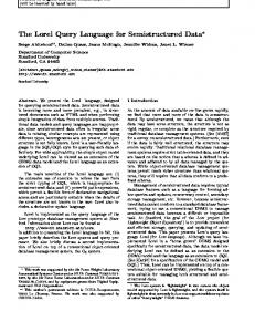
2. ORA-SS  the data model of our language The ORA-SS (Object-Relationship-Attribute model for Semi-Structured data) is a rich semantic data model for semistructured data. Besides reflecting the nested structure, it also distinguishes among object classes, relationship types and attributes in ORA-SS. Moreover, the ORA-SS specifies the participation constraints of object classes in relationship types and indicates whether an attribute belongs to an object class or a relationship type, which is the information lacked in OEM (Object Exchange Model) and DOM (Document Object Model). With the help of the semantic information in ORA-SS, we can develop a much powerful graphical query language for semistructured data. Before we discuss our query language, we give an introduction about ORA-SS. Suppose we have a DTD (named as “Department.dtd”) of the XML document “Department.xml” as Figure 1. The DTD in Figure 1 specifies the information about departments, courses and students. Every department has a unique name and provides one or many courses; every course has a unique course code, a title and one or many students; and every student has a unique student number, a grade under the course and his/her own name. The ORA-SS schema diagram of the DTD is in Figure 2. In ORA-SS, department, course and student are treated as object classes that are represented by labeled rectangles. The name of the department, course code and title, student number and name and the grade are treated as attributes under the corresponding object classes by using circles. The filled circles are the primary keys. The arrows indicate the nested structure of the schema and the labels on the edges are for relationship types. The label “2, 1:n, 1:1” near the arrow from department to course means: there is a binary relationship type between department and course; and one department can has one or many courses while one course can only belong to one department. The label “cs, 2, 1:n, 1:n” near the arrow from

department 2, 1:n, 1:1 course name

cs, 2, 1:n, 1:n student code

title number

cs name

grade

Figure 2. The ORA-SS schema diagram of “Department.dtd”

As a superset of DTD, the ORA-SS schema needs some semantic announcements from users [7]. Ignoring the labels on the edges, which are for relationship types, the ORA-SS schema diagram exactly reflects the nested structure of DTD. However, the labels of relationship types help us distinguish relationship type attributes from object class attributes. As a result, such kind of semantic information will aid us with view validation[6] in query processing.

3. Our graphical query language Our graphical query language, which we call GLASS (Graphical Query Language for Semi-Structured Data), is developed as a graphical language for users to extract information from semistructured data. The language should be able to express various queries clearly and concisely without ambiguity, and be simple to draw and easy to read. It should support aggregation functions, negation and other XQuery standards, which will be discussed in this paper. Other functionalities like data manipulation, control and integration will not be included in this paper. In this section, we firstly introduce the general ideas including the basic and advanced concepts in GLASS (in Section 3.1.1 and 3.1.2) and the output construction (3.1.3). Following that, we show how to express the basic queries such

as Selection, Projection (3.2.1) and Join (3.2.2). After that we present the aggregation functions (3.2.3) and the queries on order sensitive data (3.2.4). Finally, in Section 3.3, we give some complex query examples that are difficult to express in other graphical query languages.

3.1 General concepts in GLASS In GLASS, we use graphs to express user queries. Based on the ORA-SS model, most notations in GLASS are reused from the ORA-SS diagram. 3.1.1 Basic concepts (1) Data Icons: We basically have two data icons: rectangles and circles, which are the vertices in query graphs. (a) Rectangles represent the object classes in ORA-SS. If we map the rectangles into the XML schema, they are all nonterminal elements in XML (element with subelements or attributes). (b) Circles represent the attributes in ORA-SS, both object class attributes and relationship type attributes. When we match the circles into the XML schema, they are all terminal elements with PCDATA only and the attributes (or attribute lists) in XML. (2) Connections: Beside the icons, the connections in the query graphs also take important roles. (a) Arrow: the first connection is the arrows that are used to represent the relationships. (b) Dashed arrow: the dashed arrows are used to represent the IDREF in XML. Both types of arrows, the solid or dashed, are reused from ORA-SS diagram. (c) Line: the solid lines are used to specify constraints between outputs and original data in the query graphs. The line is not derived from ORA-SS, but XML-GL [4, 5], we will see the use of line in Query 7 (in Section 3.2.1.). (3) Box: The box is used to indicate group entities in our query graphs. The group entity consists of all rectangles or circles inside the box. In the query graph, a boxed group entity can be regarded as a complex vertex. The use of box will be mentioned in Section 3.3.1. 3.1.2 Advanced concepts (1) Derived entities: Derived entities, including derived object classes and attributes are represented as dashed rectangles and dashed circles. The dashed data icons are treated the same as solid ones in constructing outputs since they are the new data types defined by users (See Figure 9 in Section 3.2.3.) (2) Condition Logic Window (CLW): The condition logic window is an optional part in a GLASS

query. It is a place to write logic expressions and statements (e.g. IF-THEN) for complex query conditions rather than draw them in the graph. The use of CLW will be discussed in 3.3. (3) Path Identifier and Condition Identifier: Both identifiers are user-defined unique names of entities in query graphs. The entities here include all data icons, connections and boxes. The path identifiers are the unique names given to data icons or boxes. They start with “$” and are assigned at the right side of data icons or boxes between two “:”s. The path identifiers are used to represent the corresponding entities in query graph. The condition identifiers are the unique names given to the connections. They are assigned between two “:”s after the typename of the connection without beginning with “$”. The typename of the connection can be omitted when it is “default”. The condition identifiers stand for certain parts of query conditions. To both identifiers, the colons are not parts of the identifiers but distinguish them from the names of relationship types. (4) Logic Expression and Statement: Both logic expressions and statements are written in CLW. The statements are quoted by a pair of braces (“{}”) to be distinct from logic expressions. The logic expression specifies the logic over or among the conditions in query while the statement helps construct complex outputs. 3.1.3 Construct output Software Engineering John Smith A B Mel Green C A Database Design John Smith B

Figure 3. The content of “Department.xml”

One of the important features of XML data is the flexibility in its schema. One set of information can be organized in different ways according to different users. Therefore, we should allow user to define the needed output structure in GLASS. Recall the DTD file “Department.dtd” from Example 1 in Figure 1. The “Department.xml” in Figure 3 is supposed to be

the document according to the definition in “Department.dtd”. In Figure 4, we list series queries to construct different outputs and, based on the data in Figure 3, we compare the result in Figure 5. course

course

course

course

course @title

*

Query 2

Query 3

Query 4

Query 5

Software Engineering Database Design Query 2: Extract courses with all information at all levels under course elements by using the default output method

code

@ Query 1

course

Query 1: Extract courses with the information at one level under course elements by using the default output method

Query 6

Figure 4. Queries 1 to 6, the basic ways of output construction

Query 1. Extract courses and all information one level under course elements by using the default output method; Query 2. Extract courses and all information at all levels under course elements by using the default output method; Query 3. Extract courses with all attributes of course element in the original XML document; Query 4. Extract courses and all terminal entities at one level under course elements; Query 5. Extract courses and all entities (both terminal and nonterminal ones) at one level under course; Query 6. Extract courses with their titles as attributes and codes as subelements in the output. As we can see in Figure 5, by using the default output method, everything will be kept in the original style from source data as in Query 1 and Query 2. The wildcard “*” in Query 2 means all nested levels under course element. Query 3 extracts courses and all attributes of course elements in XML document. The symbol “@” near the circle implies all attributes of course element in the original XML document. Query 4 extracts courses and all terminal entities at one level under course elements. The so-called terminal entities are those leaf entities in the ORA-SS schema diagram. A terminal entity can be an attribute or a simple element with PCDATA only. The nonterminal entities are the elements with subelements or attributes in XML. Therefore, Query 4 only extracts course codes and titles. Query 5 uses a rectangle to extract the nonterminal entities one level under course elements such as “student”. Since we just extract the entities at one level under course, the student number at the second level under course doesn’t appear in the result. Also, the student elements appear NULL since they haven’t any contents except subelements and/or attributes. Query 6 is a demonstration of the conversion between attribute and subelement.

Software Engineering John Smith A B Mel Green C A Database Design John Smith B Query 3: Extract courses with all their attributes in the original XML document. Query 4: Extract courses with all terminal entities at one level under course elements Software Engineering Database Design Query 5: Extract courses with all entities at one level under course elements Software Engineering Database Design Query 6: Extract courses with their titles as attributes and codes as subelements in the output 201 303 1

Figure 5. The corresponding outputs of Queries 1 to 6

3.2 Basic query operators

3.2.1 Selection and projection

In this section, we present how we use GLASS to represent the basic query operators in most query languages: Selection, Projection and Join. Besides, the aggregation functions and the queries on order sensitive data will also be discussed.

Now we demonstrate how we express selection and projection in GLASS in comparison with XQuery. Query 7. FOR $c IN $department/course WHERE $c/@code/data() = ‘2%’ RETURN $c

The XQuery expression in Query 7 select all courses whose codes begin with “2”. In the XQuery expression, $c is a variable of element type “department/course” and “data()” is a keyword to extract data under the given path “$c/@code/”. We express the query as the graph in Figure 6. To project all courses with their titles, XQuery will give the following expression: Query 8. FOR $c IN $department/course RETURN { $c/title } This query will display all courses and extract their titles as subelements. In Figure 6, we draw this query as a simple construction. course

course

title description

ORA-SS schema diagram

Figure 7. The DTD and the ORA-SS schema diagram of “Description.xml” FROM Department.xml

course

FROM Description.xml course

code

course *

description

description

Figure 8. Query 11 in GLASS, join from two documents title

Query 7

code DTD

course

*

code =‘2%’

course



Query 8

Figure 6. Selection (Query 7) and Projection (Query 8) in GLASS.

The GLASS queries generally have two parts separated by a vertical line. The left hand side (LHS) is used to specify conditions, which is optional (See Query 8 where there is right hand side only.). In contrast, the right hand side (RHS) is used to define the output, which is compulsory. The solid line connecting two courses on both sides is a constraint that the courses in the result on the RHS are just the courses that satisfy the conditions on the LHS. In Query 7, the RHS has the same structure as Query 2 in Figure 4. Thus it will pick out all courses whose codes begin with “2” and extract all information of those courses in the same format as Query 2 does. 3.2.2 Join In this section we discuss the third basic query operation, join. Suppose we have another XML data named as “Description.xml” containing the descriptions of all courses; and the DTD and ORA-SS schema diagram (Figure 7) of “Description.xml” is shown as follows. Query 9. To extract everything of the courses from “Department.xml”, which have descriptions in “Description.xml”, and put the corresponding descriptions under the books in the results (See Figure 8). Notice that, in Figure 8, the line connects the course in the output with the course under “Department.xml” rather than “Description.xml”, which indicates that the extracted information about the courses comes from “Department.xml” as mentioned in Query 9. Thus, the result will contain the student information and grade as in “Department.xml”. Without this line or change the connection to the course under “Description.xml”, the query meaning and the result will also be changed. Similarly, the line connecting the description in the result

with the description under the course from “Description.xml” means that, in the result, the description elements come from “Description.xml”. Without this line, the description elements in the result will be NULL since the course in “Department.xml” doesn’t have a subelement called “description” 3.2.3 Aggregation functions course

course

_group student avg_grade

cs AVG grade

Figure 9. Query 10, aggregation function “average” over result

The GLASS also supports aggregation functions over results, such as “max”, “min”, “avg”, etc. Since the output value after aggregation process may not be the original data, we use derived data types to express the aggregation results. Query 10. For all courses, display courses with their information (in default way) and the average grade of each course (Figure 9). The “_group” label beside the arrows from course to student means: to group student under course. The element type “avg_grade” is a derived attribute in the results, which is the average grade of all students’ grades grouped under one course. The hexagon labeled as “AVG” is the aggregation function to get average value of grades of student grouped by course. 3.2.4 Query order sensitive data In XML, the data can be order sensitive. In ORA-SS, we express the order sensitive data by using the symbol “ 6 Query 13

Figure 13. Group with boxes (Query 12) and without boxes (Query 13)

In this section, we tend to introduce box and Condition Logic Window to express more complex queries. The queries are based on the data about projects, members and publications. The ORA-SS diagram of the data is shown in Figure 12. There are two relations in Figure 12. One is a binary relationship type between project and member and the other is a ternary relationship type among project, member and publication. For the binary relationship, one project can have one or many members and one member can attend one or many projects. As to the ternary relationship, one member in one project can write zero or many publications while one publication can belong to one or many (project, member) pairs.

In Query 12, the box is very important because it explicitly specifies the group entities. In contrast, Query 13, which has no box, makes a totally different meaning. Query 13. Display the members with names who have totally taken part in less than 5 projects and totally written more than 6 publications, and their names begin with character “S”. The first difference in Query 13 from Query 12 is that there is no box in the graph. The publication is grouped under member directly. However, to group publication under member in the ternary relationship among project, member and publication may cause duplicates in the results when a member has written one publication for two or more projects. Hence we use “CNT_UNIQUE” here, which is the second difference from Query 12, instead of “CNT” to eliminate duplicates in count.

3.3.1 Group entity

3.3.2 Negation

In GLASS, we use box to express group entity in query. Query 12. Display the members with names who have taken part in less than 5 projects but written more than 6 publications in some project they attended, and their names begin with the character “S” (Figure 13).

As mentioned in Section 3.1.2, we can use Condition Logic Window to express complex query conditions in GLASS. Here is an example of negation. Query 14. Display the members with their names who haven’t written any publication titled “Introduction to XML”.

number

title

Figure 12. The ORA-SS schema diagram of the data about “project, member and publication”

member

member

:A: publication name title = “Introduction to XML” CLW

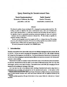
3.1.2, “$pro” is a path identifier. The prefix “$” distinguishes path identifiers from condition identifiers. Notice that the result of Query 15 will display the selected member in the original member order from the source data, and for those who have written “Introduction to XML”, the project information of them are also displayed.

4. Related works and comparison

¬∃ A;

Figure 14. Query 14, negation in query

In Query 14, “A” is a condition identifier, which stands for the condition that member has some publication titled as “Introduction to XML”. Then we put the logic expression “¬∃ A;” in CLW, which means “not exist condition A” in the selected member. Here, “∃” is the Existential quantifier and “¬” is the logic operator “NOT”. Other logic operators such as “∧” (and), “∨” (or) and “XOR” (disjunctive operator) as well as the universal quantifier “∀” are also available in GLASS. 3.3.3 IF-THEN Statement In some queries, the output may be conditionally organized such as “if some condition is satisfied, display the result in some way, otherwise, in some other way”. We express the statements in GLASS as follows. member

member :A: publication

:B: project : $pro :

publication name

title = “Introduction to XML”

title = “Introduction to Internet”

CLW A ∨ B; {IF (A) THEN EXTRACT $pro;}

Figure 15. Query 15, IF-THEN statement to construct complex output

Query 15. Display the members with their names who have written a publication titled “Introduction to XML” or “Introduction to Internet”; and for those members who have written “Introduction to XML”, also display all information about the projects that they have attended in (Figure 15). The part inside a pair of braces in the CLW is the IF-THEN statement that we use to express the query. Without this IFTHEN statement, the information of the projects of the members who have written “Introduction to XML” or “Introduction to Internet” will be displayed. The IF-THEN statement here secures that only when a member who has written “Introduction to XML” (i.e. when the condition “A” is satisfied), the information of the project of the member that is identified as “$pro” will be extracted. Recall from Section

When we talk about the graphical query language, QBE may be the first application that appears in our topic. As we mentioned in Section 1.2, QBE is both the language name and the system name of the early application by IBM in 1970s [9]. It is designed for relational database with table-like interfaces. QBE can express most SQL queries including selection, projection, join, aggregation and transitive closure. Along with the success of QBE, many graphical languages for relational data appear such as QBD* [2], GM (Graph Model) [3], GrIT [11] and Condor [14] etc. As to the semistructured data like XML, the graphical query languages for relational data cannot be simply modified even if we manage to store the data in an Object-Oriented and/or Relational Database Management System (OO/RDBMS) [1, 16] because there is no relation in XML schema and the XML documents are tree-structured data. Before we design the GLASS, there is only one graphical language designed for XML. Its name is XML-GL [4, 5], which shares some similarities with our GLASS. XML-GL is built on the base of a graphical representation of XML documents and DTDs, which is called XML graphs. XML graph represents the XML documents and DTDs by means of labeled graphs. All XML-GL queries consist of two parts, left hand side (LHS) and right hand side (RHS), which are similar to the Query 7 in Figure 6. The LHS of XML-GL indicates the data source and conditions, and the RHS constructs the output. The main difference between GLASS and XML-GL is the data model. GLASS uses ORA-SS data model that is a superset of DTD and XML Schema. The semantic information in ORASS secures the view validation; and the GLASS queries are view graphs constructed by the users as their wishes. However, based on the DTD or XML Schema, XML-GL has no mechanism to secure view validation. Thus, the LHS of XML-GL, which is the instance of the query, must keep the original data structure in XML graphs. Although users can construct the output, XMLGL doesn’t know whether the construction is valid or not. Compared with GLASS, XML-GL query graphs can be very sophisticated. XML-GL doesn’t indicate the group entities explicitly and has ambiguity in expression (especially when expressing IF-THEN statement in output construction). Other graphical XML query languages use nesting forms to express the nesting data structure in DTDs and/or XML Schema. Such applications as Graphical XML Query Language [13] and XMLApe Query Language [15] are exactly graphical user-

interfaces for users to query XML data. Users assign values into the forms to define the instances of queries. The first problem of these two graphical query languages is that neither of them support user-defined output construction. Besides, both use color to express join fields, which is not a good solution since some color can be very similar and the color only supports equijoin. The Table 1 compares our graphical query language with XML-GL, Graphical XML Query Language and XMLApe Query Language.

Data Model Selection, Projection and Join Query Order “Group by” operator and Aggregation function Negation Qualifiers (∀, ∃) Conditional output construction (e.g. IFTHEN clause) User-defined View View Validation

Graphical XMLApe XML Query [17] Language [15] XML XML DTD Schema

GLASS

XML-GL [4, 5]

ORA-SS

XML Graphs

Yes

Yes

Yes

Yes

Yes

Yes

No

No

Yes

Yes

No

No

Yes Yes

No No

No No

No No

Yes

No

No

No

Yes Yes

Yes No

No No

No No

Table 1. Comparison among GLASS, XML-GL, Graphical XML Query Language and XMLApe

5. Conclusion and future work GLASS (Graphical query Language for Semi-Structured data) is a powerful visual language to express queries on XML data. Based on ORA-SS, the GLASS creates a query environment of freedom, which allows user construct any view graphs that he thinks in the most natural way. GLASS combines the advantages of graphs and texts, which keeps the graphical part clear and makes the textual part easily understood. The future research work on GLASS is that: we firstly need to enhance the language, map the graphical expression into XQuery standard; then in the second step, we will expand the content of GLASS including data manipulation (e.g., INSERT, etc), data integration, and view maintenance to exploit the power of graphical method for querying XML data sources.

References [1] S. Abiteboul, D. Quass, J. McHugh, J. Widom and J. Wiener. The Lorel Query Language for Semistructured Data. Department of Computer Science, Stanford University. International Journal on Digital Libraries, 1(1):68-88, Apr. 1997. [2] M. Angelaccio, T. Catarci, and G. Santucci. QDB*: A graphical query language with recursion. IEEE Transactions on Software Engineering, 16(10):1150-1163, 1990. [3] T. Catarci, S.K. Chang, M.F. Costabile, S. Levialdi, and G. Santucci. A graph-based framework for multiparadigmatic visual access to databases. IEEE Transactions on Knowledge and Data Engineering,

8(3):455-475, 1996. [4] S. Ceri, S. Comai, E. Damiani, P, Fraternali, S. Paraboschi, and L. Tanca. XML-GL: a graphical language of querying and restructuring XML documents. In Proc. WWW8, Toronto, Canada, May 1999 [5] S. Ceri, S. Comai, E. Damiani, P. Fraternali, and L. Tanca. Complex Queries in XML-GL. SAC (2) 2000: 888-893 [6] Yabing Chen, Tok Wang Ling, Mong Li Lee: Designing Valid XML Views. To appear in the proceedings of 21st International Conference on Conceptual Modeling (ER'2002), October 7-11, 2002, Tampere, Finland. [7] Zhuo Chen. Extracting Schema from XML Documents. SoC, NUS. Honours Year Project Report. [8] Sara Comai, Ernesto Damiani, Letizia Tanca. The WG-Log System: Data Model and Semantics. INTERDATA technical report, T2-R06, July 1998. [9] C. J. Date. An Introduction to Database Systems. 3rd Edition, Addison-Wesley Publishing Company, 1981. [10] Gillian Dobbie, Wu Xiaoying, Tok Wang Ling, Mong Li Lee: ORA-SS: An Object-Relationship-Attribute Model for Semistructured Data. TR21/00, Technical Report, Department of Computer Science, National University of Singapore, December 2000. [11] P.W. Eklund, J. Leane, and C. Nowak. GrIT: An implementation of a graphical user interface for conceptual structures. Technical Report TR94-03, Computer Science Department, The University of Adelaide, February 1994. [12] Extensible Stylesheet Language (XSL) Specification. W3C Working Draft. Apr 1999. http://www.w3.org/TR/1999/WD-xsl19990421/ [13] Ankur Gupta, Zahid Khan. Graphical XML Query Language. Course paper. College of Computing, Georgia Institute of Technology, Sep 2000 [14] Joshua S. Hodas, Robert M. Keller, Ingo Muschenets, Jeffrey Polakow, Amy R. Ward and Will Ballard. Condor: A Simple, Expressive Graphical Database Query Language. Department of Computer Science, Harvey Mudd College. Computer Science Technical Report HMC-CS-97-04. [15] Leo Mark, etc. XMLApe. College of Computing, Georgia Institue of Technology. http://www.cc.gatech.edu/projects/XMLApe/ [16] Yuanying Mo, Tok Wang Ling. Storing and Maintaining Semistructured Data Efficiently in an Object-Relational Database. Research Report. SoC, NUS. [17] Jan Paredaens, Peter Peelman, Letizia Tanca. G-Log: A GraphBased Query Language. IEEE Transactions on Knowledge and Data Engineering, 7(3):436--453, June 1995. [18] Jayavel Shanmugasundaram, Kristin Tufte, Gang He, Chun Zhang, David DeWitt and Jeffrey Naughton. Relational Databases for Querying XML Documents: Limitations and Opportunities. VLDB 1999: 302-314 Department of Computer Sciences, University of Wisconsin-Madison. [19] XML Path Language (XPath) 2.0. W3C. Apr 2002. http://www.w3.org/TR/xpath20/ [20] XML Query Requirements. W3C. Feb 2001. http://www.w3.org/TR/xmlquery-req [21] XML Syntax for XQuery 1.0 (XQueryX). W3C. Jun 2001. http://www.w3.org/TR/xqueryx [22] XQuery 1.0 and XPath 2.0 Data Model. W3C. Apr 2002. http://www.w3.org/TR/query-datamodel/ [23] XQuery 1.0 and XPath 2.0 Functions and Operators Version 1.0. W3C. Apr 2002. http://www.w3.org/TR/xquery-operators/ [24] XQuery 1.0 Formal Semantics. W3C. Mar 2002. http://www.w3.org/TR/query-semantics/