GMDH METHOD WITH GENETIC SELECTION ALGORITHM ... - NNW

GMDH METHOD WITH GENETIC SELECTION ALGORITHM AND CLONING Marcel Jiˇrina∗, Marcel Jiˇrina jr†

Abstract: The GMDH MIA algorithm uses linear regression for adaptation. We show that Gauss-Markov conditions are not met here and thus estimations of network parameters are biased. To eliminate this we propose to use cloning of neuron parameters in the GMDH network with genetic selection and cloning (GMC GMDH) that can outperform other powerful methods. It is demonstrated on tasks from the Machine Learning Repository. Key words: Multivariate data, GMDH, linear regression, Gauss-Markov conditions, cloning, genetic selection, classification Received: July 14, 2009 Revised and accepted: September 17, 2013

1.

Introduction

Classification of multivariate data into two or more classes is an important problem of data processing in many different fields. For the classification of multivariate data into two classes the well-known GMDH MIA (group method data handling multilayer iterative algorithm) [1], [4], [5], [6], [7], [10], [20], [21] is often used. This approach – in contrast to others – can provide even a closed form polynomial solution [2]. Each neuron of the GMDH network has a quadratic transfer function of two input variables that has six parameters. The process of adaptation of the GMDH network is based on standard linear regression. However, it can be found that the mathematical conditions for linear regression [19] to get unbiased results are not fulfilled. It can be found that all neurons have slightly biased parameters and do not give an optimal solution. Here we introduce a cloning procedure for generating clones of a given neuron that may be better than the original “parent” neuron with the parameters stated ∗ Marcel Jiˇ rina Institute of Computer Science AS CR, Pod Vodarenskou vezi 2, 182 07 Prague 8 – Liben, Czech Republic, E-mail: [email protected], http://www.cs.cas.cz /∼jirina † Marcel Jiˇ rina jr Faculty of Information Technology, Czech Technical University in Prague, Th´ akurova 9, 160 00 Praha 6, Czech Republic, E-mail: [email protected]

c ⃝CTU FTS 2013

451

Neural Network World 5/13, 451-464

by linear regression. We show that cloning together with the use of genetic selection procedure leads to a new type of GMDH algorithm. We found that cloning is a simple and effective method for obtaining a less biased solution and faster convergence than that obtained by standard linear regression. At the same time, the use of genetic selection procedure allows all neurons already generated to remain potential parents for a new neuron. Thus the problem of deleting excessive neurons during learning disappears. We also discuss several causes for biased results of linear regression and show influence of heteroscedasticity too. Our results demonstrate that these influences can be easily eliminated by a simple cloning procedure and faster convergence and so better behavior of GMDH algorithm can be obtained. We suppose that our finding of causes for biased linear regression in the GMDH method and its solution by cloning may lead to finding other more effective procedures based e.g. on robust approaches.

2.

GMDH network

The standard GMDH MIA method has been described in many papers since 1971 e.g. in [1], [4], [5], [6], [7], [10], [20], [21]. The basis of the GMDH MIA is that each neuron in the network receives input from exactly two other neurons with the exception of neurons representing the input layer. The two inputs, x and y are then combined to produce a partial descriptor based on the simple quadratic transfer function (the output signal is z): z = a + b · x + c · y + d · x2 + e · y 2 + f · x · y where coefficients a, . . ., f are determined by linear regression and are unique for each neuron. The coefficients can be thought of as analogous to weights found in other types of neural networks. The network of transfer functions is constructed one layer at a time. The first network layer consists of the functions of each possible pair of n input variables (zero-th layer) resulting in n · (n−1)/2 neurons. The second layer is created using inputs from the first layer and so on. Due to the exponential growth of the number of neurons in a layer, after finishing the layer, a limited number of best neurons is selected and the other neurons are removed from the network. In the standard GMDH MIA algorithm all possible pairs of neurons from the preceding layer (or inputs when the first layer is formed) are taken as pairs of parents. The selection consists of selection of a limited number of the best descendants, “children”, while the others are removed after they have arisen and were evaluated. In this way all variants of GMDH MIA are rather ineffective as there are a lot of neurons generated, evaluated and then immediately removed with no other use. There are several works dealing with the genetic optimization of GMDH MIA method [7], [8], [9]. These approaches use GMDH networks of limited size as to the number of neurons in a layer and the number of layers. Some kind of randomization must be used to get a population of GMDH networks because the original GMDH MIA neural network is purely deterministic. Individuals in population are 452

Jiˇ rina M.: GMDH method with genetic selection algorithm and cloning

subjects of genetic operations of selection, crossover and mutation. As each GMDH network represents a rather general graph, there must be procedures for crossover of graphs similarly as in genetically optimized other kinds of neural networks, e.g., NNSU [10]. For example in [18] the NN architecture is built by adding hidden layers to the network, while configuration of each neuron connection is defined by means of GA. An elitist GA with binary encoding, fitness proportional selection, standard operators of crossover and mutation are used in the algorithm. Different genetically optimized GMDH networks in literature differ in the ways how a population, especially the first population of networks, is formed and by variants of genetic procedures used. It seems, however, that up to now no approach in genetically optimized GMDH networks has brought essentially better results than the standard GMDH MIA algorithm. On the other hand, genetically optimized GMDH networks eliminate the necessity to set up in advance at least the number of the best neurons left in each layer. In this way, such GMDH networks became even less “parameter-less” than before. The difficult problem with the genetically optimized GMDH method lies in the fact that a population of GMDH networks must be generated. There must be crossover of individuals. Individuals are networks, which generally have different graphs. The crossover of two different graphs is a rather complex task. Its solution is known and used also in other genetically optimized neural networks [10], [15], [16], [17].

3.

Linear regression

Usually – and we do it as well – the parameters of the new neuron are set up by linear regression, i.e. with a least mean squared error method. This method uses the following Gauss-Markov assumptions [19]: • The random errors have an expected value of 0. • The random errors are uncorrelated. • The random errors are homoscedastic, i.e., they all have the same variance. The errors are not assumed to be normally distributed, nor are they assumed to be independent, nor are they assumed to be identically distributed. We suspect that due to the nonlinearity of the problem as well as the GMDH network, the assumption of homoscedasticity is not met especially for the classification problem. In classification problems each class has a different origin from which a different distribution of regression errors may arise. We show here in an example that the Gauss-Markov assumptions of an expected value of 0 and of homoscedasticity need not be fulfilled in GMDH network. Therefore the solution obtained by the least mean squared error method need not be the optimal solution. The truly optimal solution may lie somewhere in the neighborhood of the solution found by the LMS method. Let us suppose the use of the GMDH network for a two-class classification problem, i.e. data samples belong to one or the other class. Two-class data are rather often in practice. For illustration we use breast cancer data from UCI 453

Neural Network World 5/13, 451-464

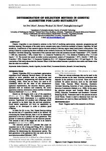
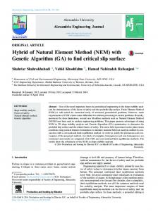
Machine Learning Repository [13]. Classes give a diagnosis, malignant (Class 0) or benign (Class 1). In Fig. 1 histograms of residuals, i.e. histograms of errors for one neuron and for both classes separately and for all data are depicted. There it can be seen that first, the expected value apparently is not zero, and second, residuals are heteroscedastic. The heteroscedasticity originates in the fact that there is data of two classes, each of different statistics. On the other hand, heteroscedasticity does not cause biased results per se. In only enlarges variation of estimate. The GMDH neuron is highly nonlinear and thus even signal with any symmetrical distribution is transformed so that resulting distribution is asymmetrical and results in biased mean after. Negative influence of the heteroscedasticity lies in larger variation and after nonlinear transformation in lager bias. It is shown in Fig. 2, where histograms of input signals to neuron analyzed are depicted.

Fig. 1 Histograms of residuals for both classes (Class 0 – malignant, Class 1 – benign) and for both classes together for the breast cancer data classification problem [13].

Fig. 2 Histograms of input signals for both classes (Class 0 – malignant, Class 1 – benign) and for both inputs of the neuron for the breast cancer data classification problem [13]. 454

Jiˇ rina M.: GMDH method with genetic selection algorithm and cloning

It can be seen that classes have very different statistics. After polynomial transformation according to (1) the difference increases because the target of the transformation is to get the output as close as possible to a value of 0 for class “malignant” and to a value of 1 for class “benign”. From this difference follows also the difference in the statistics of residuals – see Fig. 1 – after transformation (1) where coefficients were set up by linear regression. Different approaches can be used to find a better solution than the solution obtained by linear regression. The solution obtained by linear regression can be used as the first approximation. We use cloning, i.e. we generate neurons with the same inputs and with parameters a, . . ., f slightly modified with respect to their original values.

4.

GMDH with genetic selection

Here we describe the approaches which result in our construction of a genetically modified GMDH network with cloning. In fact, the network we propose is not genetically optimized in a standard sense as there is no population of GMDH networks and no crossing. The genetic selection and cloning regard the population of neurons of one GMDH network, not GMDH networks.

4.1

The learning set

We assume the n-dimensional real valued input and a one-dimensional real valued output. The learning set consists of n + 1 dimensional vectors (xi , yi ) = (x1i , x2i , . . . , xni , yi ), i = 1, 2, . . . , N where N is the number of learning samples (patterns or examples). The learning set can be written in the matrix form [X, Y ] . The matrix X has n columns and N rows; Y is a column vector of N elements. In the GMDH the learning set is usually divided into two disjoint subsets, the training set (or construction or setup set) and the so-called validation set. In the learning process the former one is used for setting up the parameters of neurons of the newly created neuron, the latter for the evaluation of an error of a newly created neuron. Thus N = Ns + NV , where Ns is the number of rows used for setting up the parameters of neurons (the training set), and NV is the number of rows used for error evaluation during learning (the validation set).

4.2

New genetically modified GMDH network algorithm

A very interesting and in principal simple application of selection process to GMDH MIA was published by Hiasaat and Mort in 2004 [8]. Their method does not remove any neuron during learning. Thus it allows unfit individuals from early layers to be incorporated at an advanced layer where they generate fitter solutions. Secondly, it also allows those unfit individuals to survive the selection process if their combinations with one or more of the other individuals produce new fit individuals, and thirdly, it allows more implicit non-linearity by allowing multi-layer 455

Neural Network World 5/13, 451-464

variable interaction. The GMDH algorithm is constructed in the same manner as the standard GMDH algorithm except for the selection process. In order to select the individuals that are allowed to pass to the next layer, all the outputs of the GMDH algorithm at the current layer are entered as inputs in the GP algorithm. It was shown in [8] that this approach can outperform the standard GMDH MIA when used in the prediction of two daily currency exchange rates. No other test of this approach classification ability was performed in the literature cited. The GMDH network [8] has a layered structure where input to the neuron can be output of any already existing layers or even network inputs. To keep a layered structure in this context seems rather complicated. One can use generalization where a new neuron input can be the output of any already existing neuron or even network input. Thus the strict layered structure disappears. An operation of a crossover in the GMDH with genetic selection is, in fact, no crossover in the sense of combining two parts of the parents’ genomes. In our approach eq. (1) gives a symmetrical procedure of mixing the parents’ influence but not their features, parameters. The parameters a, . . ., f , see (1), are stated separately.

4.3

Selection procedure

In genetic algorithms in the selection step there is a common approach that the probability of being a parent is proportional to the value of the fitness function. Just this approach is used here. The fitness is simply a reciprocal of the mean absolute error on the validation set. The initial state form n inputs only, there are no neurons. In this state two different inputs are selected randomly with equal probability as parents of a new neuron. If there are k neurons already, the probability of a selection from inputs (pi ) and from neuron outputs (pn ) is given by pi = n/(n + k), pn = k/(n + k) for n/(n + k) > p0 , where p0 is minimal probability that one of the network inputs will be selected as a parent of a new neuron; we found p0 = 0.1 as optimal. Otherwise, i.e. if n/(n + k) ≤ p0 pi = p0 , pn = (1 − p0 ). The probability that an input will be selected as a parent of a new neuron is then pi /n. The probability that an already existing neuron will be selected should be inversely proportional to the value of fitness function. The fitness function is equal to the reciprocal error on the verification set. Let ε(j) be the mean error of the j-th neuron on the validating set. The probability that neuron j will be selected is: 1/ε(j) . pn (j) = (1 − pi ) N ∑T 1/ε(s) s=1

456

Jiˇ rina M.: GMDH method with genetic selection algorithm and cloning

Technically, define first a number ri0 = 0, and then number ri1 = pi /n is assigned to the first network input, number ri2 = ri1 + pi /n is assigned to the second network input and so on until number rin = pi is assigned to the last network input. Then number rn1 = rin + pn (1) is assigned to the first neuron (j = 1), number rn2 = rn1 + pn (2) is assigned to the second neuron a and so on. After it a random number α between 0 and 1 with a uniform distribution is generated. If there is rik1 ≤ rik for some k then input k is selected as a parent. Similarly if there is rnk1 ≤ rnk then neuron k is selected as a parent. This is repeated once more for another random number to get two parents of a new neuron. Moreover, it must be assured that the same neuron or the same input is not selected as the second parent of the new neuron. After the new neuron is formed and evaluated it can immediately become a parent for another neuron. Thus the network has no explicit layers. Each new neuron can be connected to any input or already existing neuron. The computation of six parameters a, . . ., f , see (1), of the new neuron is the same as in the GMDH MIA algorithm. A new neuron added need not be better than all others. Therefore, the index and error value of the best neuron is stored until a better neuron arises. Thus every time there is information about the best neuron, i.e. the best network’s output without need of sorting. After learning, this output is used as a network output in the recall phase.

4.4

Cloning and mutation mechanism

From the ideas of artificial immune systems (AIS) [11] we use results of clonal selection theory, especially a cloning procedure derived from Simple Clonalg algorithm [12]. This procedure evaluates antibodies, randomly produces new antibodies, makes them maturate and lets the best of them survive. In biological systems, clones are not exact copies of the parent cell because some mutations are in effect. In the case of GMDH cloning, a similar idea is used. The GMDH cloning consists of two operations: an exact copy of a mother (parent) cell and a mutation that slightly modifies newly generated child cell. The actual cloning follows the main idea of the Simple Clonalg algorithm [12]. Cloning is made by copying the best neuron. Mutation is achieved such that to each parameter a, . . ., f a randomly generated value from normal distribution with zero mean and 1/6 of the original parameter’s value as a standard deviation is added. The original values of the parameters are thus slightly modified to fluctuate around the original values of respective parameters of the best neuron. The actual algorithm of cloning runs this way: BEGIN Let the Best GMDH Neuron with its parents (i.e. input signals from In 1 , In 2 ) and with six parameters a, b, ..., f is given REPEAT Make a copy of the Best Neuron. The clone keeps the same inputs In 1 and In 2 . Mutate parameters a, ..., f , i.e.

add a randomly chosen 457

Neural Network World 5/13, 451-464

value from normal distribution N(0,(parameter/6)2 ) to each respective original parameter’s value. Evaluate fitness of this clone neuron. If the clone behaves better than the Best Neuron, break this clone generating cycle and start this cloning algorithm from the beginning with the clone (the new Best Neuron again). UNTIL a terminal criterion is satisfied or the maximum number of clones is reached. END

4.5

Error development, and stopping rule

From the new strategy of network building in the GMC-GMDH method there also follows a stopping rule different from searching for minimal error on the validating set as in the original GMDH MIA method. In our case error on the validating set for the best neuron monotonously decreases having no minimum. On the other hand, the indexes of the best neurons became rather distant. For illustration see Figs. 4 and 5. The process can be stopped either when a very small change in error is reached, or too many new neurons are built without the appearance of a new best neuron or when a predefined number of neurons is depleted.

4.6

Pruning

After learning the best neuron and all its ancestors have their role in the network function. All others can be removed. Pruning reduces the size of the network graph to necessary neurons (nodes) and edges. In the end, the network has no clear layered structure like a network generated by the original GMDH MIA algorithm and most of the other GMDH algorithms including those genetically optimized.

4.7

Recall

After learning the resulting network is a feed-forward network. When a sample is applied to inputs, the outputs of individual neurons are computed successively according to their order numbers. Thus at any time all information needed for a neuron’s output computation is known. The last neuron is the best neuron and its output is the output of the whole network. If the network is used for approximation or prediction, the output only gives the approximation of the value desired. If the network is used as a two class classifier, one must set up proper threshold θ and the output value larger than or equal to this threshold means that the sample applied belongs to one class or it belongs to the other class. The value of threshold can be tuned with respect to classification error or to other features of the classifier. 458

Jiˇ rina M.: GMDH method with genetic selection algorithm and cloning

5.

Performance analysis

The classification ability of the genetically modified GMDH algorithm with cloning (GMC GMDH) was tested using real-life tasks from the UCI Machine Learning Repository [13]. We do not describe these tasks in detail here as all of them can be found in [13]. Main characteristics are summarized in Table 1. All the tasks are classification tasks to two classes with a different number of features and samples as well. These tasks serve as classification benchmarks for the proposed genetically modified GMDH algorithm. For each task the same approach to testing and evaluation was used as described in [13] for other methods. We also show the convergence of the learning process. Dimension (attributes, features) German 24 Adult 14 Brest CW 30 Shuttle-small 9 Spam 57 Splice 60 Vote 15 Data set

Classes

Total samples

2 2 2 2 2 3 2

1000 45222 424 5800 4601 3175 435

Learning set size 800 30162 212 3866 3064 900 300

Test set size 200 15060 212 1934 1537 100 135

Cross validation 1 1 1 1 1 10 1

Tab. I Characteristics of datasets used for evaluation of the classification ability of the GMC GMDH algorithm. The experiments described below show that our genetically modified GMDH algorithm with cloning (GMC GMDH) outperforms 1-NN method in most cases, in many cases outperforms na¨ıve Bayes method and also k-NN method where k equals to the square root of the number of training set points. For running the GMC GMDH program default parameters were used as follows for all tasks: No. of neurons generated for stopping computation was 10000. Probability that the new neuron’s input was one of the input signals was 10 %, probability that the new neuron’s input was one of the already existing neurons was 90 %. Maximal number of clones generated from one parent neuron was limited to int(sqrt(No. of neurons generated up to now)). For all methods optimal threshold θ for minimal error was used. Fitness function was the reciprocal of the mean absolute error. An experiment was done also with fitness function equal to the reciprocal of the square of the mean absolute error to make lower the relative probability that a bad neuron is selected as a parent for a new neuron. In Tab. II the results are shown together with the results for four other wellknown and very often used classification methods. In the second column the cross validation factor is given. The methods for comparison are 1-NN – standard nearest neighbor method Sqrt-NN – the k-NN method with k equal to the square root of the number of samples of the learning set 459

Neural Network World 5/13, 451-464

Bayes – the na¨ıve Bayes method using ten bins histograms LWM1 – the learning weighted metrics method [14] modified with nonsmooth learning process. These results are also depicted in digest form in Fig. 3.

Data set German Adult Brest CW Shuttle-small Spam Splice Vote

1-NN 0.4077 0.2083 0.0479 0.0259 0.0997 0.4035 0.1053

sqrt-NN 0.2028 0.2124 0.0326 0.0828 0.1127 0.3721 0.0602

Bayes 0.2977 0.1637 0.0524 0.1294 0.1427 0.2866 0.0977

Algorithm LWM1 GMC GMDH GMC GMDH 2 0.2814 0.2947 0.2617 0.1717 0.1592 0.1562 0.0454 0.0419 0.0436 0.0310 0.0259 0.0465 0.1074 0.1008 0.0917 0.2587 0.1309 0.1339 0.0741 0.0667 0.0741

Tab. II Classification errors calculated as a simple ratio of a number of misclassified cases to a total number of cases on the test set for four methods on some data sets from UCI MLR. GMC GMDH uses fitness function equal to the reciprocal of the mean absolute error, and GMC GMDH 2 uses fitness function equal to the reciprocal of the mean squared error.

Fig. 3 Classification errors for four methods on some data sets from the UCI MLR. Note that for Shuttle small data the errors are ten times enlarged in this graph. In legend GMC GMDH 2 means GMC GMDH method with fitness equal to the reciprocal of square of the mean absolute error. 460

Jiˇ rina M.: GMDH method with genetic selection algorithm and cloning

The learning process of the GMC GMDH network is stable and convergent. In Figs. 4 and 5 successive lowering of error is depicted. The error is stated on the validating set for data VOTE from UCI MLR. In contrast to the GMDH MIA algorithm there is no minimum and the stopping rule here is based on the exhausting of a total number of neurons given in advance.

Fig. 4 Error on the validating set count of best neurons successively found during learning.

Fig. 5 Error on the validating set vs. index of the best neuron, i.e. the number of neurons generated. 461

Neural Network World 5/13, 451-464

In Fig. 4 it is shown how an error of the best neuron on the validating set decreases with the number of best neurons successively found during learning. It is seen that in this figure the order number of the best neuron, i.e. the true number of neurons generated during the learning process is not seen. The dependence on the true number of neurons generated is shown in Fig. 5. There on the horizontal axis is the number of neurons generated and points on the line show individual best neurons successively generated. For each point the corresponding value on the horizontal axis is the order number of the best neuron.

6.

Discussion

It was found that our expectation was upheld, that the homoscedasticity condition is not fulfilled in the GMDH network and the true optimum may lie somewhere in the neighborhood of parameters computed by linear regression. Cloning is a useful technique to get closer to the true minimum. The cloning with large changes of parameters has little effect, but with small changes a new best neuron often arises. From it one can deduce that in practice differences between pairs of parameters corresponding to the minimum found by linear regression and the minimum found by cloning is not too large but not negligible. The new genetically modified GMDH method with cloning (GMC GMDH) has no tough layered structure. During learning when a new neuron is added it is connected to two already existing neurons or to network inputs randomly with some probability derived from fitness and keeping some minor probability that an input is selected. The fitness, i.e. the reciprocal of the mean absolute error is evaluated using the validating set. If a new neuron generated is found to be the best neuron the clones are derived to reach even better fitness. The clones have the same two “parent” signals as the best neuron. The mutation operation changes slightly the values of the six parameters of the best neuron and thus clones are similar to, but not exact copies of the best neuron. Classification errors also for four other methods on some data sets from the UCI MLR are depicted in Fig. 3. Note that for Shuttle small data the errors are ten times enlarged in this graph. In Tab. II and in Fig. 3 it is seen that the GMC GMDH method outperforms other methods in tasks Adult, Shuttle small, and Splice or nearly outperforms Brest CW, Spam, and Vote. The GMC GHMDH is the second best with very small differences with respect to the best method considered. It is the second best in task German. The experiments described above show that the GMC GMDH approach outperforms 1-NN method in most cases, in many cases outperforms na¨ıve Bayes method and also the k-NN method where k is equal to the square root of the number of training set samples. It is also seen here that for fitness function equal to the second power of mean absolute error, the error may be slightly different from the case of fitness function equal to mean absolute error. Then the sensitivity to fitness function definition is rather small in these cases. In Figs. 4 and 5 it is seen that the learning process converges rather fast, i.e. for the relatively small number of neurons generated the error on the validating set decreases fast and then for the large number of neurons generated the error only decreases slightly. Practical tests show that further enlargement of the number of 462

Jiˇ rina M.: GMDH method with genetic selection algorithm and cloning

neurons generated up to the order of hundreds of thousands has no practical effect. As there is no searching or sorting like in the nearest neighbor-based methods or in classical GMDH MIA algorithm, the GMC GMDH is much faster than methods mentioned especially for large learning sets. Here we have presented a new method of building the GMDH network with the genetic selection of parents for each new neuron and with cloning of the best neuron. We have shown efficiency and good behavior for two class classification tasks. As GMDH networks serve also as approximators and predictors the possibility is open to use GMC GMDH for approximating and predicting tasks in further research.

References [1] Ivakhnenko, A. G.: Polynomial Theory of Complex System. IEEE Trans. on Systems, Man and Cybernetics, Vol. SMC-1, No. 4, Oct. 1971, pp. 364-378. [2] Farlow, S. J.: Self-Organizing Methods in Modelling. GMDH Type Algorithms. Marcel Dekker, Inc., New York, 1984. [3] Tamura, H., Kondo, T.: Heuristics-free group method of data handling algorithm of generating optimal partial polynomials with application to air pollution prediction. Int. J. Systems Sci., 1980, vol. 11, No. 9, pp. 1095-1111. See also Farlow 1984 p. 225. [4] Ivakhnenko, A. G., M¨ uller, J. A.: Present State and New Problems of Further GMDH Development. SAMS, Vol. 20, 1995, pp. 3-16. [5] Ivakhnenko, A. G., Ivakhnenko, G. A., Mller, J.A.: Self-Organization of Neural Networks with Active Neurons. Pattern Recognition and Image Analysis, Vol. 4, No. 2, 1994, pp. 177-188. [6] Ivakhnenko, A. G., Wunsch, D., Ivakhnenko, G. A.: Inductive Sorting/out GMDH Algorithms with Polynomial Complexity for Active neurons of Neural network. IEEE 6/99, 1999, pp. 1169-1173. [7] Nariman-Zadeh, N. et al.: Modelling of Explosive Cutting process of Plates using GMDHtype neural network and Singular value Decomposition. Journ. of material processes technology, Vol. 128, 2002, No. 1-3, pp. 80-87. [8] Hiassat, M., Mort N.: An evolutionary method for term selection in the Group Method of Data Handling. Automatic Control & Systems Engineering, University of Sheffield, www.maths.leeds.ac.uk/statistics/ workshop/lasr2004/Proceedings/hiassat.pdf. [9] Oh, S. K., Pedrycz, W.: The Design of Self-organizing Polynomial Neural Networks. Information Sciences (Elsevier), Vol. 141, Apr. 2002, No. 3-4, pp. 237-258. [10] Hakl, F., Jirina, M., Richter-Was, E.: Hadronic tau’s identification using artificial neural network. ATLAS Physics Communication, ATL-COM-PHYS-2005-044, last revision: 26 August 2005, http://documents.cern.ch/cgi-bin/setlink?base=atlnot&categ=Communication&id=comphys-2005-044. [11] Ji, Z.: Negative Selection Algorithms: From the Thymus to V-Detector. Dissertation Presented for the Doctor of Philosophy Degree. The University of Memphis, August, 2006. [12] Guney K., Akdagli A., Babayigit B.: Shaped-beam pattern synthesis of linear antenna arrays with the use of a clonal selection algorithm. Neural Network world, Volume 16 (2006), pp. 489-501. [13] Bache, K., Lichman, M.: UCI Machine Learning Repository [http://archive.ics.uni.edu/ml]. Irvine, CA, University of California, School of Information and Computer Science, 2013. [14] Paredes, R., Vidal, E.: Learning Weighted Metrics to Minimize NearestNeighbor Classification Error. IEEE Transactions on Pattern Analysis and Machine Intelligence, Vol. 20, No. 7, July 2006, pp. 1100-1110.

463

Neural Network World 5/13, 451-464

[15] Zhang, M., Cieselski, V.: Using Bask propagation Algorithm and Genetic Algorithm to Train and refine neural networks for Object Detection. In: Bench-Capon T., Soda, G., Tjoa, A. M. (Eds.): Proceedings of 10th International Conference and Workshop on Database and Expert Systems Applications (DEXA 99), Lecture Notes in Computer Science, Vol. 1677, Springer, Heidelberg, 1999. [16] Chun Lu, Bingxue Shi: Hybrid back-propagation/genetic algorithm for multilayer feed forward neural networks. 5th International Conference on Signal Processing Proceedings, 2000. WCCC-ICSP 2000. (IEEE), Volume 1, 2000, pp. 571-574. [17] Kalous, R.: Evolutionary operators on ICodes. In: Proceedings of the IX PhD. Conference. Institute of Computer Science, Academy of Sciences of the Czech Republic, F. Hakl, Ed., Matfyzpress, Prague 2004, pp. 35-41. Held: Paseky nad Jizerou, Sept. 29 – Oct. 1, 2004. [18] Vasechkina, E. F., Yarin, V. D.: Evolving polynomial neural network by means of genetic algorithm: some application examples. Complexity International, Vol. 09, 2001, pp. 1-13. http://www.complexity.org.au/vol09/vasech01/ [19] Wikipedia – Gauss–Markov Markov theorem, 2009.

theorem

[online]

http://en.wikipedia.org/wiki/Gauss-

[20] Buryan, P.: Enhanced MIA GMDH algorithm. Proceedings of International Workshop on Inductive Modeling, 2007. ˇ [21] Kord´ık, P., N´ aplava, P., Snorek, M., Berezovskyj, G. M.: The Modified GMDH Method Applied to Model Complex Systems, In: International Conference on Inductive Modeling – ICIM 2002 (2002), pp. 150-155. http://link.springer.com/chapter/10.1007%2F978-3-64201530-4 6

464