GMProf: A Low-Overhead, Fine-Grained Profiling Approach for GPU

GMProf: A Low-Overhead, Fine-Grained Profiling Approach for GPU Programs Mai Zheng, Vignesh T. Ravi, Wenjing Ma*, Feng Qin, and Gagan Agrawal Dept. of Computer Science and Engineering, The Ohio State University 2015 Neil Avenue, Columubs, OH, USA {zhengm, raviv, qin, agrawal}@cse.ohio-state.edu

Abstract—Driven by the cost-effectiveness and the powerefficiency, GPUs are being increasingly used to accelerate computations in many domains. However, developing highly efficient GPU implementations requires a lot of expertise and effort. Thus, tool support for tuning GPU programs is urgently needed, and more specifically, low-overhead mechanisms for collecting finegrained runtime information are critically required. Unfortunately, profiling tools and mechanisms available today either collect very coarse-grained information, or have prohibitive overheads. This paper presents a low-overhead and fine-grained profiling technique developed specifically for GPUs, which we refer to as GMProf. GMProf uses two ideas to help reduce the overheads of collecting fine-grained information. The first idea involves exploiting a number of GPU architectural features to collect reasonably accurate information very efficiently, and the second idea is to use simple static analysis methods to reduce the overhead of runtime profiling. The specific implementation of GMProf we report in this paper focuses on shared memory usage. Particularly, we help programmers understand (1) which locations in shared memory are infrequently accessed? and (2) which data elements in device memory are frequently accessed? We have evaluated GMProf using six popular GPU kernels with different characteristics. Our experimental results show that GMProf, with all optimizations, incurs a moderate overhead, e.g., 1.36 times on average for shared memory profiling. Furthermore, for three of the six evaluated kernels, GMProf verified that shared memory is effectively used, and for the remaining three kernels, it not only helped accurately identify the inefficient use of shared memory, but also helped tune the implementations. The resulting tuned implementations had a speedup of 15.18 times on average.

I. I NTRODUCTION A. Motivation In recent years, Graphics Processing Units (GPUs) have become extremely cost and power effective and have garnered increasing popularity. Using a large number of simple, in-order cores, GPUs have been effective in scaling the performance of a variety of non-graphical applications across different domains, including financial modeling, weather forecast, computational biology, and many others [1], [2]. On one hand, GPUs are part of extreme-scale systems, e.g., in the list of top 500 supercomputers released in November 2011, three out of the top ten systems were built on GPUs [3]. On the other hand, commonly used desktops and laptops are having low or medium-end GPUs, which makes a highly parallel environment accessible and affordable to application developers who have no or little prior parallel programming experience.

*Pacific Northwest National Lab P.O.Box 999, Richland, WA, USA [email protected]

1. __global__ void transpose(float *odata, float *idata, int width, int height) 2. { … 3. __shared__ float shared_data[BLK_DIM][BLK_DIM]; 4. unsigned int xIndex = blockIdx.x * BLK_DIM + threadIdx.x; 5. unsigned int yIndex = blockIdx.y * BLK_DIM + threadIdx.y; 6. if ((xIndex < width) && (yIndex < height)) { 7. unsigned int index_in = yIndex * width + xIndex; 8. shared_data[threadIdx.y][threadIdx.x] = idata[index_in]; 9. }… 10. }

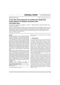
Fig. 1.

Sample code showing the use of shared memory.

Although CUDA [1] and subsequently OpenCL [4] have facilitated the trend of using GPUs for application acceleration, it remains very challenging to develop an efficient GPU implementation, especially for inexperienced developers. There are several reasons for this, including the need for careful management of GPU memory hierarchy, and similarly, the need for optimizing the execution of a large number of concurrent threads, while maintaining correctness. To promote wider use of GPUs, programmers need a variety of productivity and performance tools. The focus of this work is on such tools, and more specifically, on low-overhead yet accurate and fine-grained profiling methods. Particularly, we argue that fine-grained information is essential for optimizing a program on a modern GPU’s nuanced architecture. Meanwhile, unless a tool provides this information with a low or moderate overhead, it is unlikely that the programmers will use the tool. Unfortunately, existing profiling tools for GPUs [5]–[7] cannot provide sufficiently fine-grained information. Also, existing methods for profiling (typically developed for CPUs) either do not provide finegrained information [8]–[10], and/or will likely have prohibitive overheads [11] (if at all they can be implemented on a GPU). The main reason is that a very large number of threads are concurrently executed on a GPU, leading to a large number of concurrent events of interest (e.g., memory accesses), whereas the memory available for storing the information is very limited. B. Our Approach This paper presents a low-overhead and fine-grained profiling technique developed specifically for GPUs, which we refer to as GMProf. GMProf uses two ideas to help reduce the overheads of collecting fine-grained information. The first idea involves exploiting a number of GPU architectural features to collect reasonably accurate information very efficiently. The second idea is to use simple static analysis to reduce the overhead of runtime profiling.

The specific implementation of GMProf we report in this paper focuses on shared memory usage. Effective use of shared memory has been one of the most critical factors for application performance on GPUs. Figure 1 shows a simple GPU kernel that explicitly uses the shared memory, which is essentially a programmable cache. Line 3 declares and allocates the array shared data in shared memory and line 8 transfers data from device memory to the shared memory array. Developers need to maximize the utilization of this small yet extremely fast shared memory for achieving the best performance. This can be challenging, since it requires full knowledge on data use patterns, which are often unavailable at compile time. For example, memory addresses accessed at runtime may depend on the user input, or the executed control flow paths can vary at runtime. Various recent application studies on GPUs have demonstrated significant performance advantages from careful use of shared memory [12]. It should also be noted that while the latest NVIDIA cards do provide L1 and L2 cache, careful use of shared memory remains crucial for performance [13]. Thus, the implementation of the GMProf approach we present in this paper focuses on the following two critical questions: (1) which locations in shared memory are infrequently accessed? and (2) which data elements in device memory are frequently accessed? To answer these questions, the current implementation of GMProf includes two major components: Shared Memory Profiler and Device Memory Profiler. Given a GPU kernel, Shared Memory Profiler and Device Memory Profiler instrument the statements that access shared memory and device memory, respectively. At runtime, the instrumented code records the access numbers of shared memory and device memory into counter arrays. At the end of execution, GMProf processes the counter values and presents the summarized view of the results to developers for identifying inefficient use of memory. C. Summary of Contributions Overall, in this work, we have made the following contributions towards developing profiling tools for GPUs. Exploiting GPU’s Architecture: At program runtime, GMProf improves the performance by exploiting various GPU architectural features and properties of GPU programs. The observation underlying these optimizations is that developers are most interested in qualitative results (e.g., frequent or infrequent memory uses), instead of the very precise number of memory accesses. Specifically, the optimizations we perform include the use of faster (non-atomic) memory operations, storing information in smaller-sized counters in shared memory, and the use of threshold-based counter updates. While the last optimization reduces the number of counter update operations, the other two reduce the cost of each counter update operation. Combining Static Methods with Dynamic Methods: The second main observation in our work is that even for applications that cannot be completely analyzed at compiletime, simple compile-time information can significantly reduce runtime profiling costs. GMProf exploits simple static analysis to identify accessed memory addresses that are statically determinable, invariant to thread IDs, and/or invariant to loop iterators. The static analysis results help the dynamic profiling

components of GMProf eliminate, or reduce the number of memory accesses that need instrumentation. GMProf also leverages another static technique, i.e., live range analysis, to improve the accuracy of profiling in the case when multiple data elements are loaded into the same shared memory address during different phases of the program execution. Implementing, Evaluating, and Demonstrating a Prototype of GMProf: We have implemented a prototype of GMProf and evaluated it with six GPU kernel functions. We have shown that after various optimizations, the overheads of profiling are quite low for the evaluated kernels , i.e., 1.36 times for shared memory profiling and 55% for device memory profiling on average. Additionally, we have compared GMProf’s optimizations with a software sampling technique we implemented for GPU profiling. The results show that GMProf has a good balance of low runtime overhead and high accuracy comparing to sampling. Moreover, we have demonstrated the utility of the tool with three case studies. For each case, we show how the tool helps tune the application, and that the resulting optimized application has significantly better performance. II. R ELATED W ORK Our work is related to previous work on profiling tools and static analysis for memory hierarchy management. In both areas, we first focus on approaches specific to GPUs, and then summarize major efforts related to CPUs. Profiling Tools. GPU profiling tools include TAUcuda [5], NVIDIA Visual Profiler [6], and NVIDIA Parallel Nsight [7]. TAUcuda focuses on coarse-grained runtime events, whereas NVIDIA Visual Profiler and Parallel Nsight provide summarized information on GPU hardware counters (such as branch divergence#, launched warp#, non-coalesced device memory accesses). None of these tools can provide very fine-grained information, e.g., information that may help improve the use of shared memory. A recently proposed tool [14] profiles shared memory accesses to detect shared memory bank conflicts. However, this tool tracks every shared memory access in a brute force way, incurring prohibitive runtime overhead. Program optimization for memory hierarchy has been an important issue for uniprocessor (and multiprocessor) performance for at least the last two decades. Thus, CPU profiling tools have also focused on memory hierarchy related metrics. The relevant tools can be mainly classified into two categories: simulation-based (e.g., Cachegrind [11]) and hardware counter based approaches (e.g., Intel VTune [8], TAU [9] and Vampir [10]). Simulation-based approaches track each memory access. While these tools report cache misses at various granularity (e.g., thread, function, and source code lines), they incur prohibitive runtime overhead (e.g., Cachegrind slows down the programs by a factor of 20-100 times). On the other hand, by exploiting hardware performance counters and sampling techniques, the second category of tools [8]–[10] profile programs with much lower overhead. However, some of these approaches collect coarse-grained information [10], while others [8], [9] follow the techniques that are inapplicable to a programmable cache on GPU, which has to be explicitly managed.

Static Analysis Driven Approaches. Static analysis driven or compile time approaches for managing shared memory on GPU have been proposed by several researchers. Baskaran et al. developed data movement schemes for shared memory with a polyhedral model, targeting affine loops [15]. Udayakumaran et al. used a cost model based approach to allocate shared memory dynamically [16]. Ma et al. deployed an integer linear programming model to solve the problem of data arrangement on shared memory [17]. These approaches are either unable to deal with irregular and indirect accesses, or often in need of extra information such as the number of iterations in a loop. Compile time analysis for understanding cache reuse in CPUs has also been studied. Cascaval used stack histogram to analyze cache behavior [18]. Ding et al. proposed analysis algorithms to find data access patterns by using profiling [19], potentially providing intuitions for cache optimizations. Data reuse distance information is also used to exploit a new cache management scheme [20]. These approaches are not applicable when only a limited amount of information about control flow and/or data accesses is available at compile time. III. GMP ROF : D ESIRED F UNCTIONALITY AND C HALLENGES This section explains the challenges in profiling fine-grained information on a GPU, and especially, the space and time overheads as well as inaccuracy it can involve. As a specific example, we consider a trivial implementation of GMProf. Then, we list the challenges in collecting accurate profiling information efficiently. Consider the functionality of GMProf mentioned in Section I-B. Since the shared memory is explicitly allocated by a programmer, each memory access instruction either accesses a shared memory location or a device memory location. Therefore, profilers for shared memory and device memory are two independent components of GMProf. We discuss simple implementations of each of them next, and highlight the time and space efficiency issues. A. Profiling Shared Memory Use Shared Memory Profiler needs to track accesses for each shared memory address. Specifically, given that the size of the shared memory is very small (e.g., 16 KB on Tesla C1060 and at most 48 KB on recent Fermi cards), the profiler can maintain one counter for each shared memory address. Whenever a shared memory access occurs, the profiler can increase the corresponding counter value by one. It can use integer (32-bit) counters to accommodate potentially large numbers of memory accesses. Once the access number reaches the maximum value (i.e., 232 − 1), the profiler can stop increasing the counter. Another problem in obtaining correct counts is that different threads in a GPU kernel may access (read or write) the same shared memory address concurrently, leading to race conditions when updating the corresponding counter. To address this issue, Shared Memory Profiler can use atomic operations that are supported in CUDA and OpenCL. The above simple design clearly involves high space and time overheads. Since typical GPU kernels perform computations on four-byte (or eight-byte) data types, such as integer, float, or double, the profiler needs to keep one counter for

every four bytes in shared memory. This means that, in the worst case, the profiler needs the memory space with the same size as that of shared memory. On the other hand, the required space is a small fraction of the size of device memory, so we can expect to store these counters on device memory with relative ease. However, this can lead to a very high runtime overhead. For each shared memory access, the profiler introduces an atomic operation on device memory, which can be more than 100 times slower than a shared memory access. B. Profiling Device Memory Use Unlike Shared Memory Profiler, Device Memory Profiler cannot track the use of the entire device memory due to its huge size (e.g., 4 GB for Tesla C1060 cards). Furthermore, tracking the use of the entire device memory may not be a cost-effective way since many GPU kernels do not use up the entire memory. Therefore, Device Memory Profiler should track device memory space that have been used by the GPU programs. More specifically, for each declared device memory array, Device Memory Profiler can create a shadow array for counters, where each element (32-bit) in the shadow array stores the access number of the corresponding element (32-bit or 64-bit) in the tracked device memory array. For each device memory access, the profiler can increase the corresponding counter. Similar to Shared Memory Profiler, Device Memory Profiler can store the shadow arrays in device memory and uses atomic operations for updating the counters. As a result, in this simple design, the profiler adds one device memory atomic operation for each access to device memory. This itself can be a substantial overhead, since an atomic operation on device memory is much slower than a normal read or write on device memory. C. Design Challenges Challenge 1: Profiling Efficiency. Our discussion above has clearly pointed to challenges in time and space efficiency when profiling. Particularly, to leverage massive parallelism for best performance, GPU kernels typically launch hundreds or thousands of concurrent threads. Each thread, in turn, issues a memory access operation every few cycles. In trying to obtain efficiency, we must pay attention to the cost of different operations on GPUs. For example, the cost of each device memory access is much higher than a shared memory access, and atomic operations are significantly more expensive than the non-atomic operations. Section IV presents how GMProf addresses this challenge. Challenge 2: Profiling Accuracy. There is another challenge in obtaining accurate information of shared memory use. A simple scheme is to tabulate the aggregate number of accesses to each shared memory address. However, it will only work for GPU kernels that perform a simple memory management, i.e., where a chunk of shared memory is dedicated for a certain piece of data throughout the kernel execution. For longer running kernels, it is often desirable that a section of shared memory holds different data at different periods during the execution. A simple address-based scheme will not provide accurate information for such programs. Section V presents how GMProf addresses this challenge.

Two well-studied approaches can be used for optimizing a program’s use of memory hierarchy, while reducing or eliminating the overheads of profiling. The first mechanism is collecting data via sampling [21]–[26]. For comparison purpose, we have designed and implemented a GPU-specific sampling scheme that appeared most appropriate for addressing our problem. More details are discussed in Section VI-B. The second approach involves the use of static analysis and can completely eliminate any runtime costs [15], [27]– [30]. However, static analysis is applicable only if both of the memory addresses and the number of accesses are statically determinable. Unfortunately, this is not the case for many scientific, computation-intensive applications that are suitable for GPUs. In fact, a recent study has shown that many GPU kernel functions have dynamic irregularities in both memory references and control flows [31]. IV. GMP ROF : E FFICIENT P ROFILING A PPROACH We now describe the optimized profiling approach for GPU architectures that we have developed. This section specifically focuses on runtime overhead reducing mechanisms we have introduced. As we stated earlier, our approach involves use of simple static analysis, GPU architectural features, features of GPU programs, and an understanding of how profiling information is likely to be used by application developers, to reduce profiling overhead. A. Static Analysis (SA) Optimization As we stated earlier, profilers are most useful for applications where all accesses and execution paths cannot be resolved at compile time. However, even in dynamic or irregular applications, many memory accesses can be resolved statically. The SA optimization we introduce reduces the number of counter update operations for both Shared Memory Profiler and Device Memory Profiler. The first step involves scanning all memory references in a GPU kernel and checking whether the addresses as well as the corresponding access numbers can be resolved at compile time. If so, GMProf does not need to monitor such memory accesses at runtime. In the next step, SA checks whether a memory reference is dependent on thread IDs (e.g., threadIdx.x). If not, such memory access is invariant to thread IDs (referred to as tid-invariant), i.e., different threads access the same memory address. This information is annotated and passed to the profilers (i.e., Shared Memory Profiler and Device Memory Profiler) for optimized profiling. At runtime, we use a single thread to add the total number of threads, which can be obtained from the kernel configuration, to the corresponding profiling counter. In this way, we keep the correct counts while avoiding the contention of counter updates from hundreds or thousands of threads completely. More importantly, this step makes another optimization (NonAtomic Operations) possible (discussed in Section IV-B). Finally, SA checks each array index within a loop or a nested loop to see whether the index is dependent on loop iterators. If not, such memory access is invariant to loop iterators (referred to as loop-invariant). This information is annotated and passed to the profilers for optimized profiling.

1. __device__ void RClusterCnt (float *data, int nRowCL, int *colCL, …) 2. { … //Computation and reduction on memory 3. for (int r = 0; r < nRow; r+= ROWCL_THRDS * ROWCL_BLKS ) { 4. for (int rc = 0; rc < nRowCL; rc ++) 5. if (rowCS[rc] > 0) 6. for (int c = 0; c < nCol; c++) { 7. tempDistance += data[(r + n_idx) * nCol + c] * Acomp[rc * nRowCL + colCL[c]]; 8. …} 9. …} 10. }

Fig. 2.

Simplified code of Co-clustering kernel.

For a loop-invariant, since the number of accesses is determined by the number of iterations, the profilers do not need to update the counter in every iteration. Instead, the profilers only instrument the last iteration by performing one-time counter update operation, i.e., adding the number of iterations (determined at runtime) to the corresponding counter. Note that we perform the standard conservative static analysis here. We consider an access to be loop-invariant only if: 1) its value does not change across iterations of the loop, and 2) it is accessed in every iteration of the loop (i.e., it is not enclosed in a conditional statement). In cases where certain part of the code or the context cannot be analyzed, e.g., if there are procedure calls involved, SA optimization will not report the expression as being loop-invariant, and the memory access is monitored during runtime. To explain how static analysis optimization works, we take the simplified Co-clustering kernel in Figure 2 as an example. This kernel contains the aforementioned memory accesses that are tid-invariant or loop-invariant. For example, the access to rowCS (line 5) is independent of the outermost loop iterator r, which means it is r-loop-invariant access. In addition, it is independent of thread IDs and thus is also identified as tidinvariant access. B. Non-Atomic Operation (NA) Optimization As we described in the previous section, our initial approach for profiling involved the use of atomic operations, to avoid race conditions when concurrent threads access the same location. These operations turn out to be quite expensive especially when the number of competing threads is large. Thus, we introduce NA optimization, where we replace atomic operations with the normal (non-atomic) operations for updating counter values. This optimization can improve the efficiency of each counter update operation. At the first glance, however, it appears that this optimization may significantly compromise the accuracy of the access counts we obtain. Specifically, in the case when all threads access the same memory location at the same time, the access count obtained with non-atomic operations may be very small. However, with the help of the SA optimization discussed earlier, it turns out that such inaccuracy can be avoided to a great extent. Specifically, static analysis can help identify threadinvariant memory accesses, and consolidate concurrent updates of the same counter. As shown in our experimental results, after applying the SA optimization, the use of non-atomic operations does not impact the overall accuracy in almost all of the cases.

C. Shared Memory Counters (SM) Optimization The next optimization we introduce reduces the runtime overhead of shared memory profiling further. Specifically, it maintains the counters for Shared Memory Profiler in shared memory instead of device memory. The rationale is that device memory has much higher latency than shared memory (e.g., 150 times slower on Tesla cards), and therefore updating counters in shared memory for Shared Memory Profiler can significantly reduce the cost of each counter update operation. The basic SM optimization stores 32-bit profiling counters in shared memory instead of device memory. However, since the size of shared memory is very limited, the 32-bit counters can not fit in shared memory without incurring large space overhead. Thus, the basic SM optimization may not be applicable for all applications. On the other hand, to qualitatively identify frequent or infrequent use of shared memory, it might be unnecessary to maintain a 32-bit counter to keep counting to a large number. Based on this observation, we can use less bits for storing a profiling counter, For example, a configuration of 16-bit counters reduces half of the required space, while a 8-bit configuration reduces 75% space overhead. As a result, the SM optimization can be applied to more applications. With a small-sized counter, however, the counting could exceed the maximum value and lead to wrong results. The next optimization avoid such a overflow problem and make the SM optimization safe and more applicable. D. Threshold (TH) Optimization As we discussed earlier, one main problem with the trivial approach for collecting profile information is the number of updates performed on the counters, and the space required for the counters. We make the observation that programmers are most interested in qualitative information, as opposed to precise access counts. For example, a programmer would like to know whether a memory address is frequently accessed or not. Thus, while the difference between, say, 10 accesses and 1000 accesses may be important, difference between 1000 and 1010 accesses may not be in certain cases. Thus, we propose TH optimization, where we maintain counts up to a predefined threshold, i.e., stop updating the counters once the values reach a certain threshold. In this way, we reduce the number of counter update operations, which, in a memory bandwidth limited GPU, are extremely expensive. As shown in Section VI, it turns out that this idea can further lower the profiling costs on GPUs even after applying the previous three optimizations. Moreover, as mentioned in the previous section, use of thresholds also enables use of fewer bits for maintaining counters, which also has substantial benefits such as make the SM optimization more applicable. To implement the TH optimization, GMProf adds a threshold as the upper bound of the counter values. The profilers check the value of a counter before it is updated, and increase the counter only if the value is below the threshold. In essence, the TH optimization is a tradeoff between overhead and accuracy. A smaller threshold value incurs lower runtime overhead since fewer updating operations are performed. On the other hand, a larger threshold value provides more accurate memory use information to developers. The appropriate thresholds for

Algorithm 1 Optimized Shared Memory Profiling 1: if shared memory is available then 2: Create dynamic count array in shared memory 3: else 4: Create dynamic count array in device memory 5: end if 6: for each shared memory access do 7: if isStaticDeterminable(shm addr) and isStaticDeterminable(access count) then 8: static count[shm addr] = access count 9: else if isLoopInvariant(shm addr, iterator) then 10: if (! isStaticDeterminable(n iter)) then 11: Compute n iter 12: end if 13: if isLastIteration(iterator) then 14: if isTidInvariant(shm addr) and (tid == 0) then 15: inc = n iter * N T HREADS 16: dynamic count[shm addr] = min(dynamic count[shm addr] + inc, T HRESHOLD) 17: else 18: dynamic count[shm addr] = min(dynamic count[shm addr] + n iter, T HRESHOLD) 19: end if 20: end if 21: else if isTidInvariant(shm addr) and (tid == 0) then 22: dynamic count[shm addr] = min(dynamic count[shm addr]+N T HREADS, T HRESHOLD) 23: else if dynamic count[shm addr] ¡ T HRESHOLD then 24: ++ dynamic count[shm addr]; 25: end if 26: end for

different GPU applications are tunable and can be specified by developers based on prior program executions. For example, if multiple frequently-used memory addresses need to be differentiated (e.g., all of their access numbers are above the threshold), developers can increase the threshold based on prior runs and profile the program again until reaching the desired results. E. Overall Profiling Algorithm We now show how our runtime optimizations and the information from the SA optimization are integrated. Algorithm 1 shows the algorithm for Shared Memory Profiler with all the optimizations enabled. Specifically, the profiler creates a counter array in shared memory for every shared memory address. In the case of insufficient shared memory, the counter array is created in device memory instead (lines 1-5). The SA optimization provides three types of information for guiding instrumentation, i.e., statically determinable references (lines 7-8), loop-invariants (lines 9-20), and tid-invariants (lines 1416 and 21-22). For statically determinable references, the

counts are recorded at compile time (line 8). For loopinvariants, the number of iterations (n iter) is computed at run-time (line 11) if it is not statically determinable. The counter is incremented only in the last iteration (lines 13-20). If the access is tid-invariant as well, the increment (inc) is the multiplication of the number of iterations and the number of threads, and only one thread (tid == 0) is used to perform the update (lines 14-16). Otherwise, all threads increase their corresponding counters by the number of iterations (lines 1718). For tid-invariants that are not loop-invariants, one thread is used to increase the counter by the number of threads (lines 2122). Note that a threshold code (T HRESHOLD) is checked when updating counters to guarantee that the counts do not exceed the threshold (lines 16, 18, 22, 23). Also, the NA optimization, which is using non-atomic operations to update counters, is used at the relevant statements (lines 16, 18, 22, 24) in this algorithm. The algorithm for Device Memory Profiler is similar to Algorithm 1 except that the SM optimization is inapplicable. V. E NHANCED A LGORITHM : I MPROVING P ROFILING ACCURACY This section presents an enhanced profiling algorithm, which addresses an important limitation of Algorithm 1. Particularly, the methods we have presented so far cannot handle the situation when a shared memory address holds different data elements during different periods of a kernel’s execution. In such a case, the number of accesses to a shared memory address reported by Algorithm 1 may not directly reflect the frequency of data use, and can only mislead developers. To understand the limitations of the techniques presented so far, consider the following example. A GPU kernel first loads an array section S1 from device memory to shared memory, performs some simple computation while reading data from the shared memory array only once, and then stores the results back to device memory. Next, the kernel loads the array section S2 to the same shared memory location, for a similar computation and stores the results back to device memory. Suppose this process repeats for many different array sections. In this scenario, the shared memory addresses involved do not have any data reuse, and the shared memory is not being effectively used. However, Algorithm 1 will report a relatively high number of accesses to these shared memory addresses, and thus mislead the application developers in believing that data stored in shared memory has a high reuse. To overcome the above-memtioned limitation, we introduce an enhanced profiling algorithm based on dynamically computed live ranges [32]. For our purpose, the live range of an array section originally stored in a device memory location is defined as the interval between the time when the data is loaded from the device memory location to a shared memory location and the time when the data (which may be overwritten by intermediate computation results) is stored back from the same shared memory location to the same or different device memory location. Our enhanced profiling algorithm uses the live range information to accurately track the access numbers for each piece of device memory data during its live range in shared memory.

In the enhanced algorithm, the Shared Memory Profiler maintains a logical clock, which monotonically increases and marks the boundary of live range for each data. Furthermore, the Shared Memory Profiler creates a shadow array of counters in shared memory for each shared memory array declared in a GPU kernel. For each statement that loads data from device memory to a shared memory array (i.e., the beginning of a live range), the profiler increases the logical clock by one, resets the corresponding shadow array counters, and records the logical clock value to the shadow array. Within the data live range, the shadow array of counters are updated using Algorithm 1. For each statement that stores data from a shared memory array to device memory (i.e., the end of a live range), the profiler increases the logical clock by one and stores the values in the corresponding shadow array of counters into device memory. Additionally, the profiler stores the logical clocks for the live range and the shared memory array name with the shadow array of counters for this live range. Note that this algorithm maintains one global logic clock, and only one thread is needed for updating the clock. Also, while the live ranges are computed dynamically, static analysis helps identify all the statements that transfer (i.e., load or store) data between device memory and shared memory. Due to space limit, the formal description of the algorithm is omitted. Please refer to our technical report [33] for more details. VI. E XPERIMENTAL R ESULTS We have conducted the experiments using a NVIDIA Tesla C1060 GPU with 240 cores (8 cores/streaming multiprocessor * 30 streaming multiprocessors), a clock frequency of 1.296 GHz, 16 KB shared memory per streaming multiprocessor, and 4 GB device memory. This GPU was connected to a machine with two AMD 2.6 GHz dual-core Opteron CPUs and 8 GB main memory. We have implemented the prototype of GMProf based on CUDA Toolkit 3.0. Note that we do not see any particular difficulty to port GMProf to other GPU environments such as OpenCL [4] or stream SDK [34]. We have evaluated GMProf with six applications, including Co-clustering (referred to as co), EM clustering (referred to as em), Binomial Options (referred to as bo), Jacobi (referred to as jcb), Sparse Matrix-Vector Multiplication (referred to as spmv), and DXTC (referred to as dxtc). Among these applications, both co and em are data mining algorithms, bo is a financial modeling algorithm, jcb and spmv are stencil computation applications, and dxtc is a texture compression algorithm. We show the efficiency and accuracy of GMProf in this section. Additionally, we demonstrate the effectiveness of GMProf in the next section. Due to space limit, the space overhead is discussed briefly in VI-C and VII-B. Please refer to our technical report [33] for details. A. Runtime Overhead The current implementation of GMProf can be used for profiling shared memory use only, or for profiling device memory use only, or profiling both. A programmer who is interested in examining whether their implementation is adequately using shared memory is likely to profile shared memory only, whereas a programmer who is interested in examining what arrays from device memory should be allocated

Apps Native co 39.50 em 129.57 bo 16.59 jcb 163.31 spmv 21.25 dxtc 21.94 Average

GMProf-basic 7186.75 (180.93x) 18738.61 (143.62x) 1503.53 (89.63x) 951.07 (4.82x) 381.52 (16.95x) 14229.70 (647.57x) 180.59x

GMProf-SA 55.98 (0.42x) 131.54 (0.02x) 122.59 (6.39x) 951.07 (4.82x) 341.06 (15.05x) 14229.70 (647.57x) 112.38x

GMProf-SA-NA 72.27 (0.83x) 131.00 (0.01x) 35.35 (1.13x) 560.06 (2.43x) 70.34 (2.31x) 338.20 (14.41x) 3.52x

GMProf-SA-NA-SM 46.96 (0.19x) 131.00 (0.01x)* 30.20 (0.82x) 560.06 (2.43x)* 40.72 (0.92x) 132.36 (5.03x) 1.57x

TABLE I RUNTIME OVERHEAD OF DIFFERENT SCHEMES FOR PROFILING SHARED MEMORY USE . N ATIVE MEANS RUNNING A GPU KERNEL WITHOUT ANY PROFILING . GMP ROF - BASIC MEANS RUNNING A GPU KERNEL WITH THE TRIVIAL DESIGN OF GMP ROF . GMP ROF -SA IS APPLYING THE SA OPTIMIZATION TO GMP ROF - BASIC . NA MEANS APPLYING THE NA OPTIMIZATION , AND SM MEANS APPLYING THE SM OPTIMIZATION . I N EACH CELL OF THE TABLE , THE FIRST NUMBER IS THE EXECUTION TIME OF A GPU KERNEL IN MILLISECONDS AND THE SECOND NUMBER WITHIN A PARENTHESIS IS THE RUNTIME OVERHEAD COMPARED TO THE NATIVE EXECUTION . T HE LAST ROW SHOWS THE ARITHMETIC AVERAGE OVERHEAD OF DIFFERENT SCHEMES . * U SE DEVICE MEMORY DUE TO INSUFFICIENT SHARED MEMORY FOR SM OPTIMIZATION .

in shared memory may profile device memory only. Thus, we have conducted two separate sets of experiments to measure the overheads incurred by GMProf’s Shared Memory Profiler and Device Memory Profiler, respectively. 1) Runtime Overhead for Shared Memory Profiling: To measure the efficiency of shared memory profiling and the performance contribution of the different optimizations, we run each GPU kernel in five configurations, including (1) Native: the native run without any profiling instrumentation, (2) GMProf-basic: the run with the trivial scheme (i.e., no optimizations) of shared memory profiling, (3) GMProf-SA: the run with GMProf-basic and the SA optimization applied, (4) GMProf-SA-NA: the run with GMProf-basic and the SA and NA optimizations applied, and (5) GMProf-SA-NASM: the run with GMProf-basic and the SA, NA, and SM optimizations applied. Table I shows the execution time and runtime overhead (within the parentheses) for the six GPU kernels in all the configurations. As for TH optimization, we evaluate it separately in section VI-C since it represents an adjustable tradeoff between overhead and accuracy. Table I demonstrates that the trivial profiling scheme (GMProf-basic) incurs very large runtime overhead. For example, GMProf-basic adds 647.57 times overhead for dxtc. The main reasons for the prohibitive runtime overhead are that the device memory has a high latency, the atomic operations are time-consuming, and the number of tracked memory accesses is huge. Therefore, the trivial profiling scheme is impractical for profiling the memory use of GPU programs. After enabling the three optimizations, GMProf incurs a low to modest overhead for all six GPU kernels. As shown in Table I, GMProf adds 19%-5.03 times with an average of 1.57 times runtime overhead to the native run of the GPU kernels. As an example, by applying the three optimizations, GMProf reduces the overhead for bo from 89.63 times to 82%. This is because GMProf exploits GPU architecture-conscious optimizations and leverages invariant information provided by simple static analysis for reducing the number of counter update operations and improving the efficiency of each counter update operation. With the modest overhead, we found that GMProf is well suited for performance debugging or tuning. Furthermore, different optimizations improve GMProf’s efficiency for different GPU kernels to different extent, depending upon the nature of the application. For example, the SA optimization reduces the overhead incurred by GMProfbasic by orders of magnitude for co, em and bo, while reduces little for the others. This is because the effect of

Apps

Native

co

39.50

em

129.57

bo

16.59

jcb

163.31

spmv

21.25

dxtc

21.94

Average

GMProf -basic 3,304.29 (82.64x) 25,563.46 (196.29x) 52.76 (2.18x) 542.74 (2.32x) 45.63 (1.15x) 30.71 (0.40x) 47.50x

GMProf -SA 155.00 (2.92x) 260.79 (1.01x) 19.00 (0.15x) 542.74 (2.32x) 45.05 (1.12x) 30.71 (0.40x) 1.32x

GMProf -SA-NA 61.13 (0.55x) 151.38 (0.17x) 18.95 (0.14x) 491.71 (2.01x) 36.12 (0.70x) 22.04 (0.01x) 0.60x

TABLE II RUNTIME OVERHEAD OF DIFFERENT SCHEMES FOR PROFILING DEVICE MEMORY USE . T HE FOUR CONFIGURATIONS AND RESULTS HAVE THE SAME MEANINGS AS THOSE IN TABLE I. N OTE THAT THE SM OPTIMIZATION DOES NOT APPLY HERE .

SA optimization depends on the number of memory accesses that can be determined completely at compile time, as well as the number of loop-invariant and tid-invariant memory accesses that can be identified in the GPU kernel. For co, em and bo, the SA optimization significantly reduces the number of counter update operations, which can also alleviate contention from these counter update operations from a large number of concurrent threads. The NA and SM optimizations further reduce the overhead incurred by GMProf-SA through improving the efficiency of each counter update operation. Note that for em and jcb, the SM optimization is inapplicable since there are insufficient free shared memory. As we will see in section VI-C, by adding TH optimization, the SM optimization can be applied to the two applications. One exception for the effectiveness of the NA optimization occurs in co, where the NA optimization even adds overhead to GMProf-SA. In co, after applying the SA optimization to GMProf-basic, only one thread needs to update the profiling counter for a frequently executed memory access within a loop. Also, there is no identical address accessed across different iterations or from other statements executed by other threads. In this case, the original atomic addition operation outperforms the non-atomic addition and assignment operation (“+=”) used in the NA optimization. 2) Runtime Overhead for Device Memory Profiling: Table II shows the runtime overhead of different schemes for profiling device memory use. Note that because the device memory arrays are typically much larger than the shared memory, the optimization of shared memory counters (SM)

Sampling(1/10)

Sampling(1/100)

Sampling(1/1000)

Sampling(1/10)

GMProf-Opts

25 20 15 10 5 0

Sampling(1/100)

Sampling(1/1000)

GMProf-Opts

1 0.8 0.6 0.4 0.2 0

co em bo jcb spmv dxtc AVERAGE Fig. 3. Runtime overhead comparison between GMProf-Sampling (with sampling rates equal to 1/10, 1/100, and 1/1000) and GMProf-Opts.

co em bo jcb spmv dxtc AVERAGE Fig. 4. Accuracy loss comparison between GMProf-Sampling (with sampling rates equal to 1/10, 1/100, and 1/1000) and GMProf-Opts.

used in profiling shared memory is inapplicable here. Overall, the runtime overhead incurred by GMProf for profiling device memory is modest, ranging from 1% to 2.01 times with an average of 60%, which indicates GMProf is suitable for performance debugging and tuning. The small overhead is mainly because of GPU architecture-conscious optimizations and assistance of static analysis. For example, the SA optimization brings down the runtime overhead incurred by GMProf-basic on co from 82.64 times to 2.92 times. The NA optimization further bring down the overhead to 55%.

number obtained through GMProf-basic. Note that for GMProf-Sampling, the reported counts are calculated by multiplying the counter values with the reciprocal of the sampling rate. The accuracy loss for a GPU application is defined as the arithmetic average of the relative errors for all data arrays within the application. As shown in Figure 4, the accuracy loss of GMProf-Opts is very small. For five of the six evaluated applications, the accuracy loss is less than 5%. dxtc is the only outlier. In this application, there are certain memory accesses inside function calls. Since the SA optimization in our current prototype does not involve interprocedural analysis, these memory accesses cannot be resolved. As a result, there are race conditions in counter updates after applying the NA optimization. We believe more advanced static analysis is needed for improving the accuracy in this case, which is a topic for future investigation. Considering GMProf-Sampling, the accuracy loss increases as the sampling rate decreases. With a high sampling rate (e.g., 1/10), it can achieve a accuracy loss as low as 9.5% on average, which is still higher than the average loss of 6.9% by GMProf-Opts. Moreover, GMProf-Sampling has very high runtime overhead when the sampling rate is 1/10. The above comparison and discussion indicates that GMProf-Opts has a good balance of low runtime overhead and high accuracy, comparing to GMProf-Sampling.

B. GMProf-Opts vs. GMProf-Sampling (Efficiency and Accuracy Comparison) Sampling is widely used in the literature for reducing the runtime overhead of CPU program profiling [21]–[26], [35]. While direct applications of any of these techniques on GPUs would likely cause very high contention among threads, the basic idea of sampling is certainly applicable on GPUs. For comparison purposes, we implemented a software sampling scheme on GPUs we refer to as GMProf-Sampling. The method is as follows. We generate a random sequence of 1’s and 0’s, with the probability of 1’s equals to the prespecified sampling rate. The memory accesses are mapped to the random sequence one by one through a sampling counter, and only those accesses that correspond to 1’s are recorded. To implement this method, we maintain a local sampling counter for each thread, and thus avoid the the contention for updating a global counter among a large number of GPU threads. For clarity, we refer to the GMProf scheme with SA, NA, and SM optimizations as GMProf-Opts in this section. Figure 3 compares the runtime overhead of shared memory profiling using GMProf-Opts and GMProf-Sampling. For fairness, we also apply the SM optimization on GMProfSampling. Note that the NA optimization and the invariants used in the SA optimization may affect the accuracy of the sampling rate, thus they cannot be applied to sampling directly. As shown in Figure 3, the runtime overhead of GMProfSampling decreases as the sampling rate decreases. However, even with a very low sampling rate, the average overhead is still higher than that of GMProf-Opts. For example, GMProfSampling slows down the applications by 6.70 times on average with a sampling rate of 1/1000, which is about 5 times higher than that of GMProf-Opts. Figure 4 further compares the accuracy loss of GMProfOpts and GMProf-Sampling. For each data array in a GPU application, we calculate the relative error caused by these two schemes using the following formula |Countscheme − Countactual |/Countactual , where Countscheme is the count reported by GMProf-Opts or GMProf-Sampling, and Countactual is the actual access

C. Overhead Reduction by TH Optimization As mentioned earlier, the TH optimization is a tradeoff between overhead and accuracy. The threshold parameter is adjustable and we use “0xFF” as an example in our evaluation. By capping the maximum value to the threshold, we can use less bits to store the profiling counters. In the case of “0xFF”, only 8-bit is needed for each profiling counter. As a result, the space overhead of GMProf is reduced to 1/4 of the original. Specifically, for shared memory profiling, the overhead is reduced from 16KB to 4KB, which make the SM optimization applicable to em and jcb. As for device memory profiling, the average overhead is reduced from 126.53MB to 31.63MB, which accounts for only 0.77% of the entire device memory. The runtime overhead may also be reduced since the TH optimization reduces the the number of counter update operations. For example, the overhead for jcb is reduced from 2.43 times to 5% after applying the TH optimization (the detailed table is omitted due to space limit). On average, the runtime overhead for shared memory profiling after applying the TH optimization is further reduced from 1.57 times to 1.36 times, while the overhead for device memory profiling is reduced from 60% to 55%. We do not quantify the accuracy loss after TH optimization

Apps em v1

ShM

DM

em v2

ShM

DM

GMProf -basic a1 (983,040) a2 (65,536) a3 (65,536) a4 (1,289) a5 (30,720) a6 (19,200) a7 (513) a8 (513) a9 (3) a10 (2) a11 (1) a1 (983,040) a2 (65,536) a3 (65,536) a5 (30,720) a6 (19,200) a4 (1,280) a7 (513) a8 (513) a9 (3) a10 (2) a11 (1)

GMProf w/o TH w/ TH a1 (983,040) a1 (THR) a2 (65,536) a2 (THR) a3 (65,536) a3 (THR) a4 (1,289) a4 (THR) a5 (30,720) a5 (THR) a6 (19,200) a6 (THR) a7 (513) a7 (THR) a8 (513) a8 (THR) a9 (3) a9 (3) a10 (2) a10 (2) a11 (1) a11 (1) a1 (983,040) a1 (THR) a2 (65,536) a2 (THR) a3 (65,536) a3 (THR) a5 (30,720) a5 (THR) a6 (19,200) a6 (THR) a4 (1,280) a4 (THR) a7 (513) a7 (THR) a8 (513) a8 (THR) a9 (3) a9 (3) a10 (2) a10 (2) a11 (1) a11 (1)

TABLE III P ROFILING RESULTS FOR TWO VERSIONS OF EM CLUSTERING (em). E ACH RESULT CELL SHOWS THE NORMALIZED ARRAY NAMES , AND THE CORRESPONDING AVERAGE COUNTS FOR THE ARRAYS WITHIN THE PARENTHESES . S H M MEANS SHARED MEMORY, DM MEANS DEVICE MEMORY, AND THR MEANS THRESHOLD .

with the metric we had introduced earlier. This is because TH does result in very different counts (i.e., threshold code instead of actual count) for the locations that are accessed frequently. The main underlying idea for TH is that it should still allow effective decisions for shared memory usage to be made. We demonstrate this claim through case studies in the next section. VII. C ASE S TUDIES In Section VI, we demonstrated using six applications that various optimizations in GMProf are effective in reducing the overheads. This section focuses on the effectiveness of GMProf. For the six applications we have experimented with, we applied GMProf-basic (the trivial but very high overhead version) and GMProf with and without the TH optimization, and compared the accuracy of the access counts. For each array variable, the current prototype of GMProf extracts the maximum value, the minimum value, and the average value from the corresponding group of counters (due to space limit, only the average counts are presented in this section). Note that more fine-grained results could be presented with more advanced visualization techniques. For three of the six applications, i.e., co, spmv, and dxtc, we found that GMProf correctly verifies that these applications have efficient use of shared memory. Therefore, we will focus on the other three applications in this section. For each of the other three applications, we evaluated two versions of the GPU implementation. In the first version (*_v1), only trivial memory optimizations were performed. With the guidance of GMProf, the second version (*_v2) were generated, which turned out to have better memory utilization and much higher efficiency, i.e, 2.59 - 39.63 times with an average of 15.18 times speedup. Due to space limit,

Apps jcb v1

ShM DM

jcb v2

ShM DM

GMProf -basic a1 (5760) in (4) out (1) a2 (4757) in (1) out (1)

GMProf w/o Enh. Alg. w/ Enh. Alg. a1 (5748)* a1 (2)** in (4) in (4) out (1) out (1) a2 (4741)* a2 (4)** in (1) in (1) out (1) out (1)

TABLE IV P ROFILING RESULTS FOR TWO VERSIONS OF JACOBI (jcb) WITH AND WITHOUT THE E NHANCED A LGORITHM (E NH . A LG .). T HE RESULTS HAVE THE SAME MEANINGS AS THOSE IN TABLE III. * S HOW THRESHOLD IF ENABLE TH OPTIMIZATION . ** C OUNT IN EACH LIVE RANGE .

we only discuss two cases here. Please refer to our technical report [33] for the third case. A. EM: Frequent Use of Device Memory EM is a data-mining (clustering) algorithm. It features many arrays of different sizes being accessed with different access patterns. We start with em_v1, where four variables are allocated in shared memory. As shown in Table III, GMProf found that all of the four shared memory arrays (a1 - a4) are accessed more than the threshold, which means shared memory is highly utilized. Meanwhile, however, several device memory arrays (i.e., a5 - a8) also have high numbers of access. Based on this information, programmers generated a more efficient version em_v2 by allocating different arrays into shared memory. Essentially, this is a knapsack problem, i.e., putting different data arrays that have frequent accesses in limited shared memory, except that the data arrays can be further partitioned to accommodate with each other. In this specific example, we use simple greedy algorithm to select the two most frequently used device memory arrays (a5 and a6), partition them among thread blocks, and fit them into the shared memory. Meanwhile, a relatively less used array (a4) is swapped out from shared memory to device memory due to the limited size of shared memory. This turned out to be an effective optimization, as em_v2 runs about 3.32 times faster than em_v1. Note that this optimization could not have been performed using traditional static memory management techniques since the access frequency of different arrays depends on runtime parameters. B. Jacobi: Effectiveness of the Enhanced Algorithm Our second case study used Jacobi, a widely used scientific kernel. Jacobi involves stencil computation which could be optimized using advanced static methods for memory management. However, we include Jacobi in the case studies since it demonstrates the effectiveness of the enhanced algorithm we have developed. Jacobi has an input matrix (in) and an output matrix (out). For appropriate utilization of shared memory, we need to select which array(s) should be allocated in shared memory, and also need to decide what tile size should be used. We started with a version (jcb_v1) that moves out from device memory to shared memory. Using GMProf, we identified that moving out is not useful. Based on the suggestion from GMProf, programmers created a second version (jcb_v2) that keeps out in device memory, but moves in into shared memory. Table IV shows the profiling results of GMProf for the two versions of Jacobi, jcb_v1 and jcb_v2, with and without

the enhanced algorithm. Here, the profiling results without the enhanced algorithm show that in jcb_v1 the array a1 (tile of out) has a large average number that above the threshold, which means it is frequently used, However, after using the enhanced algorithm that considers different live ranges (results shown in the fifth column of Table IV), we found that for jcb_v1, a1 has no reuse except load from and store to device memory. This shows that the enhanced algorithm is necessary for understanding the code correctly. The results also indicate that in jcb_v1,while a1 does not have reuse at all, the array in does have some reuse in device memory. Based on this hint, programmers created a second version (jcb_v2), which moves the array in into shared memory and holds out in device memory. We then verified the effectiveness of memory usage for jcb_v2 using the enhanced algorithm. From Table IV, we can observe that a2 (tile of in) is reused multiple times and there is no reuse in device memory. It should be noted that with this improvement, jcb_v2 outperforms jcb_v1 by 2.59 times. In addition, using Jacobi, we studied the additional overheads arising from the enhanced algorithm. After applying the enhanced algorithm, the runtime overhead for jcb increased from 5% to 23%. The additional overhead is primarily due to the need for copying counter values from shared memory to device memory for each live range and maintaining the logical clock. The total space overhead for storing additional information on device memory turned out to be 2.36 MB. VIII. C ONCLUSIONS In this paper, we have presented GMProf, a low-overhead fine-grained profiling approach for the modern GPU architectures. GMProf uniquely exploits architecture-conscious optimizations and simple static analysis to reduce the overheads of collecting fine-grained information on GPUs. Additionally, we have presented and evaluated a specific implementation of GMProf. This implementation profiles shared memory and device memory separately with the goal of optimizing the use of limited shared memory on GPUs. Our experimental results with six GPU kernels show that GMProf incurs modest runtime overhead. More importantly, GMProf is able to identify the inefficient use of memory and verify the efficient memory usage in the tested applications. This indicates that GMProf is an efficient as well as effective approach for improving application performance on GPUs. IX. ACKNOWLEDGEMENTS The authors would like to thank the anonymous reviewers for their invaluable feedback. We appreciate the useful discussion with Xin Huo and Zhezhe Chen. This work was supported in part by an allocation of computing time from the Ohio Supercomputer Center, and by the NSF grants #CCF-0833101 and #CCF-0953759 (CAREER Award). R EFERENCES [1] “CUDA Showcase,” http://www.nvidia.com/object/cuda home new.html. [2] J. D. Owens, M. Houston, D. Luebke, S. Green, J. E. Stone, and J. C. Phillips, “GPU computing,” Proceedings of the IEEE, vol. 96, no. 5, pp. 879–899, May 2008. [3] “Top 10 Systems - 11/2011,” http://www.top500.org.

[4] Khronos Group, “OpenCL: The Open Standdard for Heterogeneous Parallel Program,” http://www.khronos.org/opencl, 2008. [5] A. D. Malony, S. Biersdorff, W. Spear, and S. Mayanglambam, “An experimental approach to performance measurement of heterogeneous parallel applications using cuda,” in ICS, 2010. [6] “NVIDIA Visual Profiler,” http://developer.nvidia.com/tools/Development. [7] “NVIDIA Parallel NSight,” http://developer.nvidia.com/tools/Development. [8] “Intel VTune ,” www.intel.com/software/products/vtune. [9] S. S. Shende and A. D. Malony, “The Tau parallel performance system,” Int. J. High Perform. Comput. Appl., vol. 20, pp. 287–311, May 2006. [10] “Vampir - Performance Optimization,” http://www.vampir.eu. [11] N. Nethercote and J. Seward, “Valgrind: A framework for heavyweight dynamic binary instrumentation,” in PLDI, 2007. [12] E. Gutierrez, S. Romero, M. Trenas, and E. Zapata, “Memory locality exploitation strategies for FFT on the CUDA architecture,” VECPAR, 2008. [13] W. Ma, S. Krishnamoorthy, and G. Agrawal, “Practical loop transformations for tensor contraction expressions on multi-level memory hierarchies,” in CC, 2011, pp. 266–285. [14] M. Boyer, K. Skadron, and W. Weimer, “Automated dynamic analysis of cuda programs,” in Proc. of 3rd Workshop on Software Tools for MultiCore Systems, 2008. [15] M. M. Baskaran, U. Bondhugula, S. Krishnamoorthy, J. Ramanujam, A. Rountev, and P. Sadayappan, “Automatic data movement and computation mapping for multi-level parallel architectures with explicitly managed memories,” in PPoPP, 2008. [16] S. Udayakumaran, A. Dominguez, and R. Barua, “Dynamic allocation for scratch-pad memory using compile-time decisions,” ACM Trans. Embed. Comput. Syst., May 2006. [17] W. Ma and G. Agrawal, “An integer programming framework for optimizing shared memory use on gpus,” in PACT, 2010. [18] C. Cascaval and D. A. Padua, “Estimating cache misses and locality using stack distances,” in ICS, 2003. [19] C. Ding and Y. Zhong, “Predicting whole-program locality through reuse distance analysis,” in PLDI, 2003. [20] W. Liu and D. Yeung, “Enhancing LTP-driven cache management using reuse distance information,” The Journal of Instruction-Level Parallelism, 2009. [21] B. Liblit, A. Aiken, A. X. Zheng, and M. I. Jordan, “Bug isolation via remote program sampling,” in PLDI, 2003. [22] G. Jin, A. Thakur, B. Liblit, and S. Lu, “Instrumentation and sampling strategies for cooperative concurrency bug isolation,” in OOPSLA, 2010. [23] J. Whaley, “A portable sampling-based profiler for java virtual machines,” in ACM 2000 conference on Java Grande, 2000. [24] O. Traub, S. Schechter, and M. D. Smith, “Ephemeral instrumentation for lightweight program profiling,” Tech. Report, Harvard Univ., 2000. [25] M. Burrows, U. Erlingson, S.-T. A. Leung, M. T. Vandevoorde, C. A. Waldspurger, K. Walker, and W. E. Weihl, “Efficient and flexible value sampling,” in ACM SIGPLAN NOTICES, 2000, pp. 160–167. [26] M. Arnold and P. F. Sweeney, “Approximating the calling context tree via sampling,” in Research report RC 21789 (98099). IBM, 2001. [27] S. Lee, S.-J. Min, and R. Eigenmann, “OpenMP to GPGPU: A compiler framework for automatic translation and optimization,” in PPoPP, 2009. [28] M. Marron, M. M´endez-Lojo, M. V. Hermenegildo, D. Stefanovic, and D. Kapur, “Sharing analysis of arrays, collections, and recursive structures,” in PASTE, 2008. [29] M. M. Strout, L. Carter, and J. Ferrante, “Compile-time composition of run-time data and iteration reorderings,” in PLDI, June 2003. [30] A. Chauhan and C.-Y. Shei, “Static reuse distances for locality-based optimizations in matlab,” in ICS, 2010. [31] E. Zhang, Y. Jiang, Z. Guo, K. Tian, and X. Shen, “On-the-fly elimination of dynamic irregularities for gpu computing,” in ASPLOS, 2011. [32] A. V. Aho, R. Sethi, and J. D. Ullman, Compilers: Principles, Techniques, and Tools. Addison-Wesley, 1986. [33] M. Zheng, V. T. Ravi, W. Ma, F. Qin, and G. Agrawal, “GMProf: A Low-Overhead, Fine-Grained Profiling Approach for GPU programs,” The Ohio State University, Tech. Rep. OSU-CISRC-5/12-TR11, 2012. [34] “ATI Stream Technology,” http://www.amd.com/stream. [35] J. M. Anderson, L. M. Berc, J. Dean, S. Ghemawat, M. R. Henzinger, S.-T. A. Leung, R. L. Sites, M. T. Vandevoorde, C. A. Waldspurger, and W. E. Weihl, “Continuous profiling: Where have all the cycles gone,” in ACM TOCS, 1997.