GNSS Spoofing Attack Detection using Aircraft Autopilot ... - NavLab

GNSS Spoofing Attack Detection using Aircraft Autopilot Response to Deceptive Trajectory C ¸ a˘gatay Tanıl, Samer Khanafseh, Boris Pervan Illinois Institute of Technology BIOGRAPHY C¸a˘gatay Tanıl obtained his B.S. and M.S. in Mechanical Engineering from Middle East Technical University (METU), Turkey, in 2006 and 2009. He is currently a Ph.D. Candidate in Aerospace Engineering at Illinois Institute of Technology (IIT) and Research Assistant in Navigation and Guidance Lab. Prior to doctorate studies at IIT, he worked as a senior design engineer at several defense/aerospace companies (Roketsan Missiles Industries, TAI Turkish Aerospace Industries, Tubitak-SAGE Defense Industries Research and Development Institute) in Turkey from 2006 to 2013. He has been involved in flight mechanics, guidance, navigation and control, optimization, modeling and simulation, and path planning for autonomous systems in aerospace applications. He is currently focused on anti-spoofing attack algorithms for aircrafts. Dr. Khanafseh is currently a Research Assistant Professor at Mechanical and Aerospace Engineering Department at IIT. He received his M.S. and PhD degrees in Aerospace Engineering from IIT, in 2003 and 2008, respectively. Dr. Khanafseh has been involved in several aviation applications such as Autonomous Airborne Refueling (AAR) of unmanned air vehicles, autonomous shipboard landing for NUCAS and JPALS programs and Ground Based Augmentation System (GBAS). He published 13 journal articles and more than 30 conference papers. His research interests are focused on high accuracy and high integrity navigation algorithms for close proximity applications, cycle ambiguity resolution, high integrity applications, fault monitoring and robust estimation techniques. He was the recipient of the 2011 Institute of Navigation Early Achievement Award for his outstanding contributions to the integrity of carrier phase navigation systems Dr. Boris Pervan is a Professor of Mechanical and Aerospace Engineering at IIT, where he conducts research on advanced navigation systems. Prior to joining the faculty at IIT, he was a spacecraft mission analyst at Hughes Aircraft Company (now Boeing) and a postdoctoral research associate at Stanford University. Prof. Pervan received his B.S. from the University of Notre Dame, M.S. from the California Institute of Technology, and Ph.D. from Stanford University. He was the recipient of the IIT Sigma Xi Excellence in University Research Award, Ralph Barnett Mechanical and Aerospace Dept. Outstanding Teaching Award, Mechanical and Aerospace Dept. Excellence in Research Award, IIT University Excellence in Teaching Award, IEEE Aerospace

and Electronic Systems Society M. Barry Carlton Award, RTCA William E. Jackson Award, Guggenheim Fellowship (Caltech), and the Albert J. Zahm Prize in Aeronautics (Notre Dame). He is an Associate Fellow of the AIAA, a Fellow of the Institute of Navigation (ION), and Editor-in-Chief of the ION Journal Navigation. ABSTRACT In this work, we propose an innovation-based spoofing monitor that utilizes a tightly-coupled INS-GNSS integration in a Kalman filter and investigate the impact on spoofing detection due to an aircraft’s dynamic response to control actions (actuated by the pilot or autopilot) during a spoofing attack. To evaluate the performance of the proposed monitor, we generalize the spoofing integrity analysis by deriving a rigorous statistical methodology capturing the aircraft compensator dynamics in estimation and detection. We prove that for INS-RAIM-equipped aircrafts, aircraft controller response to a spoofed GNSS signal improves the detection capability of the aircrafts. The reason is that the autopilot response will be instantaneously sensed by the inertial sensors, but not reflected in the spoofed GNSS signal. The impact of a generic altitude hold autopilot on the detection of the worst-case spoofing attacks is demonstrated using a standard approach of Boeing 747 (B747). We show that even without exposure to other disturbances such as wind gusts, control reactions to the spoofers deceptive input significantly enhance INS RAIM detection of the spoofing attack although we conservatively select B747 as the least maneuverable aircraft. I. INTRODUCTION Vulnerability of GNSS users to signal spoofing is a critical threat to positioning integrity, especially in aviation applications where the consequences are potentially catastrophic. Spoofing may even become a more serious risk to aviation in the near future with the rollout of the GNSS-based Next Generation Air Traffic Control (ATC) system, and the corresponding reduction in reliance on ground-based radar systems by ATC. In the previous work [3], we showed that the presence of nominal gust disturbances on aircraft enables the detection of malicious spoofing attacks via tightly-coupled GNSS-INS RAIM. In the current work, we further prove that aircraft controller response (actuated by either the pilot or autopilot) provides a significant, additional countermeasure against GNSS spoofing attacks.

A spoofing attack happens when a counterfeit signal is deliberately broadcast to an aircraft, potentially resulting in incorrect position estimates. As a result, the trajectory of the target user can be manipulated through the fake broadcast signals [5]. Numerous anti-spoofing techniques have been developed, including employing modified GNSS navigation data [6], using antenna arrays and automatic gain control schemes [7], high-frequency antenna motion [8], or signal power analysis techniques. Intuitive approaches to monitor spoofing attacks using redundant sensors have also been proposed, however the first thorough description of their implementation and quantitative measures of performance, in terms of probability of false alarm and probability of missed detection, was introduced in our previous work in [4] and [3]. The GNSS-INS RAIM detector introduced in [4] and [3], monitors discrepancies between GNSS spoofed measurements and INS measurements. The basis for the detector is a tightly coupled integration of GNSS measurements and INS kinematic models using a weighted least squares batch estimator. RAIM concepts are implemented using the time history of estimator residuals for spoofing detection. Here the redundancy required for detection is provided through INS measurements, unlike conventional usage of RAIM, where detection is provided through satellite redundancy. Using the residual based detector it is possible to analytically determine the worst-case sequence of spoofed GNSS measurements that is, the spoofed GNSS signal profile that maximizes integrity risk [1]. Given this context, in our previous work [4] we illustrated how a spoofer can introduce false measurements slowly into the GNSS signal such that they corrupt the tightly coupled position solution while going unnoticed by the RAIM detector. It was also shown that if the spoofer knows the exact trajectory of an aircraft, he or she might eventually cause errors large enough to exceed hazard safety limits, again without triggering an alarm from the RAIM detector. However, it was acknowledged that in reality, the users actual trajectory would always deviate somewhat from a prescribed path (e.g., a straight line final approach) due to natural disturbances such as wind gusts and aircraft dynamic response to control actions. Deviations from the nominal trajectory due to these disturbances, which are initially assumed to be unknown to the spoofer, would enhance detection capability of the INS RAIM monitor. As a case study in [4], in the presence of simple sinusoidal deviations from a nominal straight trajectory, it was concluded that the monitor was effective, for the cases tested at least, in detecting spoofing attacks with quantifiably low integrity risk. In the subsequent work [3], we generalized the spoofing integrity analysis by deriving the statistical dynamic response of an aircraft to a well-established vertical wind gust power spectrum (the Dryden Gust Turbulence model). The main contribution of that work was the development of a rigorous methodology to compute upper bounds on the integrity risk resulting from a worst case spoofing attack without needing to simulate individual aircraft approaches with an unmanageably large number specific gust disturbance profiles (approximately

109 to meet aircraft landing integrity requirements). In this current paper, we investigate how the INS RAIM spoofing detection is impacted by an aircrafts dynamic response to control actions (actuated by the pilot or autopilot) during a spoofing attack. In response to the manipulated position state estimates, the aircraft autopilot commands an acceleration (force) to maneuver the aircraft to the spoofers desired trajectory. (Note that the spoofers desired aircraft trajectory is not the spoofed trajectory itself, but the trajectory that the spoofer wishes the aircraft to follow; that is, if the intent is to make the aircraft drift eastward, then anticipating the aircrafts control response to follow its original prescribed path, the spoofer would inject a westward drift in the spoofed signal.) As with the gust case, the controller response would also result in transient behavior which is immediately reflected in the inertial sensors, but not in the spoofed signal. To investigate and quantify the impact of controller response on INS RAIM spoofing detection, we augment the aircraft dynamic model with a standard autopilot control system to generate specific forces and angular velocities for input to the INS kinematic model. The INS kinematic model is tightly coupled to the GNSS measurement model in a Kalman filter estimator, for bias estimation and covariance analysis, subject to the worst-case fault profile. The impact of controller dynamics on INS RAIM detection of spoofing is demonstrated using the longitudinal stability characteristics of B747 in landing approach. We show that control reactions to the spoofers deceptive position signals significantly enhance to spoofing attack detection. II. GNSS-INS AIRBORNE RAIM MONITOR RAIM was originally developed to detect satellite faults by exploiting the extra redundancy in satellite measurements. The residual vector is defined as the difference between the predicted measurements and the actual measurements. In RAIM monitors, the test statistic is defined as the weighted norm of the residual vector. Under fault free conditions, the statistical behavior of the test statistic is governed by the measurement noise characteristics. For a given false alarm requirement, these characteristics are used to define a threshold for the RAIM monitor. Unlike conventional RAIM usage, RAIM detection concepts used in this work utilize the redundancy through INS measurements. GNSS and inertial navigation systems can be coupled using a variety of integration schemes. These can range from the simple loosely coupled integration, to the complex ultra-tightly coupled mode in which the INS directly aids the GNSS tracking loops [4]. This work uses tightly-coupled integration since the worst-case fault vector in [4] is derived for tightlycoupled formulation. Within the various disturbances on the aircraft motion, aircraft controller’s (autopilot, guidance) response to false GNSS measurements has a significant impact that improves monitor sensitivity to position-domain discrepancies due to spoofing attack. The previous study in [4] proved that if the spoofer have the exact trajectory information of the aircraft, it

is impossible to detect a spoofing with the worst-case fault. On the other hand, in INS-RAIM-equipped aircrafts, the autopilot response to spoofing attack provides a direct means to detect spoofing attacks. The reason is that the control deflections commanded by the autopilot will induce slight maneuvers which are instantaneously reflected in INS measurements, but not in the spoofed GNSS signal. This increases position discrepancy between INS and GNSS measurements.

Let n be the number of measurements. Under fault free conditions, the test statistic qk is centrally chi-square distributed with k ⇥ n degrees of freedom. Under faulted conditions, qk is non-centrally chi-square distributed with a non-centrality parameter 2k as

A. Kalman Filter-based RAIM Monitor We assume an innovation-based RAIM monitor, which utilizes Kalman filter in an INS-GNSS integration. The Kalman filter is based on a discrete augmented dynamic model obtained from linearized INS kinematics, IMU error model and cycle ambiguity dynamics can be expressed in vector form as

where µ is the mean of the innovation. For a given false alarm requirement, the threshold T 2 is determined from the inverse cumulative chi-square distribution. RAIM alarms for a fault if qk is bigger than T 2 .

a

xak+1 =

a w wk

xak +

(1)

where xa = [ r, v, E, b, N ]T is the augmented state vector including deviations in position r, velocity v, attitude E; and bias b and cycle ambiguity N . a is the augmented state transition matrix. The second term in right hand side of (1) stands for the noise due to IMU sensors where w ⇠ N (0, W ) is the noise vector containing white and bias driving noises, and aw is the noise coefficient matrix. More details about the derivation of INS mechanization will be introduced in Section III-A and Appendix C. In addition to the dynamic model in (1), the doubledifference (DD) carrier and code GNSS measurement equation can be defined as a function of augmented state vector xa as z k = H ak xak + ⌫ ⇢

k

+ fk

(2)

where z includes carrier and code measurements after correcting with the nominal terms. H a is the augmented observation matrix containing line of sight information and zeros. ⌫ ⇢ ⇠ (0, V ) is the DD carrier and code measurement error vector and f denotes fault vector due to spoofing attack. More details about measurement model are given in Section III-B and Appendix D. Using (1) and (2), the innovation vector at time epoch k is defined as (3) H ak xak k = zk where xak is the a priori estimate of xa at time epoch k and can be obtained from the Kalman time update equation as xak =

a

ˆ ak x

(4)

1

ˆ ak x

where is the a posteriori estimate of x at time epoch k. Cumulative test statistics q at time epoch k is defined as the sum of weighted norm of the previous innovation vectors as a

qk =

k X

T n

Sn 1

n

(5)

n=1

where S n is innovation covariance at time epoch n. RAIM monitor of the actual system checks whether test statistics qk is smaller than a pre-defined threshold T 2 as qk < T 2

(6)

2 k

=

k X

µTn S n 1 µ

(7)

n

n=1

B. Monitor Performance Evaluation A wide variety of possible spoofing scenarios may exist, but when using RAIM monitor, it is not necessary to define a threat space because the worst-case spoofing attack can be determined by finding the profile that maximizes the integrity risk [1]. This profile takes into account the impact of spoofed signals on the test statistic and the user position estimate error simultaneously. State estimation error " at time epoch k is defined as ˆ ak "k = x

xak

(8)

ˆ ak x

where is the augmented state estimate which can be obtained using Kalman measurement update as ˆ ak = xak + Lk z k x

H ak xak

(9)

where Lk is the Kalman gain at time epoch k, and optimally computed as ˆ a H aT V 1 Lk = P (10) k k k a

ˆ is the augmented state estimate error covariance at where P k time epoch k and is obtained as ˆa = Pa P k k

1

T

+ H ak V k 1 H ak

1

(11)

where P k is the prior information on state estimate error covariance at time k and computed as a

Pk =

a

a

Pk

1

aT

+

a wWk 1

aT w

(12)

Since the error in altitude is the most critical in landing approach and vertical requirements are usually the most stringent, it is convenient to evaluate the performance with respect to vertical direction only [4]. The error associated with the altitude is related to "k in (8) as "k = T v " k

(13)

where T v extracts the row in " corresponding to altitude. In this work, since all GNSS measurements may be impacted by the spoofing attack, it is assumed that all GNSS measurements are faulty and that INS is the source of redundancy in RAIM. If a spoofing attack is not detected instantaneously, it may impact INS error state estimates through the tightly coupled mechanism, which impacts subsequent detection capability. Therefore, a smart spoofer may select a fault profile

that has smaller faults at the beginning, but increases over time. The worst case fault profile is one that is injected slowly into the GNSS measurements, thereby corrupting INS calibration without being detected. Integrity risk is a metric to evaluate the performance of the RAIM monitor and is defined as the probability that the position error " exceeds an alert limit l without being detected (i.e. q < T 2 ). It has been shown in [2] that " and q are statistically independent. Therefore, integrity risk Ir can be written as a multiplication of two probabilities as Ir = P {|"| > l} P {q < T 2 }

(14)

The worst case fault vector that maximizes the integrity risk was derived in [1] based on batch estimator. In a batch estimator, we assume a batch measurement model z b = H b xb + ⌫ b + f b

x

Fd c

IMU

GPS

Tu s

Controller

K

GTr

u Estimator

f (u, z, L)

ˆ x

z

X

f Fig. 1. Feedback Control System with a Tightly Coupled INS-GNSS Estimator and Altitude Hold Autopilot

(15)

where xb = [x1 , x2 , ...]T , z b = [z 1 , z 2 , ...]T and, H b is the overall observation matrix of the actual system containing the INS and GNSS information. Similarly, ⌫ b is the noise vector including both GNSS and IMU process noise. Note that the subscript b is used to refer to the batch form. Details of the batch formulation was given in the previous work [3]. Based on the batch model in (15), the worst case fault vector that maximizes the integrity risk was derived in [1] as f wb = ↵AM A M TA M TX

Aircraft

(16)

where M A , M X and A are defined and analytically optimized as a function of H b and V b . ↵ is a scalar that is determined through iteration to maximize Ir . The fault vector in (16) represents the most dangerous fault profile that a spoofer can inject into the GNSS measurements which is a threat for aviation users. In this work, although Kalman filter is used in the monitor performance evaluation, we use the worst-case fault f w derived based on batch estimator. In the future, we will extend the derivation of the worst-case fault for the Kalman filter estimator. As discussed in the introduction, autopilot response to spoofing may assist the detection of the fault. To evaluate RAIM performance, we will first need to introduce the aircraft dynamics with an autopilot in a feedback loop and obtain the aircraft controller’s response to spoofing, then integrate it with a Kalman filter-based estimator using tightly-coupled INS-GNSS integration. III. RAIM PERFORMANCE EVALUATION MODEL In this section, we derive a closed loop performance evaluation model by integrating the aircraft controller dynamics with a tightly coupled INS-GNSS mechanism. Afterwards, we derive a methodology to evaluate the performance of the RAIM in terms of integrity risk by utilizing this closed loop model.

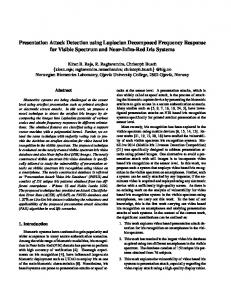
A. Estimator and Controller Mechanization for Altitude Hold To capture the effect of autopilot on tracking the final approach glideslope, we augment an altitude autopilot into the aircraft compensator model. Assuming that there is a spoofing attack during the landing approach, this altitude controller will respond to the spoofing attack by inducing control actions that will be measured by the IMU. To quantify the impact of the aircraft’s autopilot response on RAIM spoofing monitor performance, we utilize a closed loop compensation model including a control feedback obtained from a Kalman filterbased estimator. The block diagram in Fig. 1 illustrates a closed-loop control system with a tightly-coupled INS-GNSS estimator. In this block diagram, true aircraft (A/C) state x is fed to IMU and GNSS sensors which generate measurements for state estimation. Note that the fault f is also added to the system ˆ of the through the GNSS measurements. Using the output x estimator, altitude-hold autopilot produces a control input c (elevator and thrust) resulting in maneuver commands to the aircraft. In this section, we construct a combined estimator-controller mechanization equation. To capture aircraft’s response in this closed loop mechanism, we use an aircraft dynamic model, state-space representation of which is given in Appendix B as x˙ d = F d xd + G

c

(17)

where xd = [ u, w, q, ✓, h]T is aircraft state containing deviation in forward speed u, down speed w, pitch rate q, pitch angle ✓, and altitude h. F d is the plant matrix, G is input coefficient matrix, and c is the control input containing elevator deflection and thrust change, and it is generated based ˆ n as on INS state estimate feedback x c

=

ˆn Kx

(18)

where K is the autopilot gain matrix. On the other hand, the estimator in INS utilizes a kinematic model to predict aircraft motion, which is defined in

Appendix C as

(19)

x˙ n = F n xn + Gu u

where xn = [ r, v, E]T is referred to as the INS state vector including deviations in position vector r, velocity vector v, and attitude vector E of the aircraft. F n is plant matrix of the kinematic model, Gu is input coefficient matrix, and u = [f, !]T is the input provided by IMU measurements including specific force f and angular velocity ! relative to inertial frame. All the states except q in the aircraft state vector xd can be extracted from the INS state vector xn by using proper row eliminations and navigation-to-body frame transformations. Before we define a transformation between them, for analysis purposes, we augment q into xn to account for angular rate information which xd includes but xn does not. The modified 0 INS state xn becomes  0 xn xn = (20) q

variations due to the aircraft controller’s response to spoofing and IMU sensor errors as

where T u extracts specific force and angular velocity terms from aircraft state derivative and converts them to body frame. ⌫ n is a 6 ⇥ 1 vector including accelerometer and gyroscope white noises, which are uncorrelated and zero-mean and b is a 6 ⇥ 1 IMU bias vector that is modeled as a first order Gauss Markov process as b˙ =

where T x extracts aircraft states xd from augmented INS 0 states xn by applying a combination of rotation from navigation to stability frame and row elimination. Pitch rate dynamics is extracted from the aircraft model in (17) as q˙ = T q (F d xd + G c ) (22) where T q extracts the row corresponding to pitch rate q in the aircraft model. To account for the pitch rate dynamics in the INS mechanization, we augment (22) into INS model in (19) as 0



x˙ n q˙

0

=

z

0

Fn }|

Fn 0 TqFdTx

0

0

x G { z }|n { z }|u { xn Gu + u q 0  0 + c TqG | {z } 0 G

(23)

where F n and Gu are the plant and input coefficient matrix of modified INS kinematic model, respectively. Since the aircraft sensors do not provide angular acceleration information ( q), ˙ there is a side process in the INS system that differentiate angular velocity information provided by IMU. This is the reason that we have the second row in (23). Recall that the main aim of introducing an INS kinematic model in (19) and an aircraft dynamic model in (17) is to construct a mechanization equation for the state feedback control system by defining the coupling between these two models. This coupling could be attained through the specific force and angular velocity measurements captured in input vector u in (19). u can be defined as a combination of

1

⌧

(25)

b + ⌘b

where ⌘ b represents the bias driving white noise and ⌧ represents the time constants of biases. Using (17), (18), (21) and (24), the modified INS kinematic model in (23), can be reformulated0 in terms of only the 0 ˆ n , and sensor errors as modified INS state xn , its estimate x 0

0

0

0

x˙ n = F n + Gu T u F d T x xn

0

0

0

ˆn Gu T u G K + G K x 0

0

Now, we can define a direct conversion between xd and xn as 0 xd = T x xn (21)

(24)

u = T u x˙ d + b + ⌫ n

0

+Gu b + Gu ⌫ n

(26)

Augmenting the bias dynamics in (25) with the modified INS model in (26) yields a mechanization equation for actual closed loop control system of the aircraft as 

0

xn b

x #{ z" }|0 #{ Gu xn = 1 b 0 ⌧ " 0 #" 0 #  0 0  Gu T u G K + G K 0 x ˆn Gu 0 ⌫ n + ˆ 0 I ⌘b b 0 0 | {z } | {z } | {z } | {z } w Gw Gc ˆ x (27) z"

F }| F n + Gu T u F d T x 0

0

0

ˆ are the bias augmented INS state and state where x and x estimate vectors, respectively. F , Gc , and Gw are the dynamic, control input coefficient, and noise coefficient matrices of augmented closed loop system, respectively. Discrete form of the closed loop model in (27) is expressed as ˆ k + w wk xk+1 = xk x (28) where is the state transition matrix of the overall closed loop system. and w are discrete forms of Gc and Gw , respectively. For analysis purpose, we assume that INS and control actuation system have the same sampling rates in discretization. So far, we obtained an overall closed loop dynamic model in (28). Fusing this model with the measurement model in Kalman filter will be introduced in the next section. B. Tightly Coupled INS-GNSS Integration To perform a covariance analysis for performance evaluation of the RAIM monitor under GNSS spoofing attacks, GNSS measurement model should be first integrated with the closed loop dynamic model.

Since the main focus of this work is to detect spoofing during landing phase of the flight, we assumed a DD GNSS measurements. The faulted GNSS code and carrier phase measurement equation linearized about a nominal position (Appendix D), can be represented for the k th time epoch as z k = G⇤ r k + DN + ⌫ ⇢

k

+ fk

(29)

where z is the measurement vector containing carrier and code phase measurements after subtracting the nominal, G⇤ is the observation matrix including line-of-sight information from the reference station to the satellites in the navigation frame. r is the variation on the position of the aircraft relative to reference station represented in navigation frame. N and D are the cycle ambiguity state vector and its constant coefficient matrix, respectively and ⌫ ⇢ is the DD carrier and code measurement error vector. f k is the resultant fault vector. By using GNSS-aided INS navigation system, INS error drift is bounded, which allows INS to be used as a consistency check against GNSS spoofing attacks. In tightly coupled mechanism, raw INS and GNSS data are processed in a unified filter [10]. In the tightly coupled integration, coupling between dynamic model and GNSS measurement model can be obtained by first relating the state vector r in GNSS measurement model in (29) to the state vector x used in the closed loop dynamic model in (28) as " # r x= (30) 0 x

spoofer must be f k = f wk

where H and xN are the observation matrix and the state vector of the augmented measurement model, respectively. It should be noted that, although the augmentation of multipath states in (31) is not shown for the sake of simplicity in equations, we take multi path states into account in the implementation, results of which is demonstrated in Section IV. In the existence of the worst-case spoofing attack, measurement z received by the aircraft at time epoch k can be defined as a function of worst-case fault as z k = f wk + ⌫ ⇢

k

(32)

where f w is the worst-case fault vector that the spoofer computes. It should be mentioned that H k xN k term disappears in (32) since the spoofer assumes a nominal flight zero deviation from nominal trajectory xN = 0. k In order for (31) to equal to (32), the relation between resultant fault f k and worst-case fault f wk injected by the

(33)

The difference between the worst-case fault that spoofer assumes, and the resultant fault vector shown in (33) will have an impact on detector, which will be explained in Section III-C in detail. To be consistent with the measurement model in (31), the cycle ambiguity state must also be augmented into the dynamic model in (28) as       ˆk xk+1 0 xk 0 x w = ˆ k + 0 wk N k+1 0 I Nk 0 0 N | {z } | {z } | {z } | {z } | {z } N N N xN ˆN x k w k (34) where N and N are the state transition and state estimate coefficient matrices of the augmented closed loop dynamic system. Superscript N implies cycle ambiguity augmentation. So far, we derived an augmented measurement model in (31) with a closed loop dynamic model in (34) and their short forms can be written as z k = H k xN k + ⌫⇢ xN k+1 =

N

N

xN k

k

(35)

+ fk

ˆN x k +

N w

wk

(36)

A Kalman filter based on equations (35) and (36), has a time update as

0

where x refers to all the states in x except r. Using the relation in (30) and augmenting cycle ambiguity state into x, measurement equation in (29) can be reformulated as 2 3 h i r0k 6 7 z k = G⇤k 0 D 4 xk 5 +⌫ ⇢ k + f k (31) | {z } N Hk | {z } xN k

H k xN k

xN k+1 =

N

|

N

{z ⌥

}

ˆN x k

(37)

N where xN at time epoch k + k+1 is the a priori estimate of x 1. ⌥ is defined for simplicity, which is a function of state transition matrix and the state estimate coefficient matrix of closed loop dynamics. Measurement update at time epoch k + 1 gives the a ˆN posteriori estimate x k+1 as N ˆN x k+1 = xk+1 + Lk+1 z k+1

H k+1 xN k+1

(38)

where Lk+1 is the Kalman gain at time epoch k + 1, and optimally computed as in (10). The only difference between L in (38) and that in (10) is that the one in (38) has extra zero due to the augmentation of the pitch rate state q. However, this does not affect the estimator. Substituting (32) into (38) gives ˆN x k+1 = (I

Lk+1 H k+1 ) xN k+1 + Lk+1 f wk+1 + ⌫ ⇢

k+1

(39) Substituting time update equation (37) into measurement update equation (39) results in ˆN x k+1 = I

ˆN Lk+1 H k+1 ⌥ x k + Lk+1 f wk+1 + ⌫ ⇢

k+1

(40)

False Trajectory

Subtracting (36) from (40) and defining the state estimate ˜N ˆN error x xN k as x k k gives the state estimate error dynamics as ˜N x k+1 =

N

˜N Lk+1 H k+1 ⌥ x k

Lk+1 H k+1 ⌥ xN k

+Lk+1 f wk+1 + ⌫ ⇢

N w

k+1

rf

wk (41)

Dynamic model in (36) can also be written in terms of only ˜ by using the the true state x and the state estimate error x ˆ ˜ relation x = x + x as xN k+1

=

N

⌥ xN k

˜N x k

+

N w

Combining (42) with the estimator error dynamics in (41), we obtain two coupled equation that describe the overall dynamic behavior of the system as " N# " #" N # N xk 1 xk ⌥ = N ˜N x Lk H k ⌥ Lk H k ⌥ x ˜N k k 1 +

"

N w N w

0 Lk

#" wk ⌫⇢

1 k

#

+

Actual Trajectory

! a c

(42)

wk

"

0 Lk

#

f wk (43)

Although state estimate error is not a function of true state in most of the applications [14], it can be seen that there is two-way coupling between the state xN k and its estimate error ˜N x k in (43). The reason is that the resultant fault in the system is a function of actual state as in (33). Using (43), we aim to obtain the time history of the true state xN which represents the deviations from nominal trajectory due to autopilot’s response to the fault in the GNSS measurements. In the closed loop dynamics given in (28), since the current state is a function of previous state estimate which is a random variable, true state will also be a random variable. Let us define NT X k = E{ xN (44) k xk } T ˆ k = E{ x ˜N ˜N P k x k }

Steady-state Response Trajectory

Fig. 2. Impact of the Position Fault and the Consequent Autopilot Response to Spoofing Attack on Aircraft’s Trajectory

deviation is denoted by r. The red trajectory is the steadystate trajectory the aircraft will maneuver and reach to after responding to the spoofed signal. Knowing the nominal path of the aircraft, a smart spoofer may inject the worst-case fault leading to a hazardous situation without being detected by the aircraft monitor [1]. On the other hand, in the existence of autopilot and assuming the spoofer cannot predict the response of the autopilot the resultant fault in the system will be different than the worst-case fault assumed by the spoofer. This increases the detectability of the fault since the actual fault is not the worst case fault anymore, which has a direct impact in the residual. In this work, we assume a worst-case fault f w derived based on a batch estimator, which maximizes integrity risk [1]. In the future work, we will derive worst-case fault based on Kalman filter estimator. Remember that the worst-case fault is computed using nominal trajectory values since it is assumed that the spoofer have knowledge of the nominal trajectory only. Based on (3) and (43), the innovation vector k is k

(45)

ˆ k are true state covariance and state estimate where X k and P error covariance at time epoch k, respectively such that xN k ⇠ ˆ N (ˆ xN k , P k ). C. RAIM Formulation for Fault Detection Performance In this section, we formulate the monitor in terms of the estimator derived for evaluation purpose in the previous section, and derive the integrity risk equations to quantify the monitor performance. Fig. 2 explains the impact of the autopilot response on the aircraft trajectory under spoofing attack. The black dotted line in Fig. 2 is the nominal or planned trajectory. The blue line represents the spoofing trajectory and r f refers to position discrepancy from the nominal due to fault. The black curved trajectory is the actual flight path deviated from the nominal trajectory due to autopilot’s response to spoofing attack. This

Nominal Trajectory

r

= zk

H k xN k

(46)

Substituting (32) into (46) results in k

= f wk + ⌫ ⇢

H k xN k

k

(47)

Using (36) and (37), the innovation vector in (47) can be expressed in terms of true state xk 1 and state estimate error ˜ k 1 as x k

= f wk + ⌫ ⇢

k

H k ( xN k +

N

˜N x k

1

N w wk 1 )

(48)

The new formulation of the innovation vector in (48) captures the autopilot’s response to spoofing attack. Therefore, we can quantify the effect of the controller on the detection capability of RAIM. In order to capture the correlation be˜ k , we augment (48) into (43), which results in tween k and x a complete model containing system dynamics and innovation

as 2

3

y

}|k

z2

xN ⌥ k 6 N7 6 6x 7 6 4 ˜ k 5 = 4 Lk H k ⌥ Hk ⌥ k

N

N

Lk H k ⌥ Hk ⌥

2

N w

6 +6 4

0

3

"

from time epoch 1 to k, the test statistic can be written in terms of 2-norm of 1|k

yk 1 3{ z2 }| 3{ 0 xN k 1 76 N 7 7 6 ˜ k 17 05 4x 5 0 k 1 #

2

0

qk = k

3

7 wk 1 6 7 + 4 L k 5 f wk Lk 7 5 ⌫ ⇢ k I 0 I | {z } | {z } {z } ⌫ yk N w

|

fk

yk

(49)

where y is defined as the state vector of the complete model including true state, state estimate error, and innovation. y , y , and f are the state transition, noise coefficient, and fault input coefficient matrices of the complete system, respectively. Using (49), the mean and covariance of the complete model state y can be propagated as µ yk = Yk =

yk

yk

Yk

µ yk 1

1

+

fk

T yk

+

yk V yk

(50)

f wk T yk

(51)

where µyk and Y k are the mean and covariance of y k , respectively, and V yk is the covariance of ⌫ yk . In Kalman Filter innovation-based RAIM, it was proven that the test statistics obtained from the weighted norm of the innovation using (5) and state estimate error are independent [2]. Therefore, the integrity risk is obtained as a product of the two probabilities as in (14). However, in our case, since the fault is fed into the aircraft by autopilot controller input ˜k through a closed-loop mechanism, the state estimate error x and test statistic qk are no longer independent. Computing the ˜ k and chiintegrity risk with correlated gaussian distribution x square distribution qk is difficult. Therefore, we compute a bound on the integrity risk by first whitening the innovation by its covariance matrix as k

= Sk

1/2

k

(52)

where k is the whitened innovation vector which is a Gaussian and identically distributed in n-space (i.e. E{ k Tk } = I n⇥n ) and S k is the innovation covariance obtained from Y in (51) as Sk = T Y kT T (53) where T and T x˜ extracts the rows of y k corresponding to ˜N k and x k , respectively. Re-expressing the test statistic in (5) in terms of k gives qk =

k X

T n

n

(54)

n=1

[

Defining 1 , 2 , ...,

a cumulative innovation vector = 1|k T ] containing all whitened innovation vectors k

(55)

1|k k2

where 1|k is a Gaussian and identically distributed in n ⇥ k space. n is the number of measurements at each time epoch. Substituting (55) into (6), the detection test can be reexpressed as k 1|k k2 < T 2 (56) The detection test condition in (56) represents a hypersphere which is conservatively over-bounded by a hyperbox as |

1|k |

(57)