arXiv:1409.8526v1 [hep-ph] 30 Sep 2014
GoSam 2.0: a tool for automated one-loop calculations Johann Felix von Soden-Fraunhofen
Max Planck Institute for Physics, Föhringer Ring 6, 80805 Munich, Germany E-mail:
[email protected] Abstract. We present the version 2.0 of the program package GoSam, which is a public program package to compute one-loop QCD and/or electroweak corrections to multi-particle processes within and beyond the Standard Model. The extended version of the Binoth-LesHouches-Accord interface to Monte Carlo programs is also implemented. This allows a large flexibility regarding the combination of the code with various Monte Carlo programs to produce fully differential NLO results, including the possibility of parton showering and hadronisation. We illustrate the wide range of applicability of the code by showing phenomenological results for multi-particle processes at NLO, both within and beyond the Standard Model.
1. Introduction In the last years, there has been a remarkable progress in the development of automated NLO tools for multi-particle processes. This leads to the possibility of having NLO corrections matched to parton-showers as the new standard at the LHC. Here we want to summarize the new features of the GoSam 2.0 release [1], which is able to automatically compute one-loop QCD and/or electroweak corrections to user-defined processes, and show the results of two applications. The developments since the former release of GoSam described in [2, 3] has allowed various phenomenological studies within and beyond the Standard model [4–15]. The new features are now publicly available in the GoSam 2.0 release. 2. GoSam 2.0 workflow GoSam can be used standalone to generate code for one-loop amplitudes1 or in combination with recent Monte Carlo programs via the Binoth-Les-Houches-Accord (BLHA) described in Sec. 3.1. In the standalone mode, which is shown schematically in Fig. 1, the user provides the needed information to GoSam via an input card. GoSam calls QGraf [16] to generate all Feynman diagrams and the related algebraic expressions. These are further processed by FORM [17, 18]. The spinor algebra is handled by the Spinney library [19]. The code is then transformed to compilable expressions using the new FORM 4 features [18] (see Sec. 3). At runtime, the generated code can choose between different integrand-level reduction methods [20, 21], implemented in Ninja [22–24] and Samurai [25, 26], and improved tensor reduction methods implemented in Golem95 [27–30]. 1
The generation of colour/spin correlated tree level amplitudes is also possible.
Input file process.in
GoSam
GoSam gosam.py process.in Diagrams drawing and code generation QGraf, FORM, Spinney
Reduction: Ninja | Golem95C | Samurai | . . . Integral library: OneLOop | Golem95C | QCDLoop | . . . Virtual one-loop amplitude BLHA1/BLHA2 interface
direct linking
Monte Carlo event generator Madgraph/Maddipole, Sherpa, PowhegBox, Herwig++, . . .
Figure 1. Basic workflow of GoSam 3. New features of GoSam 2.0 In this section we present some highlights of the version 2.0 of GoSam. Higher rank integrals While in calculations in Feynman gauge within in the Standard Model, the tensor rank is always smaller or equal to the number of propagators in a loop integral, this is not necessarily the case in other gauges, effective theories or theories with spin-2 particles. For the GoSam 2.0 release, all of the supported reduction libraries (Ninja, Samurai, Golem95) have been extended to the case where the rank of the tensor integrals exceeds the number of the propagators [22, 26, 30]. New reduction method In GoSam 2.0, the new default reduction library is Ninja [22–24]. Ninja is a new developed integrand-reduction method and exploits the fact that the integrands are provided by GoSam in analytic expressions. It uses the Laurent expansion of the integrands performed by semi-numerical polynomial divisions. Improved code generation The generation of optimized code is now mainly handled by the new FORM 4.0 optimization features [18, 31], which enables faster and more compact code. Grouping and summing of diagrams with common substructure GoSam 2.0 has a new option diagsum which automatically groups or combines diagrams which share a common loop-structure and/or which can be distinguished only by external tree parts. This reduces not only the code generation time, but also the number of calls to the reduction method and, therefore, increases the overall performance. This extends the option of grouping diagrams already present in GoSam 1.0. Numerical polarisation vectors By default, GoSam 2.0 creates code with generic polarisation vectors for massless gauge bosons and evaluates it for the various helicity configurations numerically. This saves the generation of separate code for each helicity configuration and therefore reduces the code generation time and the disk and memory footprint. Improved tensorial reconstruction The new GoSam release enables by default the derive extension, which allows to isolate the tensor coefficients entering tensorial reconstruction [32] in
a more efficient way. It is based on the fact that the numerator can be written as a (tensorial) Taylor series in the loop momenta q µ around q = 0. Electroweak scheme choices GoSam 2.0 supports various schemes defining which of the electroweak parameters are input parameters and which ones are derived parameters. From a certain set of input parameters defining an electroweak scheme, GoSam will automatically determine the derived parameters. If not otherwise specified, GoSam uses the set (MW , MZ , α) by default. The settings can be provided to GoSam using the model.options keyword, which also needs to contain ewchoice if the choice should be changeable at runtime. If GoSam is accessed via the Binoth Les Houches interface (cf. Sec. 3.1), the electroweak scheme is determined automatically according to the OLP_SetParameter calls. 3.1. BLHA2 Interface GoSam 2.0 supports the Binoth Les Houches Accord 2 (BLHA2), an updated standard interface between Monte Carlo event generators and one-loop programs [33]. The first version of the BLHA standard [34] is still supported. 1. Order file ? 2. Contract file X
Code generation Building
Monte Carlo event generator Sherpa, PowhegBox, Herwig++, aMC@NLO, . . .
gosam.py –olp OrderFile.lh
phase space point, scale, . . . result, accuracy
generated GoSam code
dynamical linking Reduction libraries: Ninja, Samurai, Golem95
NLO result
Figure 2. Workflow of the BLHA2 interface with GoSam The workflow of this interface is described in Fig. 2. It can be split into two phases. The first phase is the “order/contract phase”, where the Monte Carlo programs “asks” the one-loopprovider (e.g. GoSam) for the needed processes in an order file. It can then “reply” with an contract file and generate the code. As soon as the contract is “signed”, i. e. all the items placed in the order file can be provided, the second phase can start. The Monte Carlo program is able to dynamically link the generated code for the virtual amplitude and can evaluate the amplitude at phase space points, thus performing the integration and event generation steps. The updated interface allows to specify processes with different multiplicities and settings in one order file. GoSam can also provide colour- and spin-correlated LO matrix elements. Both features allows the Monte Carlo program to built subtraction terms of NLO real radiation in addition to the virtual part. The accuracy can be assessed by various tests: The first test compares the infrared pole coefficients to those obtained from the general structure of infrared singularities. The second, more time-consuming test is a rotation test, where the scattering amplitude is re-evaluated after an azimuthal rotation around the beam axis, which should keep the amplitude invariant. The thresholds triggering the various tests can be adjusted by the user via the input card.
These tests are also used to trigger the rescue system (switching to Golem95 as reduction library) in the case of unstable results and are, if necessary, repeated to obtain the estimated accuracy of the final (rescued) result. This procedure has been shown to be a good compromise between speed and quality of the assessed accuracy. 4. Installation GoSam 2.0 is distributed with a new install script, which installs the code automatically. It also helps to update GoSam and its components. The install script can be downloaded by calling wget http://gosam.hepforge.org/gosam-installer/gosam_installer.py The next step is to run the installer with the following commands chmod +x gosam_installer.py ./gosam_installer.py --prefix=path/to/install or alternatively: python gosam_installer.py --prefix=path/to/install If the --prefix option is left out, the script installs GoSam into a subdirectory ./local of the current working directory. Upon installation, the installer asks the user if it should use existing programs on the system (FORM 4, QGraf, reduction libraries) or should install new versions of them which are tested with GoSam. For a default installation, the questions can be safely answered by pressing the ENTER key. After this, the installer downloads, builds and installs all components. Finally, a script [prefix]/bin/gosam_setup_env.sh is created which sets up (temporarily) all environment variables if sourced in a shell. It is suggested to keep the installer-log.in, which may be needed to update or uninstall GoSam later. The update process can be initiated by calling the install script again without any arguments in the same folder where this file is located. 5. Using GoSam By calling gosam.py --template process.in, the user is able to generate an input file where all possible settings are explained and default settings are shown. After filling all settings, gosam.py process.in generates a subdirectory specified by the process_path setting in the input card. The remaining steps for code generation and building can be performed by calling make source and make compile in this process directory. In the doc/ subfolder, make doc generates documentation containing process specific informations as well as Feynman diagrams. The matrix/ subdirectory contains a file test.f90 which contains an example how to interface the compiled code. It can be built by calling make test.exe and outputs the NLO result for one random phase space point by default. An example input-file for QCD corrections to e+ e− → tt¯ is shown in Fig. 3. process_name=eett process_path=eett_code in=e+,eout=t,t order=QCD,0,2 one=gs,e zero=me,mU,mD,mS,mC,mB
Figure 3. Example of an input card for QCD corrections to e+ e− → tt¯
6. Applications 6.1. First example of GoSam plus Herwig++/Matchbox As a first example demonstrating the features of the BLHA2 interface implemented in GoSam 2.0 and an upcoming version of Herwig++/Matchbox [35–37], the NLO QCD corrections to the process pp → Z/γ ∗ + jet → e+ e− + jet were calculated. dσ/d∆R(Z,j1 ) [pb]
Separation between Z boson and leading jet b b
10 2
b b
b
b b
b
10 1
10−1
b
b
1
2
b b
b b
b
1
b
b b
3
b
Herwig++/Matchbox GoSam GoSam + PS Herwig++/Matchbox + PS 4
5
6
b
b b
7 ∆R(Z,j1 )
Figure 4. Z+jet production: R separation between the Z-boson and the leading jet. The blue dots and the green line show the result of Herwig++/Matchbox using matrix elements generated by GoSam without and with parton shower; the red and pink lines show the corresponding results with built-in Herwig/Matchbox matrix elements. Besides the virtual matrix elements, GoSam provides various tree-level matrix elements (normal Born matrix elements and spin- and colour-correlated Born matrix elements) via the BLHA2 interface, which supports now order files with subprocesses of different amplitude types and multiplicities. This allows Herwig++ to calculate the full NLO real radiation part. As this specific process is also directly built-in in Herwig++/Matchbox, it was easily possible to validate the results. Fig. 4 shows the matching results. Both ways are largely automated, i.e. only small changes in the Herwig++ input card (and optionally in an additional GoSam setting card) are needed. Furthermore, Herwig++ can match a parton shower to the fixed-order calculation, which gives access to new kinematical regions. The result is also plotted in Fig. 4. Full details of this calculation and information about the implementations can be found in [38]. 6.2. Diphoton plus jet production through graviton exchange The NLO QCD corrections to the production of a photon pair through graviton exchange in association with a jet has been calculated with GoSam within the ADD model [39, 40], which assumes flat, large extra dimensions. The model file was generated by FeynRules [41] and imported into GoSam using the UFO file format [42]. Four to six extra dimensions were assumed and an ADD scale MS = 4 TeV was chosen. According to this scale, the invariant mass of the photon pair was restricted to 140 GeV ≤ mγγ ≤ 3.99 TeV. A variation of this upper cut-off showed that the results are not considerably affected by the unknown UV completion of the ADD model. Since rank-5 boxes and rank-4 triangles appear, the higher rank extensions of GoSam and Golem95C (cf. Sec. 3) were used. Additionally, the sum over all discrete Kaluza-Klein mode propagators was approximated by a density function, which required a new custompropagator extension in GoSam, and a Lorentz structure where on-shell conditions were assumed. All of the needed features are available in the Golem95 1.3 and GoSam 2.0 release. For this process, large enhancements are expected in the tail of the diphoton mass spectrum which is shown in Fig. 5. In particular, we observe a non-constant K-factor for this observable, which existing experimental searches have not considered. More details and results can be found in [15], including the case of five and six extra dimensions.
dσ/dm(γ1 , γ2 ) [pb/GeV]
10−6
10−7
10−8
10−9 LO NLO
K-factor
10−10 1.4 1.2 1 0.8 0.6 0
500
1000
1500
2000
2500
3000
3500
4000
m(γ1 , γ2) [GeV]
Figure 5. NLO corrections to the invariant di-photon mass distribution stemming from the graviton decay √ including a scale variation by a factor two around the central scale in proton-proton collisions at s = 8 TeV 7. Conclusion GoSam 2.0 provides many new features, leading to faster and more compact code, increased usability and a broader range of possible applications. In particular, GoSam supports now higher-rank integrals, where the tensor rank exceeds the number of propagators. This is needed in effective field theories and in calculations with spin-2 particles. Furthermore, complex masses and couplings, and various electroweak schemes are supported. A new installation script simplifies the installation of GoSam and related libraries and tools. The overall performance was greatly increased by introducing a new integrand-level reduction method, implemented in the Ninja library, by advanced techniques of combining and grouping Feynman diagrams and by using the new FORM 4 features for code optimization. Many of the new features were already successfully used and tested in various phenomenological studies [4–15]. The implementation of the new standardized interface to Monte Carlo programs (BLHA2) allows to use parton showered events at NLO level and to use different Monte Carlo generators for comparisons. Acknowledgements The author thanks all the current and former members of the GoSam collaboration for the joint effort in developing GoSam 2.0. Furthermore, he is grateful to the members of the Herwig++ collaboration for the common work on combining both programs via the BLHA2 interface, and Joscha Reichel for his contribution to the diphoton plus jet through graviton exchange calculation. References
[1] Cullen G, van Deurzen H, Greiner N, Heinrich G, Luisoni G, Mastrolia P, Mirabella E, Ossola G, Peraro T, Schlenk J, von Soden-Fraunhofen J F and Tramontano F 2014 Eur.Phys.J. C74 3001 (Preprint 1404.7096) [2] Reiter T 2009 Automated Evaluation of One-Loop Six-Point Processes for the LHC Ph.D. thesis (Preprint 0903.0947) [3] Cullen G, Greiner N, Heinrich G, Luisoni G, Mastrolia P et al. 2012 Eur.Phys.J. C72 1889 (Preprint 1111.2034)
[4] Greiner N, Heinrich G, Mastrolia P, Ossola G, Reiter T et al. 2012 Phys.Lett. B713 277–283 (Preprint 1202.6004) [5] van Deurzen H, Greiner N, Luisoni G, Mastrolia P, Mirabella E et al. 2013 Phys.Lett. B721 74–81 (Preprint 1301.0493) [6] Gehrmann T, Greiner N and Heinrich G 2013 JHEP 1306 058 (Preprint 1303.0824) [7] Luisoni G, Nason P, Oleari C and Tramontano F 2013 JHEP 1310 083 (Preprint 1306.2542) [8] Hoeche S, Huang J, Luisoni G, Schoenherr M and Winter J 2013 Phys.Rev. D88 014040 (Preprint 1306.2703) [9] Cullen G, van Deurzen H, Greiner N, Luisoni G, Mastrolia P et al. 2013 Phys.Rev.Lett. 111 131801 (Preprint 1307.4737) [10] van Deurzen H, Luisoni G, Mastrolia P, Mirabella E, Ossola G et al. 2013 Phys.Rev.Lett. 111 171801 (Preprint 1307.8437) [11] Gehrmann T, Greiner N and Heinrich G 2013 Phys.Rev.Lett. 111 222002 (Preprint 1308.3660) [12] Dolan M J, Englert C, Greiner N and Spannowsky M 2014 Phys.Rev.Lett. 112 101802 (Preprint 1310.1084) [13] Heinrich G, Maier A, Nisius R, Schlenk J and Winter J 2014 JHEP 1406 158 (Preprint 1312.6659) [14] Cullen G, Greiner N and Heinrich G 2013 Eur.Phys.J. C73 2388 (Preprint 1212.5154) [15] Greiner N, Heinrich G, Reichel J and von Soden-Fraunhofen J F 2013 JHEP 1311 028 (Preprint 1308.2194) [16] Nogueira P 1993 J.Comput.Phys. 105 279–289 [17] Vermaseren J 2000 (Preprint math-ph/0010025) [18] Kuipers J, Ueda T, Vermaseren J and Vollinga J 2013 Comput.Phys.Commun. 184 1453–1467 (Preprint 1203.6543) [19] Cullen G, Koch-Janusz M and Reiter T 2011 Comput.Phys.Commun. 182 2368–2387 (Preprint 1008.0803) [20] Ossola G, Papadopoulos C G and Pittau R 2007 Nucl.Phys. B763 147–169 (Preprint hep-ph/0609007) [21] Giele W T, Kunszt Z and Melnikov K 2008 JHEP 0804 049 (Preprint 0801.2237) [22] Mastrolia P, Mirabella E and Peraro T 2012 JHEP 1206 095 (Preprint 1203.0291) [23] van Deurzen H, Luisoni G, Mastrolia P, Mirabella E, Ossola G et al. 2014 JHEP 1403 115 (Preprint 1312.6678) [24] Peraro T 2014 Comput.Phys.Commun. 185 2771–2797 (Preprint 1403.1229) [25] Mastrolia P, Ossola G, Reiter T and Tramontano F 2010 JHEP 1008 080 (Preprint 1006.0710) [26] van Deurzen H 2013 Acta Phys.Polon. B44 2223–2230 [27] Binoth T, Guillet J P, Heinrich G, Pilon E and Schubert C 2005 JHEP 0510 015 (Preprint hep-ph/0504267) [28] Binoth T, Guillet J P, Heinrich G, Pilon E and Reiter T 2009 Comput.Phys.Commun. 180 2317–2330 (Preprint 0810.0992) [29] Cullen G, Guillet J P, Heinrich G, Kleinschmidt T, Pilon E et al. 2011 Comput.Phys.Commun. 182 2276–2284 (Preprint 1101.5595) [30] Guillet J P, Heinrich G and von Soden-Fraunhofen J 2014 Comput.Phys.Commun. 185 1828–1834 (Preprint 1312.3887) [31] Kuipers J, Ueda T and Vermaseren J 2013 (Preprint 1310.7007) [32] Heinrich G, Ossola G, Reiter T and Tramontano F 2010 JHEP 1010 105 (Preprint 1008.2441) [33] Alioli S, Badger S, Bellm J, Biedermann B, Boudjema F et al. 2014 Comput.Phys.Commun. 185 560–571 (Preprint 1308.3462) [34] Binoth T, Boudjema F, Dissertori G, Lazopoulos A, Denner A et al. 2010 Comput.Phys.Commun. 181 1612–1622 (Preprint 1001.1307) [35] Bellm J, Gieseke S, Grellscheid D, Papaefstathiou A, Plätzer S et al. 2013 (Preprint 1310.6877) [36] Plätzer S and Gieseke S 2012 Eur.Phys.J. C72 2187 (Preprint 1109.6256) [37] Bahr M, Gieseke S, Gigg M, Grellscheid D, Hamilton K et al. 2008 Eur.Phys.J. C58 639–707 (Preprint 0803.0883) [38] Bellm J, Gieseke S, Greiner N, Heinrich G, Plätzer S, Reuschle C and von Soden-Fraunhofen J 2014 Gosam plus herwig++/matchbox Les Houches 2013: Physics at TeV Colliders: Standard Model Working Group Report (Preprint 1405.1067) [39] Arkani-Hamed N, Dimopoulos S and Dvali G 1998 Phys.Lett. B429 263–272 (Preprint hep-ph/9803315) [40] Antoniadis I, Arkani-Hamed N, Dimopoulos S and Dvali G 1998 Phys.Lett. B436 257–263 (Preprint hepph/9804398) [41] Christensen N D and Duhr C 2009 Comput.Phys.Commun. 180 1614–1641 (Preprint 0806.4194) [42] Degrande C, Duhr C, Fuks B, Grellscheid D, Mattelaer O et al. 2012 Comput.Phys.Commun. 183 1201–1214 (Preprint 1108.2040)