Gossip protocols for large-scale distributed systems - SBRC'2010

Gossip protocols for large-scale distributed systems Alberto Montresor

© Alberto Montresor

1

University of Trento


2


3

Gossip definition ✦

✦

In a recent workshop on the future of gossip ✦

many attempts to formally define gossip

✦

we failed! ✦

either too broad

✦

or too strict

Gossip best described with a prototypical gossip scheme ✦

“I cannot define gossip, but I can recognize it when I see it”


4

A generic gossip protocol - executed by process p

Init: initialize my local state Active thread

do once every δ time units q = getPeer(state) sp = prepareMsg(state, q) send (REQ, sp, p) to q

Passive thread

do forever receive (t, sq, q) from * if ( t = REQ ) then sp = prepareMsg(state, q) send (REP, sp, p) to q state = update(state, sq)

A "cycle" of length δ


5

Epidemic cycle ✦

During a cycle of length δ, every node has the possibility of contacting one random node


6

A generic gossip protocol ✦

Generic scheme is... too generic!

✦

Gossip “rules of thumb” ✦

peer selection must be random, or at least guarantee enough peer diversity

✦

only local information is available at all nodes

✦

communication is round-based (periodic)

✦

transmission and processing capacity per round is limited

✦

all nodes run the same protocol


7

A bit of history ✦

1987 ✦

✦

'90s ✦

✦

Gossip applied to solve communication problems

'00s ✦

✦

Demers et al. introduced the first gossip protocol, for information dissemination

Gossip revival: beyond dissemination

2006 ✦

First workshop on the future of gossip, Leiden (NL)


8

What is going on? ✦

In the last decade, we have seen dramatic changes in the distributed system area

✦

Shift in the scale of distributed systems

✦

✦

larger

✦

geographically more dispersed

Traditional failure model do not hold any more ✦

“let p1 ... pn be a set of processes...”

✦

f < 3n+1, f r.value.time then

Rumor

r.value ← p.value ✦

Pull if p.value.time < r.value.time then

Rumor

p.value ← r.value ✦

Push-pull if p.value.time > r.value.time then

Push

Rumor

r.value ← p.value else p.value ← r.value


Pull Rumor

24

Anti-entropy


25

Anti-entropy


25

Anty-entropy: Convergence


26

Anty-entropy: Convergence ✦

To analyze convergence, we must consider what happens when only a few nodes remain susceptible ✦

Let p(i) be the probability of a node being (remaining) susceptible after the i-th anti-entropy cycle. ✦


Pull:

26




✦


Pull: ✦ p(i+1) = p(i)2 Push:

26




✦

✦

✦

Pull: ✦ p(i+1) = p(i)2 Push: ✦ p(i+1) = p(i)(1 - 1/n)n(1-p(i)) For small p(i), p(i+1) ~ p(i)/e Push-pull: ✦ both mechanisms are used, convergence is even more rapid

All converge to 0, but pull is more rapid than push, so in practice pull (or push-pull) is used


26

Push vs pull


27

Anti-entropy: Comments ✦

Benefits: ✦

✦

✦

For a push implementation, the expected time to infect everyone is log2(n) + ln(n)

Drawbacks: ✦

✦

✦

Simple epidemics eventually “infect” all the population

Propagates updates much slower than best effort Requires examining contents of database even when most data agrees, so it cannot practically be used too often

Normally used as support for best effort, i.e. left running in the background


28

Anti-entropy: Optimizations ✦

To avoid expensive databases checks: ✦

Maintain checksum, compare databases if checksums unequal

✦

Maintain recent update lists for time T, exchange lists first

✦

✦

Maintain inverted index of database by timestamp; exchange information in reverse timestamp order, incrementally re-compute checksums

Note: ✦

✦

These optimizations apply to the update problem for large DB We will see how the same principle (anti-entropy) may be used for several other kind of applications


29

Rumor mongering - complex epidemics ✦

Susceptive-infective-removed (SIR) ✦

Nodes initially susceptive

✦

When a node receives a new update it becomes a “hot rumor” and the node infective

✦

✦

✦

A node that has a rumor periodically chooses randomly another node to spread the rumor Eventually, a node will “lose interest” in spreading the rumor and becomes removed ✦

Spread too many times

✦

Everybody knows it

Optimizations ✦

A sender can hold (and transmit) a list of infective updates rather than just one.


30

Rumor mongering


31

Rumor mongering


31

Rumor mongering


31

Rumor mongering


31

Rumor mongering: loss of interest ✦

✦

Counter vs. coin (random) ✦

Coin (random): lose interest with probability 1/k

✦

Counter: lose interest after k contacts

Feedback vs blind ✦

Feedback: lose interest only if the recipient knows the rumor.

✦

Blind: lose interest regardless of the recipient.


32

Rumor mongering ✦

How fast does the system converge to a state where all nodes are not infective? (inactive state) ✦

✦

Eventually, everybody will lose interest

Once in this state, what is the fraction of nodes that know the rumor? ✦

The rumor may stop before reaching all nodes


33

Rumor mongering: analysis ✦

Analysis from “real” epidemics theory

✦

Feedback, coin ✦

Let s, i and r denote the fraction of susceptible, infective, and removed nodes respectively. Then: s+i+r =1 ds/dt = −si

di/dt = +si − (1/k)(1 − s)i

✦

Solving the equations: s = e−(k+1)(1−s)

✦

Thus, increasing k we can make sure that most nodes get the rumor, exponentially better


34

Quality measures ✦

✦

✦

Residue: ✦

The nodes that remain susceptible when the epidemic ends: value of s when i = 0

✦

Residue must be as small as possible

Traffic: ✦

The average number of database updates sent between nodes

✦

m = total update traffic / # of nodes

Delay - We can define two delays: ✦

tavg : average time it takes for the introduction of an update to reach a node.

✦

tlast : time it takes for the last node to get the update.


35

Simulation results Using feedback and counter Counter k

Residue s

Traffic m

1

0.176

2

Convergence tavg

tlast

1.74

11.0

16.8

0.037

3.30

12.1

16.9

3

0.011

4.53

12.5

17.4

4

0.0036

5.64

12.7

17.5

5

0.0012

6.68

12.8

17.7

Using blind and random


Counter k

Residue s

Traffic m

1

0.960

2

Convergence tavg

tlast

0.04

19

38

0.205

1.59

17

33

3

0.060

2.82

15

32

4

0.021

3.91

14.1

32

5

0.008

4.95

13.8

32

36

Push and pull ✦

Push (what we have assumed so far) ✦

✦

✦

If database becomes quiescent, this scheme stops trying to introduce updates. If there are many independent updates, more likely to introduce unnecessary messages.

Pull ✦

✦

If many independent updates, pull is more likely to find a source with a non-empty rumor list But if database quiescent, it spends time doing unnecessary update requests.


37

Push and pull ✦

Empirically, in the database system of the authors (frequent updates) ✦

✦

Pull has a better residue/traffic relationship than push

Performance of pull epidemic on 1000 nodes using feedback & counters


Counter k

Residue s

Traffic m

1 2 3

0.031 0.00058 0.000004

2.70 4.49 6.09

Convergence tavg 9.97 10.07 10.08

tlast 17.63 15.39 14.00

38

Mixing with anti-entropy ✦

Rumor mongering ✦

✦

✦

spreads updates fast with low traffic however, there is still a nonzero probability of nodes remaining susceptible after the epidemic

Anti-entropy ✦

✦

can be run (infrequently) in the background to ensure all nodes eventually get the update with probability 1. Since a single rumor that is already known by most nodes dies out quickly


39

Deletion and death certificates ✦

Deletion ✦

✦

✦

We cannot delete an entry just by removing it from a node - the absence of the entry is not propagated. If the entry has been updated recently, there may still be an update traversing the network!

Death certificate ✦

Solution: replace the deleted item with a death certificate (DC) that has a timestamp and spreads like an ordinary update


40

Deletion and death certificates ✦

Problem: ✦

✦

✦

we must, at some point, delete DCs or they may consume significant space

Strategy 1: ✦

retain each DC until all nodes have received it

✦

requires a protocol to determine which nodes have it and to handle node failures

Strategy 2: ✦

✦

hold DCs for some time (e.g. 30 days) and discard them pragmatic approach, still have the “resurrection” problem; increasing the time requires more space


41

Spatial Distribution ✦

In the previous exposition ✦

✦

The network has been considered uniform (i.e. all nodes equally reachable)

In reality ✦

✦

✦

More expensive to send updates to distant nodes Especially if a critical link needs to be traversed Traffic can clog these links


42

Peer sampling ✦

Bibliography ✦

✦

✦

✦

S. Voulgaris, D. Gavidia, and M. Van Steen. Cyclon: Inexpensive membership management for unstructured p2p overlays. Journal of Network and Systems Management, 13(2):197–217, 2005 M. Jelasity and M. van Steen. Large-scale newscast computing on the Internet. Technical Report IR-503 (October), Vrije Universiteit Amsterdam, Department of Computer Science, Amsterdam, The Netherlands. M. Jelasity, S. Voulgaris, R. Guerraoui, A.-M. Kermarrec, and M. van Steen. Gossipbased peer sampling. ACM Transactions on Computer Systems, 25(3):8, August 2007 G. P. Jesi, A. Montresor, and M. van Steen. Secure peer sampling. Computer Networks, 2010. To appear.


43

Peer sampling ✦

✦

✦

The first problem to be solved: ✦

Where getPeer() get nodes from?

✦

We assumed complete knwoledge of the distributed system

But complete knowledge is costly ✦

System is dynamic

✦

Network can be extremely large

Solution: peer sampling ✦

Provides random samples from the participant set

✦

Keeps the participants together in a connected network


44

Can you spot the difference? ✦

Traditional gossip ✦

✦

Each node has full view of the network Each node periodically “gossips” with a random node, out of the whole set


✦

Peer sampling ✦

✦

Nodes have a partial view of the network (a set of “neighbors”) Each node periodically “gossips” with a random node, out of its partial view

45

Overlay ✦

✦

An overlay network is a logical network overimposed on a physical network ✦

Nodes

✦

Logical links between nodes

Examples ✦

Structured overlay network ✦

✦

DHTs, trees

Unstructured overlay network ✦

Gnutella

✦

Bittorrent

✦

etc.


System model ✦

✦

A dynamic collection of distributed nodes that want to participate in a common epidemic protocol ✦

Node may join / leave

✦

Node may crash at any time

Churn

Communication: ✦

To communicate with node q, node p must know its address

✦

Messages can be lost – high levels of message omissions can be tolerated


Our Overlays ✦

State of each node: ✦

✦

✦

✦

✦

The address needed to communicate with p

Vie

A

A, 7

(c = view size)

Descriptors of node p contains ✦

B

A partial view containing c descriptors

C

C, 9 E, 10 E

D

F

Additional information that may be needed by different implementations of the peer sampling service Additional information that may be needed by upper layers


48



do once every δ time units q = getPeer(state) sp = prepareMsg(state, q) send (REQ, sp) to q

Passive thread

do forever receive (t, sq ) from * if ( t = REQ ) then sp = prepareMsg(state, q) send (REP, sp) to q state = update(state, sq)



49

A generic algorithm ✦

getPeer() ✦

✦

✦

select one of the neighbor contained in the view

prepareMsg(view, q) ✦

returns a subset of the descriptors contained in the local view

✦

may add other descriptors (e.g. its own)

update(view, msgq) ✦

returns a subset of the descriptors contained in the union of the local view and the received view


50

Newscast ✦

Descriptor: address + timestamp

✦

getPeer() ✦

✦


✦

select one node at random

returns the entire view + a local descriptor with a fresh timestamp


returns the C freshest identifiers (w.r.t. timestamp) from the union of local view and message


51

Newscast


Newscast

ID & Time Address stamp

9 12 16



7 10 14

Newscast



9 12 16

7 10 14

1. Pick random peer from my view © Alberto Montresor

Newscast



9 12 16

7 10 14

1. Pick random peer from my view © Alberto Montresor

Newscast



9 12 16

7 10 14

1. Pick random peer from my view 2. Send each other view + own fresh link © Alberto Montresor

Newscast



9 12 16

7 10 14 9 12 16 20 1. Pick random peer from my view 2. Send each other view + own fresh link


Newscast



9 12 16

7 10 14

7 10 14

9 12 16

20

20 1. Pick random peer from my view 2. Send each other view + own fresh link


Newscast


9 12 16


7 10 14

7 10 14

9 12 16

20

20


1. Pick random peer from my view 2. Send each other view + own fresh link 3. Keep c freshest links (remove own info, duplicates)

Newscast


9 12 16


7 10 14

7 10 14

9 12 16

20

20


1. Pick random peer from my view 2. Send each other view + own fresh link 3. Keep c freshest links (remove own info, duplicates)

Newscast


14 16 20



14 16 20

1. Pick random peer from my view 2. Send each other view + own fresh link 3. Keep c freshest link (remove own info, duplicates)

Newscast ✦

Experiments ✦

100,000 nodes

✦

C = 20 neighbors per node


55

Evaluation framework ✦

Average path length ✦

✦

The average of shortest path lengths over all pairs of nodes in the graph

In epidemic dissemination protocols ✦

A measure of the time needed to diffuse information from a node to another


56

Evaluation framework ✦

Clustering coefficient ✦

✦

✦

✦

✦

The clustering coefficient of a node p is defined as the # of edges between the neighbors of p divided by the # of all possible edges between those neighbors Intuitively, indicates the extent to which the neighbors of p know each other. The clustering cofficient of the graph is the average of the clustering coefficients of all nodes Examples ✦

for a complete graph it is 1

✦

for a tree it is 0

In epidemic dissemination protocols ✦

High clustering coefficient means several redundant messages are sent when an epidemic protocol is used


57


Indication of the time and cost to flood the network


58


High clustering is bad for: ✦

Flooding: It results in many redundant messages

✦

Self-healing: Strongly connected cluster → weakly connected to the rest of the network

- High clustering - Low diameter © Alberto Montresor

}

Newscast forms a SMALL WORLD 59

In-Degree Distribution ✦

Affects: ✦

✦

✦

Robustness (shows weakly connected nodes) Load balancing The way epidemics spread


Robustness

Sustains up to 68% node failures Random sustains up to 80%


Self-healing behaviour


Cyclon ✦

Descriptor: address + timestamp

✦

getPeer()

✦

✦

select the oldest descriptor in the view

✦

remove it from the view


In active thread: ✦

✦

In passive thread: ✦

✦

returns a subset of t-1 random nodes, plus a fresh local identifier returns a subset of t random nodes


discard entries in msgq: p, nodes already know

✦

add msgq , removing entries sent to q


Cyclon


9 12 4



7 10 14

Cyclon



9 12 4

7 10 14

1. Pick oldest peer from my view © Alberto Montresor

Cyclon



9 12 4

7 10 14

1. Pick oldest peer from my view © Alberto Montresor

Cyclon



9 12 4

7 10 14

1. Pick oldest peer from my view 2. Exchange some neighbors (the pointers) © Alberto Montresor

Cyclon



9

7 10 14 12

4


Cyclon



9

7 10 14 12 4


Cyclon



9

7 10 14 12 20


Cyclon



9 7

10 14 12 20


Cyclon



9 7 10

14 12 20


Cyclon Guaranteed connectivity ID & Time Address stamp


9 7 10

14 12 20


Obvious advantages of Cyclon ✦

Connectivity is guaranteed

✦

Uses less bandwidth ✦

Only small part of the view is sent


65


Indication of the time and cost to flood the network


66




✦



67




✦


- Low clustering - Low diameter


}

Cyclon approx. a RANDOM GRAPH

68

In-Degree Distribution ✦

Affects: ✦

✦

✦

Robustness (shows weakly connected nodes) Load balancing The way epidemics spread


Robustness

Sustains up to 80% node failures





Killed 50,000 nodes at cycle 19


Non-symmetric overlays ✦

Non-uniform period → Non symmetric topologies ✦

A node’s in-degree is proportional to its gossiping frequency

✦

Can be used to create topologies with “super-nodes”


73

Secure peer sampling ✦

This approach is vulnerable to certain kinds of malicious attacks

✦

Hub attack ✦

✦

✦

✦

✦

Hub attack involves some set of colluding nodes always gossiping their own ID’s only This causes a rapid spread of only those nodes to all nodes - we say their views become “polluted” At this point all non-malicious nodes are cut-off from each other The malicious nodes may then leave the network leaving it totally disconnected with no way to recover Hence the hub attack hijacks the speed of the Gossip approach to defeat the network


74

Secure peer sampling


Peer sampling - solution ✦

Algorithm ✦

Maintain multiple independent views in each node

✦

During a gossip exchange measure similarity of exchanged views

✦

With probability equal to proportion of identical nodes in two views reject the gossip and blacklist the node

✦

Otherwise, whitelist the node and accept the exchange

✦

Apply an aging policy to to both white and black lists

✦

When supplying a random peer to API select the current “best” view


76

Secure peer sampling




1000 nodes



20 malicious nodes

How to compose peer sampling

Information dissemination

Aggregation prepareMsg() update()

prepareMsg() update()

getPeer()

getPeer()

Peer sampling

Peer sampling

getPeer()



getPeer()


78

Aggregation ✦

Bibliography ✦

✦

Márk Jelasity, Alberto Montresor, and Ozalp Babaoglu. Gossip-based aggregation in large dynamic networks. ACM Trans. Comput. Syst., 23(1):219-252, August 2005.

Additional bibliography ✦

Alberto Montresor, Márk Jelasity, and Ozalp Babaoglu. Decentralized ranking in large-scale overlay networks. In Proc. of the 1st IEEE Selfman SASO Workshop, pages 208-213, Isola di San Servolo, Venice, Italy, November 2008.


79

Aggregation ✦

Definition ✦

✦

✦

The collective name of a set of functions that provide statistical information about a system

Useful in large-scale distributed systems: ✦

The average load of nodes in a computing grid

✦

The sum of free space in a distributed storage

✦

The total number of nodes in a P2P system

Wanted: solutions that are ✦

completely decentralized, robust


80




Passive thread




81

Average Aggregation ✦

Using the gossip schema presented above to compute the average ✦

Local state maintained by nodes: ✦

✦

Method getPeer() ✦

✦

✦

a real number representing the value to be averaged invokes getPeer() on the underlying peer sampling layer

Method prepareMessage() ✦ return state p Function update(statep, stateq) ✦


return (statep+stateq)/2

82

The idea

4

16

8 10

2 36


83

Basic operation

4

16

(10+2)/ 2=6

8 6

6 36


84

Basic operation

4

16

8 6

6 36


85

Basic operation

10

10

(16+4)/ 2=10

8 6

6 36


86

Some Comments ✦

If the graph is connected, each node converges to the average of the original values

✦

After each exchange:

✦

✦

Average does not change

✦

Variance is reduced

Different from load balancing due to lack of constraints


87

A run of the protocol


88

Questions ✦

✦

Which topology is optimal?

How fast is convergence on different topologies?

✦

✦

✦

✦

What are the effects of node/link failures, message omissions?

✦

✦


Fully connected topol.: exponential convergence Random topology: practically exponential. Link failures: not critical Crashes/msg omissions can destroy convergence but we have a solution for that

89

Theoretical framework ✦

From the “distributed” version to a centralized one do N times (p, q) = getPair() // perform elementary aggregation step a[p] = a[q] = (a[p] + a[q])/2

✦

Notes: ✦

Vector a[1 ... N]

✦

N number of nodes

✦

The code corresponds to the execution of single cycle


90

Some definitions ✦

We measure the speed of convergence of empyrical variance at cycle i n

1� µi = ai [k] n σi2

✦

1 = n

k=1 n � k=1

(µi − ai [k])2

Additional definitions ✦

Elementary variance reduction step: σi+12/ σi2

✦

Variable φk: the number of times that node k has been selected from getPair()


91

The base theorem ✦

If ✦

Each pair of values selected by each call to getPair() are uncorrelated;

✦

the random variables φk are identically distributed; ✦

✦

✦

let φ denote a random variable with this common distribution

after (p, q) is returned by getPair() the number of times p and q will be selected by the remaining calls to getPair() has identical distribution

Then: E(σi+12)= E(2-φ) σi2


92

Results ✦

✦

✦

Optimal case: E(2-φ) = E(2-2) = 1/4 ✦

getPair() implements perfect matching

✦

no corresponding local protocol

Random case: E(2-φ) = 1/e ✦

getPair() implements random global sampling

✦

A local corresponding protocol exists

Aggregation protocol: E(2-φ) = 1/(2√e) ✦

Scalability: results independent of N

✦

Efficiency: convergence is very fast


93

Scalability


94

Convergence factor


95

Other functions ✦

Average:

update(a,b) := (a+b)/2

✦

Geometric:

update(a,b) := (a⋅b)1/2

✦

Min/max:

update(a,b) := min/max(a,b)

✦

Sum:

Average ⋅ Count

✦

Product:

GeometricCount

✦

Variance:

compute a2 − a2


Means

How?

Obtained from means

96

Counting ✦

✦

The counting protocol ✦

Init: one node starts with 1, the others with 0

✦

Expected average: 1/N

Problem: how to select that "one node"? ✦

Concurrent instances of the counting protocol

✦

Each instance is lead by a different node

✦

Messages are tagged with a unique identifier

✦

Nodes participate in all instances

✦

Each node acts as leader with probability p=c/NE


97

Adaptivity ✦

✦

The generic protocol is not adaptive ✦

Dynamism of the network

✦

Variability of values

Periodical restarting mechanism ✦

At each node: ✦

The protocol is terminated

✦

The current estimate is returned as the aggregation output

✦

The current values are used to re-initialize the estimates

✦

Aggregation starts again with fresh initial values


98

Adaptivity ✦

✦

Termination ✦

Run protocol for a predefined number of cycles λ

✦

λ depends on ✦

required accuracy of the output

✦

the convergence factor that can be achieved

Restarting ✦

Divide run in consecutive epochs of length Δ

✦

Start a new instance of the protocol in each epoch

✦

Concurrent epochs depending on the ratio λδ / Δ


99

Dynamic Membership ✦

When a node joins the network ✦

Discovers a node n already in the network

✦

Membership: initialization of the local neighbors

✦

Receives from n:

✦

✦

Next epoch identifier

✦

The time until the start of the next epoch

To guarantee convergence: Joining node is not allowed to participate in the current epoch


100

Dynamic Membership ✦

Dealing with crashes, message omissions ✦

In the active thread: ✦ ✦

✦

A timeout is set to detect the failure of the contacted node If the timeout expires before the message is received → the exchange step is skipped

What are the consequences? ✦

In general: convergence will slow down

✦

In some cases: estimate may converge to the wrong value


101

Synchronization ✦

✦

✦

The protocol described so far: ✦

Assumes synchronized epochs and cycles

✦

Requires synchronized clocks / communication

This is not realistic: ✦

Clocks may drift

✦

Communication incurs unpredictable delays

Complete synchronization is not needed ✦

It is sufficient that the time between the first/ last node starting to participate in an epoch is bounded


102

Cost analysis ✦

If the overlay is sufficiently random: ✦

✦

✦

exchanges = 1 + φ, where φ has Poisson distribution with average 1

Cycle length δ defines the time complexity of convergence: ✦

Small δ: fast convergence

✦

Large δ: small cost per unit time, may be needed to complete exchanges

λ defines the accuracy of convergence: ✦

E(σλ2 )/E(σ02) = ρλ, ε the desired accuracy → λ ≥ logρ ε


103

Topologies ✦

✦

Theoretical results are based on the assumption that the underlying overlay is sufficiently random What about other topologies? ✦

Our aggregation scheme can be applied to generic connected topologies

✦

Small-world, scale-free, newscast, random, complete

✦

Convergence factor depends on randomness


104

Topologies


105

Topologies


106

Simulation scenario ✦

The underlying topology is based on Newscast ✦

✦

The count protocol is used ✦

✦

Realistic, Robust

More sensitive to failures

Some parameters: ✦

Network size is 100.000

✦

Partial view size in Newscast is 30

✦

Epoch length is 30 cycles

✦

Number of experiments is 50


107

Effects of node failures ✦

Effects depend on the value lost in a crash: ✦

✦

✦

If higher than actual average: estimated average will decrease, estimated size will increase

The latter case is worst: ✦

✦

If lower than actual average: estimated average will increase, estimated size will decrease

In the initial cycles, some nodes hold relatively large values

Simulations: ✦

Sudden death / dynamic churn of nodes


108

Sudden death


109

Nodes joining/crashing


110

Communication failures ✦

Link failures ✦

✦

Partitioning: ✦

✦

The convergence is just slowed down – some of the exchanges do not happen

If multiple concurrent protocols are started, the size of each partition will be evaluated separately

Message omissions: ✦

Message carry values: losing them may influence the final estimate


111

Link failures


112

Message omissions


113

Multiple instances of aggregation ✦

✦

To improve accuracy in the case of failures: ✦

Multiple concurrent instances of the protocol may be run

✦

Median value taken as result

Simulations ✦

Variable number of instances

✦

With node failures ✦

✦

1000 nodes substituted per cycle

With message omissions ✦ 20% of messages lost


114

Node failures


115

Message omissions


116

All together now!


117

Planet-Lab 

Consortium 

>500 universities, research institutes, companies



>1000 nodes


118

600 hosts, 10 nodes per hosts


119

Topology management ✦

Bibliography ✦

✦

✦

M. Jelasity, A. Montresor, and O. Babaoglu. T-Man: Gossip-based fast overlay topology construction. Computer Networks, 53:2321-2339, 2009. A. Montresor, M. Jelasity, and O. Babaoglu. Chord on demand. In Proc. of the 5th International Conference on Peer-to-Peer Computing (P2P'05), pages 87-94, Konstanz, Germany, August 2005. IEEE.


✦

G.P.Jesi, A. Montresor, and O. Babaoglu. Proximity-aware superpeer overlay topologies. In Proc. of SelfMan'06, volume 3996 of Lecture Notes in Computer Science, pages 43-57, Dublin, Ireland, June 2006. Springer-Verlag. A. Montresor. A robust protocol for building superpeer overlay topologies. In Proceedings of the 4th International Conference on Peer-to-Peer Computing, pages 202-209, Zurich, Switzerland, August 2004. IEEE


120

Topology bootstrap ✦

Informal definition: ✦

✦

building a topology from the ground up as quickly and efficiently as possible

Do not confuse with node bootstrap ✦

Placing a single node in the right place in the topology

✦

Much more complicated: start from scratch


121

The T-Man Algorithm ✦

T-man is a generic protocol for topology formation ✦

✦

Topologies are expressed through ranking functions: “what are my preferred neighbors?”

Examples ✦

Rings, tori, trees, DHTs, etc.

✦

Distributed sorting

✦

✦

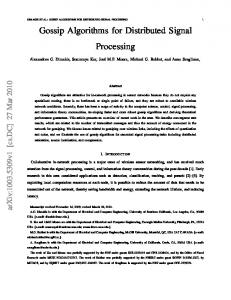
Semantic proximity for file-sharing Author's personal copy Latency for proximity selection..... 2325

M. Jelasity et al. / Computer Networks 53 (2009) 2321–2339

after 2 cycles

after 3 cycles

after 4 cycles

after 7 cycles

Fig. 3. Illustration of constructing a torus over 50 # 50 ¼ 2500 nodes, starting from a uniform random graph with initial views containing 20 random entries and the parameter values m ¼ 20; w ¼ 10, K ¼ 4.


122

Ranking function ✦

✦

Node descriptors contain attributes of the nodes ✦

A number in a sorting application

✦

The id of a node in a DHT

✦

A semantic description of the node

Example: Sorted “Virtual” Ring ✦

Let the ranking function be defined based on the distance d(a,b)=min(|a-b|, 2t-|a-b|) assuming that attributes are included in [0,2t[


123

Ranking function ✦

✦

✦

Node descriptors contain attributes of the nodes ✦

A number in a sorting application

✦

The id of a node in a DHT

✦

A semantic description of the node

The ranking function may be based on a distance over a space ✦

Space: set of possible descriptor values

✦

Distance: a metric d(x,y) over the space

✦

The ranking function of node x is defined over the distance from node x

getPeer(), prepareMsg() are based on a ranking function defined over node descriptors


124




Passive thread




125

Gossip customization for topology construction ✦

✦

local state ✦

partial view, initialized randomly based on Newscast

✦

the view grows whenever a message is received

getPeer(): ✦

✦

✦

randomly select a peer q from the r nodes in my view that are closest to p in terms of distance

prepareMsg(): ✦

send to q the r nodes in local view that are closest to q

✦

q responds with the r nodes in its view that are closest to p

update(): ✦

both p and q merge the received nodes to their view


126

T-man: Topology Management

175 20 90 130 499 700 993


127


175

130 20

10

90

15

130

170

499


getPeer

187

700

800

993

900

128


175

130 20 90


170

130

187

200

Exchange of partial views

10 15

90

170

200

187

700

800

993

900

129


175

130 20

Both sides apply

90

update

130 170 187 200


10 15 90

thereby

170

redefining

187

topology

200

700

800

993

900

130

Distance functions ✦

✦

Example: Line or ring ✦

Space: [0, 1[

✦

Distance over the line: d(a,b) = | a-b |

✦

Distance over thr ring: d(a,b) = min { | a-b | , 1-|a-b| }

Example: Grid or torus (Manhattan Distance) ✦

Space: [0, 1[ · [0, 1[

✦

Distance: d(a,b) = | ax – bx | + | ay – by |


131

Example: Line


132

Sorted Line / Ring ✦

✦

Directional ranking function over the ring defined as follows: ✦

Distance function, line: d(a,b)=|a-b|

✦

Distance function, ring: d(a,b)=min(|a-b|, 1-|a-b|)

Given a collection (view) of nodes and a node x, return ✦

the r/2 nodes “smaller” than x that are closest to x

✦

the r/2 nodes “larger” than x that are closest to x


133

Sorted Line


134

Sorted Ring

0

2m-1

0

2m-1

p

q


135

Sorted Ring

0

2m-1

0

2m-1

p

q


136

T-Man: The movie!

Nodes: 1000 Showing 1 successor, 1 predecessor


Cycles

Nodes

137

Start / stop ✦

✦

In the previous animation ✦

Nodes starts simultaneously

✦

Convergence is measured globally

In reality ✦

We must start the protocol at all nodes ✦

✦

Broadcasting, using the random topology obtained through the peer sampling services

We must stop the protocol ✦

✦


Local condition: when a node does not observe any view change for a predefined period, it stops Idle: number of cycles without variations

138

Fig. 12. Quality of the target TREE graph at termination time as a function ofStart didle ./ stop

size=210 size=213 size=216

active nodes (%)

100 80 60 40 20 0 © Alberto Montresor

0

5

10

15

Time (s)

20

25

30 139

reach all nodes and activate the protocol; almost no delay

T-Man: Scalability

Convergence Time (s)

30 25 20 15 10 5


Anti-Entropy (Push) Anti-Entropy (Push-Pull) Flooding Synchronous start

210

211

212

213

214

215

Network Size (a) SORTED RING

216

217

218 140

The results discussed so far were obtained in static networks, without considering any form of failure. Here, we T-Man: Message costs

Termination Time (cycles)

60 50 40 30 20 10


5

10

15

20

Message Size

25

30 141

T-Man: Robustness to crashes 2335

r Networks 53 (2009) 2321–2339

Target Links Found (%)

100

99.5

99

98.5

98

size=216 13 size=2 10 size=2

0

0.002

0.004

0.006

0.008

0.01

Node failures per node per second © Alberto Montresor

(a) SORTED RING

142

T-Man: Robustness to message losses

M. Jelasity et al. / Computer Netwo

Target Links Found (%)

100 99.8 99.6 99.4 99.2 99 size = 210 13 size = 216 size = 2

98.8 98.6


0

5

10

Message loss (%)

15

20 143

T-Chord ✦

✦

How it works? ✦

Node descriptor contains node ID in a [0..2t[ space

✦

Nodes are sorted over the ring defined by IDs

✦

Final output is the Chord ring

✦

As by-product, many other nodes are discovered

Example: ✦

t=32, size=214, msg size=20


144

T-Chord

5 800

w

Latency (ms)

700

T

600 500 400 300 200


w id lo f f in c r

Chord T-Chord T-Chord-Prox 2

10

2

11

2

12

2

13

14

2 Size

2

15

2

16

2

17

2

18

Figure 4. Message delay as a function of net-

s

C

145

g

Robustness to failures


146

Robustness to failures


147

Conclusions 



This mechanism to build Chord is tightly tailored on the particular structure of Chord A more generic approach: 





Define a ranking function where nodes have a preference for successors and predecessors AND fingers Approx. same results, only slightly more complex to explain

Can be used for Pastry, for example: 


Define a ranking function where nodes have a preference for successors and predecessors AND nodes in the prefix-based routing table

148

Size estimation ✦

Bibliography ✦

A. Montresor and A. Ghodsi. Towards robust peer counting. In Proc. of the 9th Int. Conference on Peer-to-Peer (P2P'09), pages 143-146, Seattle, WA, September 2009


149

Network size estimation at runtime ✦

Why ✦

✦

f(n) routing pointers ✦

to bound the hop count

✦

to provide churn resilience

build group of size f(n) ✦

✦

f(n) messages ✦

✦

Slicing to reduce overhead in gossip protocols

How ✦

Combine and improve existing protocols

✦

Compared to existing systems: ✦

✦

More precise, more robust, slightly more overhead

Simple idea → short paper


150

A brief explanation ✦

Assign random numbers in [0, d[ ✦

✦

Build a ring topology ✦

✦

✦

Locally

Compute the average distance a ✦

127

Gossip topology construction (T-Man)

Compute the distance to the successor ✦

✦

Locally; here, d=127

Gossip aggregation

112

15

15 97 17 80

7 8

14 7

9

23

11.63 16

128/11.63=12

3

10 70

24

4 46

39 42

Compute size ✦

d/a=n


151


Scalability 75 70 65 60 55 50 45 40 35 30

Overhead per node (kB)

5.0 4.0

T-Size Average

T-Size Average

3.0 2.0 1.0 0.0 2


10

2

11

2

12

2

13

14

2 Size

2

15

2

16

2

17

2

18

152

100 10-1 10-2 10-3 10-4 10-5 10-6

10-3

Fig. 2. 10-1


10-4

10-5 10-6 Precision

10-7

10-8

Evaluation of parameter precision.

Error of max estimate

120

153

)

Error (%)

120 110 100 90 80 70 60 50 40

Error of max estimate Error of min estimates Convergence time


Accuracy – w.r.t. parameter Precision

Robustness

103 2

10 Error (%)

1

10

100 -1

10

10-2 -3

T-Size Average

10

10-4

0

0.2

0.4

0.6

0.8

1

Failure probability per second per node (%)

Fig. 6. 100 © Alberto Montresor

T-Size Average

Accuracy under churn.

154

Absolute slicing ✦

Bibliography ✦

A. Montresor and R. Zandonati. Absolute slicing in peer-to-peer systems. In Proc. of the 5th International Workshop on Hot Topics in Peer-to-Peer Systems (HotP2P'08), Miami, FL, USA, April 2008.


155

Introduction ✦

System model ✦

✦

✦

Potentially owned/controlled by a single organization that deploys massive services on them

Examples ✦

✦

✦

An huge collection of networked nodes (resource pool)

ISPs that place smart modems / set-top boxes at their customers' homes BT, France Telecom

Note: similar to current P2P systems, but with some peculiar differences


156

Introduction: possible scenarios ✦

Multiple-services architecture ✦

✦

On-demand services ✦

✦

Nodes must be able to host a large number of services, potentially executed by thirdparty entities

A subset of the nodes can be leased temporally and quickly organized into an overlay network

Adaptive resource management ✦

Resource assignments of long-lived services could be adapted based on QoS requirements and changes in the environment


157

Overview ✦

✦

What we need to realize those scenarios? ✦

Maintain a dynamic membership of the network (peer sampling)

✦

Dynamically allocate subset of nodes to applications (slicing)

✦

Start overlays from scratch (bootstrap)

✦

Deploy applications on overlays (broadcast)

✦

Monitor applications (aggregation)

This while dealing with massive dynamism ✦

Catastrophic failures

✦

Variations in QoS requirements (flash crowds)


158

Architecture: a decentralized OS

Applications

Other middleware services (DHTs, indexing, publish-subscribe, etc.)

Slicing Service

Topology Bootstrap

Monitoring Service

Broadcast

Peer sampling service


159

The problem ✦

Distributed Slicing ✦

✦

Ordered Slicing (Fernandez et al., 2007) ✦

✦

Return top k% nodes based on some attribute ranking

Absolute slicing ✦

✦

Given a distributed collection of nodes, we want to allocate a subset (“slice”) of them to a specific application, by selecting those that satisfy a given condition over group or node attributes

Return k nodes and maintain such allocation in spite of churn

Cumulative slicing ✦

Return nodes whose attribute total sum correspond to a target value


160

Problem definition ✦

We considere a dynamic collection N of nodes

✦

Each node ni ∈N is provided with an attribute function ✦

✦

Slice S(c,s): a dynamic subset of N such that ✦

✦

✦

fi: A → V

c is a first-order-logic condition defined over attribute names and values, identifying the potential member of the slice s is the desired slice size

Slice quality:

|S(c, s)| − s s


161

Problem definition

S

Slice nodes (total slice size ~ s) P

Potential nodes (each node satisfying c)

N


Total nodes

162

Issues ✦

✦

What we mean with “return a slice”? ✦

We cannot provide each node with a complete view of large scale subset

✦

Slice composition may continuously change due to churn

How we compute the slice size? ✦

✦

without a central service that does the counting?

How do we inform nodes about the current slice definition? ✦

Multiple slices, over different conditions, with potentially changing slice sizes


163

Gossip to the rescue ✦

Turns out that all services listed so far can be implemented using a gossip approach ✦

✦

Peer sampling: continuously provides uniform random samples over a dynamic large collection of nodes ✦

random samples can be used to build other gossip protocols

✦

side-effect: strongly connected random graph

Aggregation: compute aggregate information (average, sum, total size, etc.) over large collection of nodes ✦

✦

✦

we are interested in size estimation

Broadcast: disseminate information

Gossip beyond dissemination ✦

Information is not simply exchanged, but also manipulated


164

Architecture of the absolute slicing protocol

Application Protocol Aggregation

S Peer Sampling

Aggregation

P Peer Sampling

Broadcast

N Peer Sampling


165

The slicing algorithm ✦

Total group ✦

✦

All nodes participate in the peer sampling protocol to maintain the total group

Potential group ✦

Nodes that satisfy the condition c join the potential group peer sampling ✦

✦

Means: inject their identifier into message exchanged at the 2nd peer sampling layer

Aggregation ✦

Estimate the size of the potential group size(P)


166

The slicing algorithm ✦

Slice group ✦

Nodes that “believe to belong” to the slice join the slice peer sampling ✦

✦

Aggregation ✦

✦

Means: inject their identifier into messages exchanged at the 3rd peer sampling layer

Estimate the size of the slice size(S)

Nodes “believe to belong” or not to the slice ✦

join the slice with prob. (s-size(S)) / (size(P)-size(S))

✦

leave the slice with prob. (size(S)-s) / size(S)


167

Experimental results: actual slice size


168

Experimental results: churn 10-4 nodes/s


169

Experimental results: variable churn


170

Experimental results: message losses


171

Slicing - conclusion ✦

✦

✦

Absolute slicing protocol ✦

Extremely robust (high level of churn, message losses)

✦

Low cost (several layers, but each requiring few bytes per sec)

✦

Large precision

The message ✦

Gossip can solve many problems in a robust way

✦

Customizable to many needs

What's next? ✦

Cumulative slicing: ✦


very similar, but it's a knapsack problem

172

Function optimization ✦

Bibliography ✦

✦

M. Biazzini, A. Montresor, and M. Brunato. Towards a decentralized architecture for optimization. In Proc. of the 22nd IEEE International Parallel and Distributed Processing Symposium (IPDPS'08), Miami, FL, USA, April 2008.


✦

B. Bánhelyi, M. Biazzini, A. Montresor, and M. Jelasity. Peer-to-peer optimization in large unreliable networks with branch-and-bound and particle swarms. In Applications of Evolutionary Computing, Lecture Notes in Computer Science, pages 87-92. Springer, Jul 2009. M. Biazzini, B. Bánhelyi, A. Montresor, and M. Jelasity. Distributed hyper-heuristics for real parameter optimization. In Proceedings of the 11th Genetic and Evolutionary Computation Conference (GECCO'09), pages 1339-1346, Montreal, Québec, Canada, July 2009.


173

Particle swarm optimization ✦

✦

Input: ✦

A multi-dimensional function

✦

A multi-dimensional space to be inspected

Output: ✦

✦

The point where the minimum is located, together with its value

Approximation problem


174


A solver is a swarm of particles spread in the domain of the objective function

✦

Particles evaluate the objective function in a point p, looking for the minimum

✦

Each particle knows the best points

✦

✦

found by itself (bp)

✦

found by someone in the swarm (bg)

Each particle updates its position p as follows: ✦

v = v + c1 * rand() * (bp - p) + c2 * rand() * (bg - p)

✦

p=p+v


175


Modular architecture for distributed optimization:

✦

The topology service (NEWSCAST) ✦

✦

✦

creates and maintains an overlay topology

The function optimization service (D-PSO) ✦

evaluates the function over a set of points

✦

Local/remote history driven choices

The coordination service (gossip algorithm) ✦

determines the selection of points to be evaluated

✦

spread information about the global optimum


176


Communication failures are harmless ✦

✦

Losses of messages just slow down the spreading of (correct) information

Churning is inoffensive ✦

Nodes can join and leave arbitrarily and this does not affect the consistency of the overall computation


177

Scalability


178

Gossip Lego, reloaded ✦

The baseplate ✦

✦

✦

Peer sampling

The bricks ✦

Slicing (group management)

✦

Topology bootstrap

✦

Aggregation (monitoring)

✦

Load balancing (based on aggregation)

Applications ✦

Function optimization

✦

P2P video streaming

✦

Social networking


179

Conclusions ✦

We only started to discover the power of gossip ✦

✦

✦

Many other problems can be solved

The right tool for ✦

large-scale

✦

dynamic systems

Caveat emptor: security ✦

We only started to consider the problems related to security in open systems


180

Shameless advertisement ✦

PeerSim - A peer-to-peer simulator ✦

✦

Written in Java

✦

Specialized for epidemic protocols

✦

Configurations based on textual file

✦

Light and fast core

Some statistics ✦

15.000+ downloads

PeerSim: A Peer-to-Peer Simulator [Introduction] [People] [Download] [Documentation] [Publications] [Peersim Extras] [Additional Code]

Introduction

Peer-to-peer systems can be of a very large scale such as millions of nodes, which typically join and leave continously. These properties are very challenging to deal with. Evaluating a new protocol in a real environment, especially in its early stages of development, is not feasible. PeerSim has been developed with extreme scalability and support for dynamicity in mind. We use it in our everyday research and chose to release it to the public under the GPL open source license. It is written in Java and it is composed of two simulation engines, a simplified (cycle-based) one and and event driven one. The engines are supported by many simple, extendable, and pluggable components, with a flexible configuration mechanism. The cycle-based engine, to allow for scalability, uses some simplifying assumptions, such as ignoring the details of the transport layer in the communication protocol stack. The event-based engine is less efficient but more realistic. Among other things, it supports transport layer simulation as well. In addition, cycle-based protocols can be run by the event-based engine too. PeerSim started under EU projects BISON and DELIS DELIS. The PeerSim development in Trento (Alberto Montresor, Gian Paolo Jesi) is now partially supported by the Napa-Wine project.

People

✦

150+ papers written with PeerSim

top

top

The main developers of PeerSim are: Márk Jelasity, Alberto Montresor, Gian Paolo Jesi, Spyros Voulgaris Other contributors and testers (in alphabetical order): Stefano Arteconi David Hales Andrea Marcozzi Fabio Picconi


181

Thanks ✦

My co-authors: ✦

✦

For some slides: ✦

✦

Spyros

Those who invited me: ✦

✦

Mark, Ozalp, Gian Paolo, Marco, Roberto, Ali, Maarten, Mauro, Balazs

Marinho, Luciano and Lisandro

And finally: ✦

You for listening!


182

Gossip protocols for large-scale distributed systems - SBRC'2010

Gossip protocols for large-scale distributed systems - SBRC'2010

Suggest Documents

Gossip protocols for large-scale distributed systems - SBRC'2010

Peer-to-Peer Systems and Gossip Protocols

Peer-to-Peer Systems and Gossip Protocols

Gossip algorithms for distributed ranking - Automatica - Unipd

Gossip Algorithms for Distributed Signal Processing - arXiv

Gossip algorithms for simultaneous distributed ... - Automatica

Gossip algorithms for simultaneous distributed ... - Automatica - Unipd

Metaobject Protocols For Distributed Programming

Gossip-Based Broadcast - Distributed Systems Group - INESC-ID

Distributed Synchronization Protocols for SDH

Network access protocols for real-time distributed control systems

An Analysis of Some Delegation Protocols for Distributed Systems

Convergence Analysis of Scalable Gossip Protocols - Electrical ...

Decentralized K-means using randomized Gossip protocols for ... - Hal

Semantic Analysis of Gossip Protocols for Wireless Sensor Networks

CLON: Overlay Networks and Gossip Protocols for Cloud ... - GSD

Gossip-Style Failure Detection and Distributed ...

Efficient gossip and robust distributed computation - Computer ...

GOSSIP: Gossip Over Storage Systems Is Practical - SODA

Location-Aware Cache-Coherence Protocols for Distributed

Network access protocols for real-time distributed

HySoN: A Distributed Agent Gossip Protocol for ... - Semantic Scholar

Gossip-based computation of a Gaussian mixture model for distributed

HySoN: A Distributed Agent Gossip Protocol for ... - Semantic Scholar