Grant Number NAG8-093 An Intelligent Allocation Algorithm For ...

Grant Number NAG8-093

An Intelligent Allocation Algorithm For Parallel Processing

Chester C. Carroll Cudworth Professor of Computer Architecture Abdollah Homaifar Temporary Visiting Assistant Professor of Electrical Engineering and Kishan G. Ananthram Graduate Research Assistant

Prepared for

The National Aeronautics and Space Administration

Bureau of Engineering Research The University of Alabama January 1988

BER Report No. 416-17

ABSTRACT

This research considers the problem of allocating nodes of a program graph, to processors, in a parallel processing architecture. The algorithm is based on critical path analysis, some allocation heuristics, and the execution granularity of nodes in a program graph. These factors, and the structure of interprocessor communication. network, influence the allocation.

To achieve realistic estimations of

the execution durations of allocations, the algorithm considers the fact that nodes in a program graph have to comtnunicate through varying numbers of tokens.

Coarse and fine granularities have been implemented,

with interprocessor token-comanmication duration, varying from zero up to values comparable with the execution durations of individual nodes.

The effect on allocation, of communication network structures, is demonstrated by performing allocations for crossbar (non-blocking) and star (blocking) networks.

The algorithm assumes the availability of as

many processors as it needs for the optimal allocation of any program graph.

Hence, the focus of allocation has been on varying

token-communication durations rather than varying the number of processors.

The algorithm always utilizes as many processors as

necessary for the optimal allocation of any program graph, depending upon granularity and characteristics of the interprocessor communication network.

ii

ACKNOWLEDGEMENT This research was supported by NASA, George C. Marshall Space Flight Center, Huntsville, Alabama, under Grant Number NAG8-093 and conducted in the Computer Architecture Research Laboratory in the College of Engineering at The University of Alabama.

iii

TABLE OF Page ACKNOWLEDGEMENT

iii

LIST OF TABLES

V

LIST OF FIGURES

vii

1

CHAPTW 1 PROBLEM STATEMENT 1.1 1.2 CHAPTER2 2.1 2.2 2.3 2.4 2.5 2.6 2.7

CHAPTER 3 3.1 3.2 3.3 3.4

CHAF'TW 4

1 5

Introduction Literature Review

7

ALGORITHM Introduction Criteria Brief Outline Assumptions Inputs Detailed Description Outputs

7 8

13 14 15 16 29 30

EXAMPLES

30 31 39 46

Introduction Example la Example lb Example 2 RESULTS AND CONCLUSIONS

56 59

BIBLIOGRAPHY

APPENDIX A Pre-allocation analysis and allocation tables for a

61

missile guidance problem

APPENDIX B Determination of earliest times of nodes

65

APPENDIX C Determination of latest times of nodes

66

APPENDIX D Program listing

67

iv

LIST OF TABLES

Page

Table 1

Pre-allocation analysis with equal durations for figure 13

36

2

Resource aIIocation for table I when CT = 0

37

3

Resource allocation for table 1 when CT

37

4

Schedule of interprocessor communication for table 1 when CT = t/2

35

5

Resource allocation for table 1 when C T = t

35

6

Schedule of interprocessor communication for table 1 when CT = t

39

7

Pre-allocation analysis with unequal durations for figure 13

44

8

Resource allocation for table 7 when CT = 0

44

9

Resource allocation for table 7 when C T = t/2

10

Schedule of interprocessor communication for table 7 when CT = tj2

44

11

Resource allocation for table 7 when CT = t

45

12

Schedule of interprocessor communication for table 7 when CT = t

46

13

Pre-allocation analysis for figure 20

53

14

Resource allocation for table 13 when C T = 0

53

15

Resource allocation for table 13 when C T = t/2

54

16

Schedule of interprocessor communication for table 13 when C T = ti2

54

17

Resource allocation for table 13 when CT = t

55

V

=

ti2

.

44

18

Schedule of interprocessor communication for table 13 when CT = t

vi

55

LIST OF FIGURES Page

F-igure

1

A program graph

3

2

Illustration of communication

12

3

Identification of critical paths (case 1)

17

4

Identification of critical paths (case 2)

IS

5

Allocation of node ‘N’ to a parent processor

21

6

Execution and communication durations of parent nodes

23

7

Illustration of earliest executable time

23

8

Illustration of allocation

24

9

Illustration of output priorities

25

10

Slack durations of nodes

26

I1

Illustration of input to critical nodes

26

12

Illustration of input schedules

25

13

Program graph 1

34

14

Timing diagram of graph represented by table 1 for CT = 0

35

15

Timing diagram of graph represented by table 1 for CT

35

16

Timing diagram of graph represented by table 1 for CT = t

36

17

Timing diagram of graph represented by table 7 for CT = 0

42

1s

Timing diagram of graph represented by table 7 for CT

42

19

Timing diagram of graph represented by table 7 for CT = t

43

20

Program graph 2

50 vii

=

=

ti2

t,2

21

Timing diagram of graph represented by table 13 for CT = 0

51

22

Timing diagram of graph represented by table 13 for CT = ti2

51

23

Timing diagram of graph represented by table 13 for CT = t

52

viii

CHAPTER ONE PROBLEM STATEMENT

1.1 INTRODUCTION

With upper limits being reached in the speed of semiconductor technology, new avenues have to be exploited for achieving real time response to many practical problems. Parallel processing promises considerable insight into solutions for such applications. Extensive research is being conducted in this direction. Parallel processing is possible because of the existence of implicit parallel executions of the instructions and tasks of application algorithms. The conventional Von-Neumann architecture employs program control to execute instructions sequentially. Parallel processing utilizes two or more processors connected by a communication network, and, each of these processors may work simultaneously on non data-dependent sub-functions of the algorithms

to achieve faster execution. A parallel architecture may consist of a number of processors, and each of these may execute sequentially under program control or be totally data driven. In either case, the ultimate goal is to achieve a real time response by assigning concurrently executable instructions to different processors. As the cost of hardware is reducing day-by-day, parallel processing

architectures with large numbers of processing elements and various communication networks are becoming viable. These architectures ha\-e sufficient processing power to execute programs for real time systems. Therefore, 1

2

proper utilization of these resources, and intelligent division of the work load between processors could achieve extremely fast algorithm executions. This is precisely the thesis of this research. Any program, or task, may be represented by a program graph. As shown

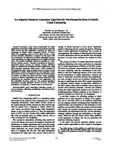
in figure 1, a program graph consists of nodes representing instructions, and connection arcs for the data-dependency between nodes. The parent nodes of any node are those which supply data to it. Similarly, dependents of a node are those to which it supplies data. A node is ready for execution only after its parents have completcd execution, and their results have reached the node. The time expcnded in cxccuting the instruction represented by a node, is the execution duration of the node, while time expended in communicating the result to the node’s dependents, is the communication time. Data is passed between nodes in the form of tokens. Multiple tokens may be required to represent the result produced by any node. Instructions represented by nodes in a program graph determine its granularity, and this increases with the complexity of the nodes. When nodes represent entire functions, the graph is said to be coarsely granular. On the other extreme, if individual nodes represent single instructions, the graph is finely granular. For the propcr utilization of hardware resources to get the

fastest execution; granularity, parallclism, and communication, must all be considered. Conversion of a source program written in an application language, to a program graph, is donc by a compiler. Providcd the problem is similarly coded, the graph gcneratcd by the compilation of different languages would be similar

for a givcn architecture. This is analogous to thc situation whcrc compiled codes

3

of a problem written in different high-level languages are the same for a given uniprocessor.

Figure 1. A program graph

In the case of a uniprocessor system, all instructions are allocated to it. However, in a parallel processing environment, the instructions have to be allocated judicipusly to all the available processors for parallel execution, so that the application program is executed within the minimum amount of time. This

important function of partitioning a program graph and allocation of its nodes to different processors, with a view of obtaining fast execution, is done by an allocation algorithm. The total execution duration of any program graph, in a parallel processing environment, can be subdivided into the actual execution duration of nodes. and the time spent in internode communication. It is the function of the algorithm to minimize the sum of these two durations. In order to minimize the actual

3

execution duration of the nodes, they are to be allocated to different processors,

so that executable nodes do not have to wait for the allocated processor to complete its previous execution. This, however, results in increased internode communication duration, as only communication between nodes allocated to the same processor involves zero time duration. Minimization of internode zommunication duration requires the allocation of all nodes to a single processor, since interprocessor communication involves a finite time as opposed to intraprocessor communication which does not expend any time. This extreme, however, maximizes queueing delay, thereby maximizing the actual time duration

of execution of nodes. A balance therefore, has to be drawn between minimization of queueing and

interprocessor communication delays. Thus, only an optimal amount of parallelism has to be exploited by the algorithm. Factors such as execution speed

of the hardware, bandwidth of the network and granularity of the graph, a11 affect the amount of parallelism that should be exploited for an optimal allocation. An allocation

slgorithm may either be static or dynamic, depending upon

whether it makes allocations prior to, or during run time of the application program. Both methods have their own advantages and disadvantages. A properly designed dynamic allocator may perform better, especially in problems involving inputs from the external world. Since the allocator uses dynamically updated global information of all processors, a more efficient allocation is made. However, communication of the status of individual processors to the allocator may take a large share of the network bandwidth. If sufficient information is not dynamically supplied to such an allocator, it may lead to a bottleneck. The

5

advantage of a static allocation algorithm is that it does not contribute to the actual run time of the application program. Well designed static allocators may be nearly optimal. It should be noted that the problem of allocation is NP-complete. The goal of any allocation algorithm is to minimize run time of the application program. This is attained by minimization of the actual time-of-execution of nodes, interprocessor communication time and run time analysis of the graph.

1.2 LITERATURE REVIEW

This research includes a discussion of some algorithms that have been developed by researchers, in an effort to find a near optimal solution to the NP-complete problem of allocation. Some of these algorithms have been directed at specific architectures and applications. Although, tho houristics on the basis

of which these algorithms have been developed are different, all of them aim at the realization of real time response. Hong, Payne and Ferguson [ 11 have developed a n algorithm for dynamic

hypercube architectures. Their scheme divides the original program graph into disjoint tree shaped partitions. Nodes of some of these trees have only one input, while those of others have only one output. Individual trees are then mappod onto distinct faces of the hypercube. Every node in a tree is allocated to a distinct processor, located as close as possible to the processor which computes its parent. Campbell [2] proposed a static allocation algorithm for 3-Dbussed cube architectures. His algorithm consists of local and global allocators. After topologically sorting the nodes in a breadth-first manner, thc local allocator

6

assigns them to individual processing elements of the Hughes dataflow machine.

In selecting a suitable processor for any node, the allocator applies two heuristic cost functions, namely, parallel processing cost and communication cost; and allocates the node to the processor returning the lowest total cost. The global allocator is similar to the local allocator, but only works on larger parallel modules consisting of several nodes, and allocates each of these modules to different sections of the hardware. Due to the amount of computation involved

in allocating each node, this algorithm takes a long time to arrive at an optimal result. Ho and Irani [3] proposed a static allocation algorithm which simulates runtime environment. Their scheme requires much information about the changing environment. For any node, this algorithm selects the processor which gives the best performance in simulation. As this algorithm also involves estensive computation, it is a lengthy process.

For graphs which are not so finely parallel, a lot of scheduling algorithms have been developed. While some of these algorithms totally neglect interprocessor communication time. others try to avoid it by redundant execution

of nodes on various processors. Markenscoff and Liaw [4] have developed allocation schemes for distributed systems. Their schemes, namely, branch and bound, greedy and local search, do not allow interprocessor communication. Hence, nodes upon which any node is dependent for its input data, also have to be allocated to the same processor. This results in redundant execution of many nodes. The tradeoff in this case is between redundancy in execution and interprocessor communication time.

CHAPTER TWO ALGORITHM

2.1 INTRODUCTION As mentioned in the earlier chapter, an allocation algorithm is crucial to the

exploitation of parallelism in a program graph and the proper utilization of hardware resources. An efficient, optimal map of nodes to processing elements, is obtained only when parallelism and sequentialism in the program graph, execution durations of the various instructions, and interprocessor communication durations are all viewed in the proper perspective. Only an algorithm which considers all these important factors arrives at a practical map, and makes a realistic .estimate of the duration of execution. Time taken in interprocessor communication has not been given sufficient importance in some of the allocation schemes described earlier. Communication between processors involves a certain finite time due to transmission of data tokens. Only in graphs whose nodes are of coarse granularity, wherein the execution time of any node is much larger than the commmunication time, can the latter be totally neglected. The significance of interprocessor comnunication time delay increases as its ratio with execution time increases. This is of prime importance when communication time is comparable with execution time. Due to this communication delay, even an optimally allocated graph may not execute within the minimum time as dictated by its critical path (to be discussed in the 7

8

foIlowing section). Hence, interprocessor communication time has to be given due importance while allocating a program graph. It may be necessary to sacrifice a certain amount of parallelism due to the interprocessor communication involved.

2.2 CRITERIA

Certain factors are important to an allocation algorithm. These are earliest time, latest time, critical paths, network characteristics, processor execution and communication characteristics, etc. Nodes in a program graph can be executed only when they have received their individual inputs. Thus, the earliest that a node is executable is when all of its parents have completed execution and the results have been passed on to the node. A term called 'earliest time of the node' follows from this. The earliest time of a node specifies the earliest that the node may begin execution, and is determined by the input that arrives 1 s t (deterministic input). It depends upon execution time durations of previous nodes, and is defined as being equal to the time at which all inputs to the node are available, provided that all the previous nodcs have executed at their respective earliest times. It may also be defined as the maximum of the sum of earliest times of parent nodes and their respective execution time durations. The earliest time of a node with no parents is equal to zero. The algorithm represented in appendix B uses the latter definition to detcrmine earliest times of nodes in a program graph. When all nodes in a program graph execute at their carlicst times, the graph

is executed in the minimum possiblc timc duration. This timc duration is callcd thc 'minimum time of execution.' It is not possible to excmte 3 p p h within a timc frame lcss than thc minimum timc of cxccution. An zr1location that achicvcs

9

execution in the minimum time of execution is the optimal one. Thus, the minimum time of execution gives a theoretical lower bound for the execution duration of the graph, and is a good measure for evaluating the performance of an allocation algorithm. I t is to be mentioned here that the definition of minimum time of execution assumes zero communication delay between nodes. Hence, in practical systems, in which interprocessor communication has a finite significant value, it is not possible to make an allocation that will execute the graph within this time frame. The earliest time of a node, which was defined earlier, is the time at which all the inputs to the node are available, provided parcnt nodes had executed at their respective earliest times. Thus, the earliest time of any node is determined by the input that arrives last. The other inputs may arrive at any time prior to the arrival of the deterministic input. Those parents which are the sources of thcse non-deterministic inputs may execute at a time later than their earliest times, and the program graph could still execute within the minimum time of execution. This leads to the definition of another term called the ‘latest time’. The latest time of a node is the latest it may execute, without prolonging the

execution of a graph, beyond its minimum time of execution. It is hence obvious that the latest time of a node with no dependents, is equal to the difference between the minimum time of execution of the graph and the execution duration of the node. The latest time of any other node is equal to the difference betwccn the minimum of the latest times of its dependents and its execution duration. This definition is implemented in the algorithm shown in appendix C. A node may begin execution any time between its earliest and latest timcs

without increasing the total execution time of the graph. This time period,

10

between the node’s earliest time and latest time, is known as the ’slack’ or the ’optimally enabled state’ of the node. It is highly desirable that every node should begin execution in its slack to achieve minimum time duration of execution of a program graph. The earliest time and latest time of certain nodes are found to be equal. These nodes are called critical nodes, as delaying their execution beyond their earliest times results in an increase in the duration of execution of a graph by an amount equal to the delay. In order to achieve minimum duration of execution, it is very important that these critical nodcs be scheduled for esccution at their

respective earliest times. Non-critical nodes may be scheduled for esecution. any time between their respective earliest and latest times. without sacrificing the speed of execution. Study of many program graphs has revealed that critical nodes occur in sequence thereby forming a critical path that runs through thc program graph. A graph may have one or more such critical paths. Nodcs in a critical path are

not only critical but also sequential. Communication is very important in a parallel procossing cn\.ironment. To

capitalize on gains made by parallel processing, an efficicn t communication network is necessary. The allocation algorithm should schcdule the flow of tokens

so that network contentions do not occur. The characteristics of different networks vary. A star network can be implemented with minimum hardware. however, it allows only one pair of processors connected to it to communicate at a time. The communication distance between any two pairs connected to a star

is a constant. A crossbar network between the processors, would be totally non-blocking, allowing simultaneous communication between processors. E l m

11

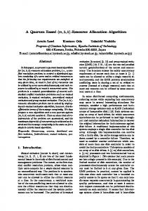
in this case, a processor may not receive information simultaneously from two or more processors. Study of program graphs has revealed that although some nodes within each module can be executed in parallel, communication between nodes can be scheduled sequentially without a great loss of performance. Thus, the allocation algorithm has to schedule transmission of data from one node to another so that network or processor contentions do not occur, and data reaches destination nodes within their slack times. The next factor to be considered is the communication characteristic of individual processors. Usually, processors can either send or receive only one data token at any given time. As mentioned before, many nodes are to be assigned to each processor. Each node assigned to a processor, may send or receive one or more tokens to or from other processors. The allocation algorithm should schedule all communication of this processor so that contention does not occur. Particular attention is to be paid in scheduling communication caused by directly data dependent nodes that are assigned to the same processor. A parent node assigned to a processor will need to communicate its result to all its dependents, while one of its dependents which is assigned to the same processor, may simultaneously need to get its data from its other parents. This situation is illustrated in figure 2. Therefore, the order in which results have to be sent to dependents, and the instants at which these have to be done. is to be intelligcntly decided by the algorithm. Due to the limited instruction storage capacity of each processor, only

8

certain number of nodes can be stored at any given time. Likewise, the number

of nodes that the architecture can hold at any given time is also limited. If thc number of nodes in a program graph is greater than the storage capacity of the

,

architecture, or even if more nodes than can be stored in a processor has to be allocated to it, some nodes will have to be loaded during run time. This can be done in two different ways. In the first method, the allocation algorithm divides the node-to-processor map into many modules, and successively loads these

6 Figure 2. Illustration of comrnunication

modules as each completes execution. Therefore, after execution of each module, 3

certain amount of time is expended in loading the nodes of the next module on

to the processors. This method is especially suited to architectures whose communication networks have small bandwidths. In architectures having more extensive communication structures, a different method may be used. As 3nd when nodes are executed in the processors, they are removed from the instruction store, thus creating free memory space in which new instructions may be loaded.

13

New nodes may therefore be loaded on to the processors by the allocation algorithm, simultaneously with the execution of the program; and for doing this a load time has to be associated with each node. It is at this load time, that the allocation algorithm loads the node on to the processor. This method could be well implemented in a non-blocking communication network architecture, such as a crossbar, and also in blocking networks when the program graph is coarsely granular. Allocation of critical nodes, and the exact scheduling of their execution, is extremely crucial to the execution of a program graph, in the minimum possible time. Similarly, scheduling the execution of non-critical nodes within thcir slack times is also important. I t may not always be possible to do this due to communication characteristics of the architecture, and fineness in the granulririL:. of a program graph. The exact scheduling of critical nodes is attempted by

assigning all the nodes in a critical path to a single processor. In addition to doing this, the inputs to these critical nodes should reach the assigned proct.h.kir prior to their critical times. In allocating non-critical nodes, the algorithm should locate a processor that is idle during the node’s slack period, and allocate the

node to it if all inputs to the node can reach it within its latest time. If one such processor is not available, the algorithm should allocate the node to any other processor, so that delay in execution of the node beyond its slack time is a

minimum.

2.3 BRIEF OUTLINE

The algorithm adopted in this research, involves the determination of critical paths, and-allocation of each critical path to an individual processor. Once the

14

processors for all critical paths are identified, the algorithm then sorts all the nodes in an increasing order of their latest times. Nodes with the same latest times are sorted in a decreasing order of their earliest times, which is the same

as the increasing order of their slack times. Nodes in a program graph are allocated one-by-one as per the order established earlier, on the basis of certain principles that are described in a later section. The various phases in the algorithm are listed below.

-

Ordering the nodes for allocation.

-

Assigning of critical paths to processors.

-

Allocation of nodes to processors, scheduling of their execution and their

Determination of earliest times. Determination of latest times. Determination of critical paths.

communication. The first four, of the above phases. fall into the pre-allocation processing group, while the last two compose the allocation group.

2.3 ASSUMPTIONS Assumptions made in the design of this allocation algorithm are described

in this section. Very large programs are already partitioned, if possible, into smaller modules that have very little, or no data-dependency between them. This may be done by looking at the syntax of the high-level language which is the source

of the program graph. The algorithm works on these modules, one at a time, and maps them on to a hardware submodule (cluster, 9 side of a hypercube, ctc.).

1s

The nodes in each partitioned module of a program graph are numbered by some other algorithm, so that a parent always has a numerically lesser node number than its dependents. The algorithm assumes the availability of an unlimited number of processing elements on to which it can allocate the program graph. This is justifiable as hardware cost keeps reducing with advances in technology, and a lot of processing elements may be used in any architecture. Hence, the graph may be spread in an optimally parallel fashion without any loss of parallelism due to hardware constraints. The algorithm needs as its input, and hence assumes the availability of time durations of execution of various instructions that are associated with the nodes

in a program graph. It is possible to determine the execution duration of all the instructions of a processor. Another input needed by the algorithm, is a list of communication time durations for a single token between various processors in an architecture. Interprocessor communication time durations depend upon the structure of the interconnecting network between processors in a module of the hardware

archi tect ure. Communication between processors is by token passing. The outputs produced by different nodes may be of varying lengths, and hence require different numbers of tokens.

2.5 INPUTS The inputs to the allocation algorithm are listed below.

-

Table of execution durations of the various instructions.

16

-

Table of interprocessor communication times for a single token.

-

Program graph, with the nodes numbered in an order of dependency.

-

Number of tokens needed to represent the output of each node.

2.6 DETAILED DESCRIPTION As mentioned earlier, the algorithm works in various phases that fall into

two distinct groups. The analysis group comprises of the determination of earliest times, latest times and slack periods of nodes, determination of critical nodes and critical paths, and the ordering of nodes for allocation. The allocation group involves the allocation of critical paths, scheduling execution of nodes and scheduling of interprocessor communication. The earliest times of all nodes are determined by using the algorithm shown

in appendix B. Determination of earliest times begins with node number one, the root node with no parents. Finally. the minimum time of esocution of the program graph is determined. The next phase in the analysis of a program graph, is the determination of !atest times and slack durations of all nodes. The algorithm for this is shown in appendix C. Determination of latest times begins with the final node hac-ing no dependents and the largest node number. The latest time of any node is determined by the least value of the latest times of its dependents. Critical nodes and critical paths are next identified. All nodes having their earliest time equal to their latest time are critical nodes. These nodes have no slack durations, and have to be scheduled for execution exactly at their critical times to avoid lengthening program execution. Critical nodes occur sequentially

in a program graph forming one or more critical paths.

17

Identification of critical paths is done as follows. Any critical node having

no inputs from other critical nodes is considered to head a critical path. If only one parent of a critical node, is critical, the node is identified as belonging to the critical path formed by this parent. In certain cases, two or more parents of a critical node are also critical, and on the basis of certain principles, the critical node has to be identified as belonging to one of the critical paths formed by its parents. Figure 3 illustrates such a case, where both parents of the critical node

N are critical, and only one of these parents is the last node of a critical path (critical path 1 ). The other parent, in critical path 2, already has a critical successor identified with it. In such cases, the node is identified with critical path 1.

Path 2

Critical

Figure 3.

Identification of critical paths (case 1)

In another case, as illustrated by figure 4, both critical parents of the critical node N, are the last nodes in their respective critical paths. In such cases, the node is identified as belonging to the path formed by the parent that completes execution last, and hence determines the critical time of the node. If both parents complete execution at the same time, the node is identified with the path formed by the parent that generates more output data, so that a smaller amount of time

is lost in interprocessor communication. The final phase in the pre-allocation analysis group is the ordering of nodes for allocation. Nodes with lower values of latest times have to be allocated first. Amongst nodes with equal latest times, those with shorter slacks are given priority. To do this, nodes are numbered in an increasing order of their latest times, and those with equal latest times are numbered in a decreasing order of their earliest times.

Critical Path 2

Figure 4. Identification of critical paths (case 2)

19

Critical paths determined earlier are each identified with a processor. The algorithm considers one critical path at a time, and identifies nodes in the path with a single processor free to execute them at their critical times. These nodes are later allocated to the identified processor. As the algorithm assumes the availability of an unlimited number of processing elements, it can be guaranteed that an idle processor will be found for allocation of each critical path. The reason for allocating all nodes in a critical path to a single processor, is they are essentially sequential, and the critical time of any node is exactly at the completion of execution of its parent node in the critical path. Allocation of such data-dependent nodes to different processors would definitely lead to interprocessor communication delay. If on the other hand, these nodes are allocated to the same processor, communication delay is introduced only if data tokens coming from other parents cannot reach the processor within the latest times of the nodcs. Both critical and non-critical nodcs are next allocated sequentially in the order established earlier. Allocation of non-critical nodes in\-olves the determination of a processor that is idle to execute the node during its slack time, and is also free to communicate with the processors that have the node’s parcnts and dependents assigned to them. Determination of a processor for non-critical nodes is carried out by the application of certain principles that are discussed next. It is apparent that any node, and any of its parents, cannot be executed in parallel due to the data dependency between them. The relationship between them is essentially sequential, and the node maybe executed only after the execution of its parents. The parents of a node may however, be executed in parallel and can be allocated

20

to different processors. In order to avoid delay due to interprocessor communication, the node has to be allocated to the same processor as its parent. Figure 5 shows a node N with earliest time En and latest time Ln. Ideally, execution should begin a t a time between En and Ln. In most cases a processor, to which one of the parents Pa, Pb or Pc is assigned, will be free to execute node

N between En and Ln. The node N is then allocated to this processor. In case two or more processors which have parents assigned to them, are free to execute node N some time between En and Ln, an intelligent selection has to be made. I t is assumed that ta, tb and tc are the beginning times of execution, and d,, d b

and dc, are the durations of execution and a, b and c are the number of tokens in the result of parent nodes Pa, Pb and Pc respectively. If either a, b or c is unusually large (result being large, such as a string), then node N is allocated to corresponding processors PRa, PRb or PRc respectively. This eliminates exccssive communication, and hence reduces network or processor contentions. If a, b and c are all comparable, then node N is allocated to the parent processor

(proccssor to which one of the parent nodes is allocated) that returns the highest value for the expression given below. tx

where x

=

+

dx

+ x*k

(1)

a, b, c and k = time duration of communication of one token.

In the event that none of the parent processors PR,, PRb, PRc etc. are free to execute N in its slack period, any processor (including parent processors) that returns the minimum value for the expression given below is selected. Executable time

=

MAX (X,Y)

(2)

where X is the time at which all tokens arrive from the parent processors, and Y

is the earliest the proccssor is free to execute the node.

21

The assumption of the availability of an unlimited number of processors, assures that a free non-parent processor can be found to execute the node at any time. If the time at which data can be sent to this processor, from the node's parents, is less than executable times of the parent processors, the node is allocated to it; else it is allocated to the parent that is free earlier. I t then incurs queueing delay. Hence, a tradeoff is made between queueing delay and communication delay.

IPR,

IPR,

b-b--

Figure 5. Allocation of node 'N' to a parent processor

Figure 6 shows an application of the principle mentioned earlier. The node

N is allocated to PRb so that communication between node Pb and N does not have any effect. The time tn at which the node may begin execution is when its other inputs from Pa and Pc have reached Pb. As a processor can receive information from only one processor at a time, communications from Pa and Pc to PRb, have to be done sequentially. This is

'

22

illustrated in figure 7. In this case, tn is the exact time at which node N can execute. If tn lies between En and Ln, or if En and Ln are after tn, then the node

N may be executed without any delay, else an inevitable communication delay is introduced.

In figure 8, parents P i and P2 of N2, have been allocated to processors PR1 and PR2 respectively. The dependents of P i are N1, N2 and N3, and those

of P2 are N2 and N4. The allocation of node N2 is now explained. Supposing the order established in pre-allocation mode returned a higher priority (lower number) for N2, than for N1 and Nf,N2 could be allocated to either P R I or PR2, depending upon which one of them returned a higher value for espression 1. If one of the parent nodes generates comparatively a large amount of data,

N2 is allocated to that parent's processor. On the other hand, if

N? is given a

lower priority than N I and NJ, it cannot be allocated for immediate esccution on either PR1 or PR2, due to N1 and N 1 already being allocated to them. In such an event, the processor that returns a minimum 1,alue for expression 2 is selected. Once a node has been allocated to a processor, communication of outputs from the node have to be scheduled. Tokens have to be sent to the dependents in an increasing order of their latest times. When two or more dependents have the same latest time, output is first sent to the node with a greater number of dependents. In figure 9, output is first'scheduled to node D,.

ccccc 0

PE

t

cccccccccccccccccccc

0

I

pc C

Y

t

Figure 6. Execution and communication durations of parent nodes

I

cc c c

caca

Figure 7. Illustration of earliest executable time

. PR1

Figure 8.

9

P R2

p R3

Illustration of allocation

25

Figure 9. Illustration of output priorities

Another criterion that influences communication scheduling, is the earliest time of dependent nodes. Although it is desirable to have the output routed to dependent nodes just before their earliest times, doing it much earlier to this is not advantageous. In figure 10, although 1, < lb, output from node N may be first routed to dependent Db,if the output to dependent Da can still be routed so that it reaches D, within its slack time. When one or more dependent nodes are critical nodes, the output should first be directed to these nodes without delay. A little delay, even beyond the latest time, can be tolerated by non-critical nodes.

26

DA

0

I

I

I

I

EA

LA

Figure 10. Slack durations of nodes

Figure 11. Illustration of input to critical nodes

t

27

Every time communication is scheduled between two processors due to token passing between nodes allocated to them, it is recorded, so that other communications are not scheduled to the processors at those same time. Therefore, communication durations of all processors, due to data transfer between nodes allocated to them have to be recorded. In blocking communication networks, even various communication durations of the network have to be recorded. Likewise, to avoid scheduling two or more nodes for execution simultaneously on the same processor, execution duration (busy times) of each processor is recorded. The priorities in which outputs of a node are to be sent to its dependents are established immediately after its allocation. However, actual scheduling of these communications can be made only after the dependent nodes are allocated. Thus, when a node is allocated, its inputs are actually scheduled, while its outputs are given priorities. Scheduling of inputs can be done only after all of its cousins (other dependents of its parents) have also been allocated.

.

In figure 12, Pa and Pb are the parents of node N, and nodes C1, C2 and C3 are its cousins. The dependents of Pa are N and C1,and the output from

Pa is prioritizcd as (N, C1 ). The dependents of Pb, and its output priorities are given by (C2, N, C3 ). In this case, the input to N from Pa can be scheduled immediately after its allocation, while its input from Pb has to be scheduled only after the allocation of C2. The algorithm associates certain information with each node. The following information regarding each node is supplied as input to the algorithm. Each node is given a 'node number' for identification. The 'instruction number' associated with it identifies the instruction that the node executes. The 'number of parents',

.

28

their respective node numbers, ’number of dependents’ and their respective node numbers, give the data-dependencies of the node. The ’number of tokens’ needed to represent the output produced by the node is also given as input to the algorithm. The following information associated with each node is generated as output by the algorithm. The ’load time’ specifies the time at which the node is to be sent to the processing element. The ’earliest time’ and ‘latest time’ of the node are determined by the algorithm. The ‘execution time’ specifies the time at which the node is scheduled for execution on its assigned processor. The algorithm also determines the priorities and schedules for communication of results to the node’s dependents.

Figure 12. Illustration of input schedules

The algorithm associates some information with each processor, to aid it in its allocation. The ’number of nodes allocated’ to the processor is always

updated. The ’final ready time’ of the processor, which is the earliest time beyond ~

which no nodes are scheduled for execution on it, aids the algorithm in dlocating

29

subsequent nodes. The time periods during which the processor is busy executing nodes, and the time periods when the processor is communicating with other processors, are also recorded.

2.7 OUTPUTS The outputs of the algorithm are listed below. 1. Processor allocated to each node.

2. Load-time and execution beginning time of each node. 3. Schedules of outputs to dependents, for each node. 4. Busy and communication durations of each processor.

5. Various communication durations of the network.

.

CHAPTER THREE EXAMPLES

3.1 INTRODUCTION

In this chapter, two examples are presented to illustrate the allocation algorithm delineated in chapter 2. Reiterating what was mentioned earlier, it can most definitely be stated that, efficiency of an allocation made by any algorithm ~ 1 be 2

measured by the zroximity between values of actual duration of execution

of a graph, and the minimum time of execution as dictated by the critical paths,

when time taken in interprocessor communication is assumed to be zero. The examples are presented in a form to illustrate node-by-node allocation, and scheduling of communication between nodes. The basic time unit is assumed to be t. In the examples shown, execution duration of various instructions vary from t to 4t. Communication between nodes is by token passing. Depending upon the amount of data to be sent by any

node to its dependents, multiple tokens may be necessary to represent it. For each graph, allocation has been made for different values of communication time (CT) of a single token (for CT = 0, ti2, t). To illustrate the flexibility of the algorithm with respect to the arxhitecture, allocation has been done for both blocking and non-blocking communication networks. When the communication time of a single token is assumed to be zero, a program graph represents a coarse grain system, in which communication time is 30

31

negligible compared to execution time of individual nodes. On the other egtreme, when communication time of a single token is assumed equal to t, the program graph represents a fine grain system in which the flow of information between nodes takes as much time as the execution durations of individual nodes. Thus, the allocations indicate the algorithm’s applicability to different levels of parallelism. Pre-allocation processing, which encompasses the determination of earliest and latest times of all nodes, and the ordering of these nodes for allocation, is not explained in this chapter. Only, identification of critical paths and the actual allocation of nodes are explained.

3.2 EXAMPLE l a The first example is shown in figure 13. In order to clearly illustrate the allocation principles, first, equal esecution durations o f t arc assummed for all nodes. Also, with the same intention, interprocessor communication time is assumed to be zero for this example. Later examples in this chapter take the communication delay into account. Table 1 represents pre-allocation analysis of figure 13, and lists the nodes in the graph, their execution durations, earliest times, latest times, number of tokens and their order of allocation. The minimum time of execution of the graph is found to be St. Nodes 1, 2, 6 , 7 and 9 are identified as critical nodes. When the graph is traversed from node 1 to node 9, all critical nodes are found to be sequential, thereby forming only one critical path. In this graph, there is no instance of a critical node having more than one critical parent. As per the principles of the algorithm, these critical nodes have to be allocated to the same processor, namely processor 1. Their execution times

.

32

are decided after the allocation of their parents. The timing diagram shown in figure 14 represents the allocation of this graph. Nodes are allocated in the order that was established in the pre-allocation mode. Node 1 is scheduled for allocation at time ’0’ on processor 1. Node 2 is scheduled on processor 1 at time t, and node 6 is scheduled on the same processor at time 2t. Node 3 is to be executed between its earliest time t and latest time 2t. As processor 1, to which node 3’s parent, node 1 is allocated, is busy during this time frame, node 3 is scheduled for execution at time t on processor 2. Similarly, node 4 is scheduled

on processor 3 at time t. The critical time of node 7 is 3t, and its parent nodes 6, 3 and 4 have all complete execution by time 3t, hence, node 7 is scheduled for execution on processor 1 at time 3t. Node 5 is to be scheduled between its earliest time 2t and latest time 3t. As processor 1, to which its parent, node 2 is allocated,

is busy during this time frame, node 5 is allocated to processor 2 and scheduled for execution at 2t. Node 8 is scheduled for esccution at its carliest time 3t on processor 3 to which its parent, node 4 is also allocated. The critical node 9 is scheduled for execution on processor 1 at its critical time 4t, as all its parents ha\*e completed execution by this time. As illustrated in figure 14, the graph completes execution by 5t, which is its

minimum time of execution. Three processors have been utilized by the algorithm to schedule the graph’s execution. The allocation for this case is prescnted in table 2, appearing at the end of this section. Timing diagrams of figures 15 and 16, and tables 3 and 5 reprcscnt thc allocation of the graph, when time duration for interprocessor communication of a single token is assumed to be ti2 and t respectively. The respective interprocessor communication schedules are shown in tables 4 and 6. All nodes

33

are assumed to generate only one token as their outputs. Communication of tokens between nodes allocated to the same processor is assumed to involve no time. Due to the structure of the communication network (crossbar), broadcast ability in transmission of tokens to dependents, is made use of. These allocations are not explained here, as a detailed explanation of a more general case involving communication appears at a later stage in this chapter. As illustrated in figure 15, the graph will complete execution within a time

period of 5.5t when token communication duration is tj2 (half the execution duration of any node). This represents an increase of only 0.5t beyond the minimum time of execution of the graph. When token communication duration is assumed to be equal to execution duration of any node, as shown in figure 17,

the graph is scheduled on three processors to execute within a time period of 7t.

Figure 13. Program graph 1

35

PR3

1 I 4 I) 8 ( 1 2 3

I1

I

I i

4

I 1

5

1I

6

1

I

7

8

9

Figure 14. Timing diagram of graph represented by table 1 for CT = 0 I I

'. I

\S

PR3

I 1

% '

Y

4, I

2

14 1

3

1

1

I

I

4

5

I

I

1

I

I 1

1

6

7

8

9

1

Figure 15. Timing diagram of graph represented by table 1 for CT

T

t,:'2

~

36

% '

2

3

4

5

6

7

8

9~

Figure 16. Timing diagram of graph represented by table 1 for CT = t

Table 1 Pre-allocation analysis with equal durations for figure 13

.

37

Table 2 Resource allocation for table 1 when CT = 0 Processor

PRl PR2 PR3

Nodes (x,y,z) ( O,I, t) ( t,2,2t) (2t,6,3t) (3t,7,4t) (4t,9,5t) ( t , 3 m (2t,5,3t) ( t,4,20 (2t,8,30

(x,y,z) : Xode Sy is scheduled to begin execution at x and end at z

Table 3 Resource allocation for table 1 when CT = t.'2

I Processor I PRl PR2 PR3

Sodes (X.Y.Z) ( 0.1, t) ( t,2,2.0t) (2t,6,3t) (3.5t,7,4.5t) (4.5t,9,5.5t)

(1.5t,3,2.5t) (2.5t,5,3.5t) (1.5t,4,2.5t) (2.5t,S,3.5t)

(x,y,z) : Xode Sy is scheduled to begin execution at x and end at z

I

38

Table 4 Schedule of interprocessor communication for table 1 when CT = t/2

I

N1

I

N2

(d,p,x,y) : Communication to dependcnt ’d’ allocated to processor ‘p’ is scheduled between ’x’ and ’y’.

Table 5 Resource allocation for table 1 when CT =

Processor

t

Sodes (x,y,z)

PRl

( O,l, t) ( t,2,2t) (2t,6,3t) (3t,5,4t) (jt,7,6t) (6t,9,7t)

PR2

(2t,3,30 (2t,4,3t) (3t,8,4t)

P.R3

(x,y,t) : Node Ny is scheduled to begin execution at x and end at z

.

39

Table 6 Schedule of interprocessor communication for table 1 when CT = t

(d,p,x,y) : Communication to dependent 'd' allocated to processor 'p' is scheduled between 'x' and 'y'.

3.3 EXAMPLE l b

Table 7 , a pre-allocation analysis table, presents unequal execution durations

for the nodes of the program graph in figure 13. The table also lists the number of tokens necessary to represent the result generated by each node. These are also

assumed to be unequal. The earliest time, latest time and order of allocation of each node, as determined by pre-allocation analysis are also shown in it. Allocation of the graph represented by this table for token communication durations of 0, 0.5t and t are represented by figures 17, 18 and 19, and tables 8, 9 and 1 1 respectively. Interprocessor communication schedules for token communication durations of t/2 and t are represented by tables 10 and 12 respectively. The allocation represented by figure 1S is explained in the following paragraph.

Pre-allocation analysis returns a single critical path formed by nodes 1, 2, 6,

7 and 9. According to the principles of the algorithm, these are to be assigned to a single processor, namely processor 1. Node 1 is scheduled for execution on processor 1 at time zero. Node 2 is scheduled at time 3t on the same processor. The next node scheduled, according to the order determined, is node 4. The earliest and latest times of this node being 3t and 4t respectively, it is desirable that this be scheduled for execution as early as possible after time 3t. Processor 1, to which node 4’s only parent, node 1 is allocated, is busy during its slack.

Hence, node 4 is scheduled on processor 2. As node 1 needs two tokens to represent its output, it takes one time unit to communicate its output to a different processor. Hence, node 4 is scheduled for execution at time 4t on processor 2. Communication between node 1 (allocated to processor 1) and node

4 (allocated to processor 4) is scheduled to occur at 3t, and lasts for a duration o f t . Critical node 6 is scheduled for execution at time 5t on proccssor 1. Like node 4, node 3 is also only dependent upon node 1 for its input. It is similarly allocated to processor 3, and scheduled for execution at time 4t. As the crossbar nctwork allows broadcast communication, data transfer from node 1 , to nodes 3 and 4, is scheduled to occur simultaneously. Critical node 7 is to be executed at time 6t if delay is not to be introduced in the execution of the program sraph. I t needs inputs from nodes 3, 4 and 6. As node 6 is also allocated to processor

1, only inputs from nodes 3 and 4 are to be scheduled. Node 3 completes execution at 5t, and its output is represented by a single token. Hcnce, communication between node 3 and node 7 is scheduled between time 5t and 5 . 3 . Node 4 completes execution at 6t, and its output is represented by two tokens, thus involving a communication duration of t. Communication between nodes 4

41

and 7 is scheduled between 6t and 7t. Thus, the earliest node 7 may execute due to communication involved, is 7t (its critical time is 6t). Node 7 is therefore scheduled for execution at 7t. Next in line for allocation, is node 5. The earliest and latest times of this node are 5t and 9t respectively. Its only parent, namely node 1, has been allocated to processor 1. As the duration of node 5 is t, and processor 1 is free between 6t and 7t, node 5 is scheduled for execution at 6t on processor 1. Node 8 can be executed at any time between 5t and 9t without introducing queueing delay. As node 4, the only parent of node 8, is allocated to processor 2, node S is scheduled for execution processor 2 at time 6t. Critical node 9 is to be scheduled on processor 1. I t needs inputs from nodes 5 , 7 and S. As nodes 5 and 7 are allocated to processor 1, only its input from node S has to

be scheduled. Node 8 completes execution on processor 2 at 7t, and produces

only one token. Thus, the communication between node S and 9 is scheduled between 7t and 7.St. Node 9 is scheduled for esecution on processor 1 at time 1 It, which is the time node 7 completes execution. Thus, the total execution

duration of the graph is found to be 1%. T h e minimum duration of execution of this graph, as obtained by earliest time analysis, was 14t. Allocation of the graph for zero interprocessor token communication delay results in an execution duration of I4t (the minimum value possible). Considering interprocessor token communication duration as 1,2t and t, execution durations of the allocation are found to be 15t and 17t respectively.

O n e observation that can be made from figures IS and 19 is that although all the nodes in a critical path are allocated to the same processor, some of them cannot be executed at their critical times due to their data-dependency on non-critical nodes, and the finite time involved in interprocessor communication.

+-

JN

I

J O

E

Q,

1 0

ar"

a,

,

ruR

a,

OD

43

I

J

d-

Table 7 Pre-allocation analysis with unequal durations for figure 13

6 7 8

4t

9

4t

t

t

I 3 1 2

5t 6t 5t lot

5t

6t 9t 1Ot

4 6 8 9

Table 8 Resource allocation for table 7 when CT = 0 Sodes (x,y,z) ( 0,1,3t) (3t,2,5t) (5t,6,6t) ( 6 ~ 7 , 1 0 0 (10t,9,14t) (3t,-l,5t) (5t,S.6t) (3t,3,5t) (5t,5,6t)

Processor PRI PR2 PR3

(x,y,z) : S o d e Syis scheduled to begin execution at x and end at z

Table 9 Resource allocation for table 7 when CT = t,’2

I

~

Processor I Sodes (x,y,z) PRI (0,1,3t) (3t,2,5t) (5t,6,6t) (6t,5,7t) (7t,7,1 I t ) (1 1t,9,15t) PR2 (4t,4,6t) (6 t,8,7t) PR3 (4t,3,5t) Total execution duration = 1 3 ; Minimum time of execution = 13t

I

(x,y,z) : Xode Ny is scheduled to begin execution at x and end at z

I

I I

45

Table 10 Schedule of interprocessor communication for table 7 when CT = t/2

s 7 S8

PR1,7t,l I t PR2,6t,7t

3 1

s 9

PRl,llt,lSt

2

(S9,PRl,7t,7.5t)

(d,p,x,y) : Communication to dependent 'd' allocated to processor 'p' is scheduled between 'x' and 'y'.

Table 1 1 Resource allocation for table 7 when CT

Processor PRI PR2 PR3 ~~~~~

= t

Sodes (x,y,z) ( 0,1,3t) (3t,2,5t) (5t,6,6t) (6t,5,7t) (9t,7,13t) (13t,9,17t)

(5t,3,7t) (7t,S,St) (5t,3,60 ~~~

(x,y,z) : Sode Ny is scheduled t o begin execution at x and end at z

46

Table 12 Schedule of interprocessor communication for table 7 when CT = t

(d,p,x,y) : Communication to dependent ’d’ allocated to processor ’p’ is scheduled betwecn ‘x’ and ‘y’.

3.4 EXAMPLE 2

Table 13 represents the pre-allocation analysis of a more complex proboram graph shown in figure 20. Nodes 1, 2, 4, 5 , 8, 9, 12, 13 and 14 are found to be critical. Since the identification of critical paths is not as obvious as it was in the graph of figure 13, the next few paragraphs dwell upon the determination of critical paths. Nodes 1 and 2 are both critical, and d o not have any inputs. Hence, each

of these form the starting node of critical paths 1 and 2 respectively. Node 4 receives its input only from node 2, and hence belongs to critical path 2. Node 5 receives its input from both nodes 1 and 2. The critical time of node 5 , which

is 5t, is determined by node I , which completes execution at 5t (node 2 completes execution at 2t). Hence, node 5 belongs to pathl. Node S receives its input from critical nodes 1 and 4, and both these nodes complete their execution at the same

time. As node 4 is last in path 2 (while node 1 is not the last node in path I), node 8 is identified as belonging to path 2. As nodes 9 and 13 receive inputs only from nodes of path 1, both of them are identified as belonging to it. Similarly, node 12 is identified as belonging to path 2. Node 14 receives its inputs from both path 2 (node 12) and path 1 (node 13). Both these nodes complete execution at 1 1t. Hence, the choice of the path to which node 14 belongs, depends upon the amount of information generated by nodes 12 and 13. It is to be allocated to the path that generates more information. As node 13 generates two tokens, while node 12 generates only one, node 14 is identified as belonging to path 1. Nodes in critical path 1 are to be allocated to processor 1, and those in critical path 2 are to be allocated to processor 2. Figures 21, 22 and 23, and tables 14, 15 and -17 represent the allocation of the graph shown in figure 20, for token communication durations of 0, ti2 and t respectively. Tables 16 and IS represent in terprocessor communication schedules for to ken communicstion durations of ti2 and t respectively. The allocation represented by figure 23 is explained in the following lines. Node 1 is scheduled for execution at processor 1 at time 0. Node 2 is scheduled processor 2 at time 0. Node 4 receik-es input

only from node 2, and hence it is scheduled for execution at time 2t on proccssor 2. Node 5 receives inputs from both nodes 1 and 2. As it belongs to critical path 1, it is to be scheduled on proccssor 1. As the output of node 2 is represented by

two data tokens, and interprocessor communication time of each token is t, communication between nodes 2 and 5 is scheduled to begin 3t 2t and end at

-It.

Node 5 is scheduled at j t on processor 1. Node 8 is to be allocated to processor

2. Its critical time is St. Although processor 2 is free at this time, node 8 cannot be scheduled for execution on it, as the input from node 1 (which complctcs

48

execution at 5t) takes two time units to reach it. Hence, node 8 is scheduled to execute at 7t on processor 2, and communication between nodes 1 and 8 is scheduled to begin at 5t and end at 7t. Node 7 is scheduled for execution at time

0 on processor 3, which is the first processor that is free during the node’s slack time. Node 9 receives its input from node 5 only. It is scheduled to execute at time 7t on processor 1. Node 6 receives its input from only node 2, which is allocated to processor 2. Processor 2 is free between 5t and 7t, and as the slack

of node 6 is between 2t and 7t and its execution duration is 2t, it is scheduled to begin execution at 5t on processor 2. Node 12 is to be allocated to processor 2.

Its critical time is 8t, and it receives inputs from nodes 7 and S. Although node 7 finishes its execution at 3t, communication with node 12 cannot be scheduled until 7t, as processor 2 to which node 12 is to be assigned is busy communicating

with processor 1. Node 7 needs two tokens to represent its output, and hence communication between node 7 (on processor 3) and node 12 (on processor 2) takes two time periods, beginning at 7t. Node 12 can be scheduled for execution

on processor 2 only at time lot, as its parent, node S completes execution at this time. The slack time of node 10 is between

.It

and lot. Although processor 3 is

frce during this time, allocation to this processor cannot be done, as it has to receive its input’from node 6 allocated to processor 2. Node 6 completes execution at time 7t. However, it cannot communicate its result until 9t, as processor 2 is busy communicating with processor 3. Node 6 needs only one token to represent its output. The output can therefore reach a different processor at time lot, which is when node 10 has to be scheduled. Both processors 1 and 3 are free between 10t and 1 It, and node 10 may execute on either of them. As node 13, the dependent of node 10, is to be allocated to

49

processor 1, node 10 is scheduled to execute on processor 1 at lot. Node 13 is scheduled on processor 1 at 1 It. By this time, both its parents, nodes 9 and 10 would have completed execution. Node 3 receives input only from node 1, and its slack time is between 5t and lot. As processor 1, to which node I is assigned

is busy during this time frame, node 3 can be scheduled only on processor 3 which is the next free processor. Communication between nodes 1 and 3 is scheduled to occur between 5t and 7t. Node 3 is thus scheduled to execute at 7t on processor 3. Node 14 is to be allocated to processor 1. Its parent nodes, 12 and 13 are allocated to processors 2 and 1 respectively. Node 13 finishes execution at 12t and takes two time units for interprocessor communication of its output. Node 12 finishes execution at 13t, and takes only one time unit for interprocessor communication. Hence node 14 may be allocated to either processor 1 or 2. I t

is scheduled to begin execution on processor I at 14t. Communication between nodes 12 and 14 is between 13t and 1 4 . Node 1 1 is scheduled to execute on proccssor 3 at St. Execution durations for allocations of the graph in figure 20, for token communication times of 0, t:’2 and t, are found to be l j t , 16t and 1st respecti\.ely.

The minimum time of execution of the graph, as found by the earliest time analysis, is 15t.

50

Figure 20. Program graph 3

4

1

cv

I JO

c

cz 0,

Q? Q

ru" Q

c

@z

Q-

o? a,

ru"

Q

P'

52

.

L

2

c

c

-*

I-‘,

I

C c

c

‘t.

.-

E

Fz

f c

53

Table 13 Pre-allocation analysis for figure 20

10

t

1

11 12 13 14

4t

1 1 2 1

3x. t

4t

4t 6t

9t 1I t

10

8t

8t

1Ot

1 Ot

1I t

1I t

9 11 13

14

Table 14 Resource allocation for table 13 when CT = 0

I

Processor I Sodes o