This paper introduces a framework of bounding the optimal solution above and below ... agent is known to be NP-Hard [17] on the number of vertices n. ... complexity from O(n5) to O(n3.1) with a performance that is in some cases as good ... 5, 6, and 7 define three example problems and give procedures to construct upper.
GRAPH OPTIMIZATION USING FRACTAL DECOMPOSITION ˜ P. HESPANHA† JAMES R. RIEHL AND JOAO Abstract. We introduce a method of hierarchically decomposing graph optimization problems to obtain approximate solutions with low computation. The method uses a partition on the graph to convert the original problem to a high level problem and several lower level problems. On each level, the resulting problems are in exactly the same form as the original one, so they can be further decomposed. In this way, the problems become fractal in nature. We use best-case and worstcase instances of the decomposed problems to establish upper and lower bounds on the optimal criteria, and these bounds are achieved with significantly less computation than what is required to solve the original problem. We show that as the number of hierarchical levels increases, the computational complexity approaches O(n) at the expense of looser bounds on the optimal solution. We demonstrate this method on three example problems: all-pairs shortest path, all-pairs maximum flow, and cooperative search. Large-scale simulations show that this fractal decomposition method is computationally fast and can yield good results for practical problems.
1. Introduction. Graph optimization problems such as shortest path, maximum flow, and search are essential to a large number of engineering applications including navigation [9], path planning [5], and network routing [12], but for graphs with many nodes, the computation required to solve these problems can be impractical. When the problem calls for cooperation between multiple agents over a network, the complexity grows even more. In these situations when computation of an exact solution would take too much time, it is useful to find fast methods of approximating the solution. This paper introduces a framework of bounding the optimal solution above and below by partitioning the graph and generating best-case and worst-case solutions on a new smaller graph, whose vertices are subsets of the original vertex set. Furthermore, one can use the worst-case solution to generate an approximate solution on the original graph, and the best-case solution provides a bound on how far this approximation is from optimal. The worst-case solution generally requires the solution of several problems of smaller dimension. These smaller problems are in exactly the same form as the original one so they can be further decomposed, giving the algorithm a recursive hierarchical structure, which we describe as fractal . Figure 1.1 is a diagram of the recursive decomposition process on a very well-structured graph. This graph was constructed specifically to illustrate the fractal decomposition process, but the method works on any graph. Increasing the number of decomposition levels reduces computation, but generally results in looser bounds.
(x 4)
(x 20 ) (x 3 )
Fig. 1.1. Example of recursive decomposition on a nicely structured graph (edges not shown).
The main goal of this paper is to introduce a methodology for recursive hierar† {jriehl,hespanha}@ece.ucsb.edu, Center for Control, Dynamical Systems, and Computation, Electrical and Computer Engineering Department, University of California, Santa Barbara, CA 93106-9560.
chical decomposition of graph optimization problems and to implement it on three well-known and practical problems. We will show that this fractal decomposition algorithm greatly reduces computation, and as the number of decomposition levels increases, the computational complexity approaches O(n). Furthermore, for each of the three examples, we provide numerical simulations to demonstrate that the approximation can be quite accurate. First, we introduce the three problems along with previous computational complexity results. • Shortest path matrix. The shortest path matrix problem, also called allpairs shortest paths, involves finding the minimum-cost path between every pair of vertices in a graph. There are a great number of applications of this problem, including optimal route planning for groups of UAVs [11]. For a weighted directed graph with n vertices and m edges, Karger et al. showed that the all-pairs shortest path problem can be solved with computational complexity O(nm + n2 log n) [10]. • Maximum flow matrix. The maximum flow matrix problem involves finding the flow assigment on the edges of a capacitated graph that yields the maximum flow intensity between every pair of vertices. Applications of this problem include stochastic network routing [1] and vehicle routing [2]. Given a directed graph G(V, E) with n vertices and m capacitated edges, Goldberg and Tarjan [6] showed that one can compute the maximum flow between two 2 vertices in O(nm log nm ) time. To compute the max-flow between all pairs of vertices in an undirected graph, Gomory and Hu showed that one only needs to solve n − 1 maximum flow problems [7], but since we are considering directed graphs, we must compute the flow between all n(n−1) vertices. This 2 2 results in a complexity of O(n3 m log nm ) to generate the complete max-flow matrix. • Cooperative graph search. The objective of the cooperative graph search problem is to find paths in a graph that maximize the probability that a team of cooperating agents will find a hidden target, subject to a cost constraint on the paths. The computational complexity of the search problem for a single agent is known to be NP-Hard [17] on the number of vertices n. Reducing the s-agent cooperative search problem to a single-agent search problem with ns vertices results in a problem that is clearly also NP-Hard. In the worst case, an exhaustive search on a complete graph would have complexity O(ns !). Although there are some more efficient algorithms to solve this problem such as the branch and bound methods of Eagle and Yee [4], this problem is still computationally infeasible for large values of ns . There is some previous literature on hierarchical decomposition applied to various graph optimization problems, most prevalently the shortest path problem. Romeijn and Smith proposed an algorithm to solve an aggregated all-pairs shortest path problem motivated by minimizing vehicle travel time [14]. Under the assumption that graphs in each level of aggregation have the same structure, they showed the computational complexity of their approximation (using parallel processors) to be O(n log n) 2 for aggregation on two levels of sparse graphs, and O(n L log n) for aggregation on L levels. The results of our shortest path decomposition example will closely resemble that of [14] with the addition of both upper and lower bounds on the costs of the shortest paths. Also related, Shen and Caines presented results on hierarchically accelerated dynamic programming [15]. Using state aggregation methods, they were
able to speed up dynamic programming algorithms for finite state machines by orders of magnitude at the expense of some sub-optimality, for which they give bounds. Towards approximating the maximum flow problem, Lim et al. developed a technique to compute routing tables for stochastic network routing that involves a two-level hierarchical decomposition of the network. They reduced computational complexity from O(n5 ) to O(n3.1 ) with a performance that is in some cases as good as the general flat max-flow routing problem [12]. Our maximim flow decomposition improves the two-level computational complexity to O(n3 ) and adds the capability to decompose on more levels using the fractal framework. DasGupta et al. presented an approximate solution for the stationary target search based on an aggregation of the search space using a graph partition [3]. We used a similar approach in [13] while also allowing the partitioning process to be implemented on multiple levels. The remainder of this paper is organized as follows. Section 2 presents the idea of partitions and metagraphs, introducing concepts and notation that will be used throughout the paper. Section 3 gives an abstract overview of the fractal decomposition methodology, with generic computation results presented in section 4. Sections 5, 6, and 7 define three example problems and give procedures to construct upper and lower bounds on the optimal criteria. These sections also include explicit procedures for constructing the approximate shortest path matrix, maximum flow matrix, and cooperative search paths. We include brief numerical examples for shortest path and maximum flow, and a more extensive simulation study on the cooperative search problem. The final section is a discussion of the results with suggestions for future research. 2. Graphs, Metagraphs, and Subgraphs. This section introduces some notation and terminology that we will use in the remainder of this paper. Given a graph G := (V, E) with vertex set V and edge set E ⊂ V ×V , a partition V¯ := {¯ v1 , v¯2 , . . . , v¯k } of G is a set of disjoint subsets of V such that v¯1 ∩ v¯2 ∩ . . . ∩ v¯k = V . We call these subsets v¯i metavertices. For a given metavertex v¯i ∈ V¯ , we define the subgraph of G induced by v¯i to be the subgraph G|¯ vi := (¯ vi , E ∩ v¯i × v¯i ). G|¯ v1
G|¯ v2 v¯1
G|¯ v4
G|¯ v3
G
v¯2
v¯4
v¯3
¯ G
Fig. 2.1. Example of a graph partitioned into 4 metavertices.
Figure 2.1 shows an example of the graph partitioning process, where the dashed lines through G separate the partitioned subgraphs G|¯ vi , which are represented by ¯ metavertices in G. Given a partition V¯ of the vertex set V , we define the metagraph of G induced by ¯ := (V¯ , E) ¯ with an edge e¯ ∈ E¯ between metavertices the partition V¯ to be the graph G ¯ v¯i , v¯j ∈ V if and only if G has at least one edge between vertices v and v ′ for some v ∈ v¯i and v ′ ∈ v¯j . In general, there may exist several such edges e ∈ E and we call these the edges associated with the metaedge e¯.
3. Fractal Decomposition Method. We now describe a methodology for bounding and approximating the solution to a graph optimization problem using fractal decomposition. The ideas presented here will be applied to several example problems in the following sections. The steps of the fractal decomposition method are listed below. 1. Partition the graph 2. Construct bounding metaproblems and solve 3. Refine worst-case solution to approximate solution on original graph 3.1. Partition the graph. Although the algorithm will work for any partition, some partitions will result in tighter bounds than others, and some will reduce computation more than others. These factors will depend on the specific problem and should be taken into account in the choice of partitioning algorithm. In general, the first objective of the graph partition is to decompose the problem such that the difference between upper and lower bounds is small. For example, in the shortest path problem, this means grouping vertices that are connected by low-cost edges whereas in the maximum flow problem, this means grouping vertices connected by high-bandwidth edges. The partitioning algorithm we use is the one in [8], which tries to minimize the total cost of cut edges by clustering the eigenvectors of a (doubly stochastic) modification of the adjacency matrix around the k most linearly independent eigenvectors. 3.2. Construct bounding metaproblems and solve. We now want to construct two metagraphs using the results of the graph partition: a worst-case metagraph and a best-case metagraph. Both metagraphs share the metavertex set and metaedge set defined by the partition. Optimization problems on the metagraphs are called metaproblems. The metaproblems should be in the exact same form as the original problem, so that we may apply any algorithm that solves the original problem to the metaproblems. This property allows for recursive decomposition. The most important step in the construction is assigning data (costs, rewards, bandwidths, etc.) to the metavertices and metaedges such that the solutions to the metaproblems are guaranteed to bound the solution to the original problem. For the best case metaproblem, this step just means assigning the most optimistic values. For the worst-case metaproblem, this step generally involves assigning the solution to a smaller problem, defined on the subgraph associated with the metavertex, to the metavertices, and giving a pessimistic assignment to the metaedges. The solution to the worst-case metaproblem will yield the conservative bound and will facilitate the construction of an approximate solution on the original graph. The solution to the best-case metaproblem will tell us how far our approximate solution is from optimal. 3.3. Refine worst-case solution to approximate solution on original graph. As mentioned above, the solution to the worst-case metaproblem will involve solving a set of smaller subproblems. The approximate solution is generated by a refinement process on the worst-case metagraph, using the solutions to these subproblems, to generate a feasible solution on the original graph. This is made possible because the worst-case metaproblem is formulated in such a way that the resulting approximation is guaranteed to be feasible. 4. Computational Complexity. For the purposes of this analysis, let f (n, k) denote the computational complexity of a given graph optimization problem on n vertices decomposed into k metavertices. Without decomposition, the complexity is f (n, 1). Now, let us see what happens with one level of decomposition. Suppose that we partition the graph into k subgraphs each containing roughly nk vertices. The
computational complexity of the worst-case decomposed problem is then n f (n, k) = f (k, 1) + kf ( , 1), k
(4.1)
where the first term comes from solving a problem on the metagraph, and the second term comes from solving problems on the k subgraphs. Decomposing on a second level yields n , k2 ) k0 k0 = f (k1 , 1) + k1 f ( , 1) k1 n , 1). + k0 f (k2 , 1) + k0 k2 f ( k0 k2
f (n, k0 ) = f (k0 , k1 ) + k0 f (
(4.2)
√ A choice of k = n in (4.1) makes the computation of the upper-level meta problem √ equal to that of the For two levels, the analogous choices are k0 = n, √ k subproblems. √ and k1 = k2 = k0 = 4 n. Continuing the recursive decomposition in this manner gives the following computational complexity results: Level 0 : f (n, 1) √ √ Level 1 : ( n + 1)f ( n, 1) √ √ √ Level 2 : ( n + 1)( 4 n + 1)f ( 4 n, 1) .. . Level L :
L 2X −1
i
1
n 2L f (n 2L , 1)
i=0
=
�
n−1
n
1 2L
−1
�
1
f (n 2L , 1).
We can limit the number of decomposition levels to Lmax = ⌊log2 (log2 (n))⌋ because there is no advantage to decomposing a graph with only two vertices. It follows that as L approaches this maximum value, the computational complexity approaches (n − 1)f (2, 1), which is equivalent to O(n) since f (2, 1) is a constant. Hence, as the number of decomposition levels increases, the complexity approaches linearity. Inherent to this analysis is the assumption that the computational complexity of a given problem can be expressed solely as a function of the number of vertices in the graph. This is not generally the case because the complexity of many algorithms also depends on the number of edges m. However, we can obtain an upper bound on the computational complexity by analyzing the results for dense graphs, where O(m) = O(n2 ). Similarly, setting O(m) = O(n) yields the best-case complexity for sparse graphs. Table 4.1 shows the computational reduction for various levels of decomposition on the three problems presented in this paper. In the cooperative search column, s is the number of searchers, and the complexities listed are for an exhaustive search. For this analysis, we assume that the complexity associated with graph partitioning is negligable compared to that of the optimization problem, which may or may not be the case depending on the specific partitioning algorithm used.
Table 4.1 Computational Complexity of Worst-Case Metaproblems for up to 3 Decomposition Levels on Dense Graphs
Levels 0 1 2 3
Shortest Path Matrix O(n3 ) O(n2 ) 3 O(n 2 ) 5 O(n 4 )
Maximum Flow Matrix O(n5 ) O(n3 ) O(n2 ) 3 O(n 2 )
Cooperative Search O(ns !) 1 s O(n 2 (n 2 )!) s 3 O(n 4 (n 4 )!) s 7 O(n 8 (n 8 )!)
5. Shortest Path Matrix Problem. The shortest path matrix problem involves constructing a n × n matrix of the minimum-cost path between all pairs of vertices in a graph. Our formulation is a slight variation on the conventional APSP problem because in addition to assigning a cost to each edge, we also assign a cost to each vertex. This is crucial in facilitating the hierarchical decomposition of the problem, as will be explained in section 5.1. Adding vertex costs does not increase the computational complexity of the problem. Data G := (V, E) ce : E → [0, ∞)
directed graph edge cost function
cv : V × O → [0, ∞)
vertex cost function
Path A path in G from vinit ∈ V to vfinal ∈ V is a sequence of vertices (where v1 := vinit , vf := vfinal ) p := (v1 , v2 , . . . , vf −1 , vf ),
(vi , vi+1 ) ∈ E.
The path-cost is given by C(p) :=
f −1 X i=1
ce (vi , vi+1 ) +
f X
cv (vi ).
i=1
Objective For every pair of vertices (vinit , vfinal ), compute the path p that minimizes the path-cost C(p). We denote this path by p∗ and the minimum cost C(p∗ ) ∗ by JG (vinit , vfinal ). The largest minimum cost over all possible pairs of vertices (vinit , vfinal ) is called the diameter of the graph and is denoted by kGk. ¯ worst := (V¯ , E) ¯ be a metagraph 5.1. Worst-case meta-shortest path. Let G of G, with edge cost and vertex cost defined by c¯e worst (¯ e) := min η(e) e∈¯ e
c¯v worst (¯ v ) := G|¯ v .
¯ worst one needs to compute the diameter Note that to assign the vertex costs of G of all subgraphs and therefore solve k smaller shortest-path matrix problems. This is the key step in the hierarchical decomposition of the problem.
¯ best := (V¯ , E) ¯ be a metagraph of 5.2. Best-case meta-shortest path. Let G G, with edge cost and vertex cost defined by c¯ebest (¯ e) := min ce (e) e∈¯ e
c¯vbest (¯ v ) := min ν(v). v∈¯ v
Theorem 1 For every partition V¯ of G ∗ ∗ ∗ vinit , v¯final ) JG vinit , v¯final ) ≤ JG (vinit , vfinal ) ≤ JG ¯ best (¯ ¯ worst (¯
(5.1)
where vinit ∈ v¯init , vfinal ∈ v¯final . The construction of the upper bound provides a procedure for generating an approximate shortest path between each pair of vertices in G, and the cost of this ∗ ∗ vinit , v¯final ). path lies between JG (vinit , vfinal ) and JG ¯ worst (¯ Proof. To verify the upper bound, we will show that one can easily use the ¯ worst to construct an approximate shortest path shortest path from v¯init to v¯final in G from vinit to vfinal in G. We do this by sequentially connecting vinit , the endpoints of the minimum cost edge between each metavertex in the optimal worst-case path, and vfinal with the shortest path between them in G. The detailed procedure is described below. ¯ worst , and p˜ be the approximate Let p¯∗w be the shortest path from v¯init to v¯final in G shortest path in G being constructed. To begin, we want p˜ to include the minimum ∗ cost edge of each metaedge in p¯∗w . Call this set of edges Ew . From the set of vertices adjacent to these edges, let vjexit be the exit vertex of v¯j , that is, the vertex in ∗ associated with the metaedge that connects v¯j v¯j adjacent to the edge in Eworst to v¯j+1 for j = (1, 2, . . . , f¯ − 1), and let vjentry be the entry vertex of each v¯j for j = (2, 3, . . . , f¯). The incomplete path is then p˜ = (vinit , . . . , vexit1 , . . . , ventry2 , . . . , vexit2 , . . . . . . , vexitf¯−1 , . . . , ventryf¯ , . . . , vfinal ). Now, simply fill in the gaps with the shortest path between the surrounding nodes. Recall that we already computed the shortest paths between all pairs of vertices in a metavertex when we found the diameter of each subgraph G|¯ vj , so this data is available without additional computation. Let p˜j denote the portion of the path p˜ contained within the metavertex v¯j . We can now compare the costs of the two paths p˜ and p¯∗w :
C(¯ p∗w )
=
¯ f−1 X j=1
C(˜ p) =
¯ f−1 X j=1
¯
f X
G|¯ vj vj , v¯j+1 ) + c¯eworst (¯
(5.2)
j=1 ¯
c¯e worst (¯ vj , v¯j+1 ) +
f X
C(¯ pj )
(5.3)
j=1
Because we have defined each p˜j to be a shortest
path between two nodes in v¯j , the cost of this path C(˜ pj ) must be no greater than G|¯ vj . Summing over the same set of metavertices, the last term of (5.3) must be less than or equal to the last term of (5.2). Since the edge cost terms are identical, we conclude that
C(p∗ ) ≤ C(˜ p) ≤ C(¯ p∗w ),
(5.4)
where p∗ is the shortest path in G from vinit to vfinal . The left inequality in (5.4) holds because of the optimality of p∗ , and the right inequality was discussed above. Therefore, the upper bound in (5.1) holds. We now check the lower bound by constructing a feasible path from v¯init to v¯final ¯ best from the optimal path p∗ connecting vinit to vfinal in G. in G The constructed path, which we will call p¯b , will consist of the sequence of metavertices that contain vertices of p∗ in order but with no consecutive repetitions. We can construct this path by first setting p¯best = p∗ and then replacing each vertex vi with the metavertex v¯j in which it is contained. Deleting all repeated metavertices yields the desired path p¯best = (¯ v1 , v¯2 , . . . , v¯f¯), where f¯ is the length of p¯best . ˆp∗ as the set of these Let Ep∗ denote the set of edges along the path p∗ . Define E j ˆp∗ as the set of all edges totally contained edges having both endpoints in v¯j , and E within metavertices, for j ∈ [1, f¯]. The remaining edges connecting consecutive v¯j ˆp∗ . along p∗ are contained in the set difference E˜p∗j := Ep∗ \E We can express the cost of the two paths as follows:
C(¯ pb ) =
¯−1 f X
¯
c¯e best (¯ vj , v¯j+1 ) +
X
˜ p∗ e∈E
c¯v best (¯ vj )
(5.5)
j=1
j=1
C(p∗ ) =
f X
ce (e) +
X
ˆ p∗ e∈E
ce (e) +
f X
ν(vi ),
(5.6)
i=1
where f is the length of p∗ . The first term on the right side of (5.6) is the cost of the edges in p∗ between metavertices and this is definitely greater than or equal to the sum of the minimum edge costs between the same sequence of metavertices, which is the first term on the right side of (5.5). Using this and the trivial fact that the sum of the minimum vertex costs in each metavertex, which is the second term on the right of (5.5), is less than or equal to the sum of total costs incurred by p∗ within metavertices, the second and third terms on the right of (5.6), we see that the lower bound in 5.1 indeed holds. 5.3. Error Bounds for Simple Graphs. The approximation bounds discussed thus far are problem dependent, that is, varying the graph, graph data, or partition will also vary the resulting bounds. A natural question to ask is whether it is possible to guarantee bounds that do not depend on the particular instance of the problem. While this is quite a difficult problem for arbitrary graphs, we can generate constant factor approximation bounds for some simple, highly structured graphs, such as lattices. To begin, let us consider the shortest-path problem on a two-dimensional rectangular lattice graph, where each of the edge costs is 1, and all the vertex costs are 0. For simplicity of the partition, we look at square lattices of size n = i2 × i2 , 1 where i ∈ N. The diameter of such a graph is 2(n 2 − 1). Now, we apply one level 1 1 of decomposition to the problem, dividing the graph into n 2 blocks each having n 2
vertices, and construct the worst-case metagraph. The diameter of this metagraph is 1 1 4(n 2 − n 4 ). The ratio of these diameters is 1 1 1 G ¯ worst (n) 4(n 2 − n 4 ) 2n 4 = = 1 1 ||G(n)|| 2(n 2 − 1) n4 + 1 Taking the limit as n → ∞ above, we obtain the following constant factor approximation result: ¯ worst (n) ≤ 2 ||G(n)|| . G
It is straightforward to show that the approximation factor is 4 for two levels of decomposition, 8 for three, and 2L for L.
5.4. Case Study on Diameter Approximation. This section presents some results of the fractal decomposition approximation on the diameters of two test graphs: a Delaunay graph with clustered vertices, and a lattice graph with some added diagonals. One would expect a better approximation for the first graph than the second because in the clustered graph, we can use the partition to generate a metagraph in which the metaedges have much higher cost than the edges within subgraphs, while this is not the case in the lattice graph.
(a) Delaunay graph on 16 vertex groups
(b) 16 × 16 lattice graph.
Fig. 5.1. The graph on the left was created by randomly distributing vertices over 16 1 unit × 1 unit regions centered in a block pattern and generating a Delaunay graph over this vertex set. The graph on the right is a two-dimensional rectangular lattice graph. Dashed lines indicate the partition.
The diameter is an appropriate metric for the tightness of the meta-shortest path bounds, because for each hierarchical level below the top, subgraph diameters are computed to assign the metavertex costs. Table 5.1 shows the results for best-case, worst-case, approximate, and actual diameters for each test graph partitioned into 16 vertex groups. The approximate diameter is computed using the procedure outlined in the proof of Theorem 1, and will always lie between the actual and worst-case diameters. Table 5.1 Results of Diameter Approximation for Test
Grouped Lattice
Best-case 9.0 5
Actual 14.1 30
Approximate 14.5 30
Worst-case 15.1 48
As expected, the worst-case bounds are fairly tight for the clustered graph, but worse for the lattice graph. The worst-case metagraph diameter of 48 lies within the constant factor bound of 2 derived in section 5.3. Although the approximation is exact for the lattice graph, there is a large uncertainty due to the best-case lower bound. We conclude that using fractal decomposition to approximate the shortest path matrix problem works best on graph with some inherent clustered structure. 6. Maximum Flow Matrix Problem. In the maximum flow matrix problem, the goal is to construct an n × n matrix containing the maximum flow intensities between all pairs of vertices in a graph. The flow through each edge is limited by the bandwidth or capacity of that edge. In this formulation, the vertices are also assigned bandwidths. The vertex bandwidth is what allows for the hierarchical decomposition of this problem. Data G := (V, E) be : E → [0, ∞)
directed graph edge bandwidth function
bv : V × O → [0, ∞)
vertex bandwidth function
Flow A flow in G from vinit ∈ V to vfinal ∈ V is a function f : E → [0, ∞) for which there exist some µ ≥ 0 such that v = vinit µ ∀v ∈ V, (6.1) fout (v) − fin (v) = −µ v = vfinal 0 otherwise, 0 ≤ f (e) ≤ be (e),
∀e ∈ E
0 ≤ fin (v) ≤ ν(v), 0 ≤ fout (v) ≤ ν(v),
(6.2)
∀v ∈ V ∀v ∈ V
(6.3) (6.4)
f (e),
(6.5)
In the above, fin (v) :=
X
f (e),
e∈In[v]
fout (v) :=
X
e∈Out[v]
where In[v] denotes the set of edges that enter the vertex v and Out[v] the set of edges that exit v. The constant µ is called the intensity of the flow. Objective For every pair of vertexes (vinit , vfinal ), compute the flow f ∗ with maxi∗ mum intensity µ from vinit to vfinal . The maximum intensity is denoted by JG (vinit , vfinal ) and is called the maximum flow from vinit to vfinal . The smallest maximum flow over all possible pairs of vertices is called the bandwidth of the graph and is denoted by kGk. ¯ worst := (V¯ , E) ¯ be a metagraph of G, 6.1. Worst-case meta-max flow. Let G with edge bandwidth and vertex bandwidth defined by X
b¯e worst (¯ e) := be (e) b¯v worst (¯ v ) := G|¯ v . (6.6) e∈¯ e
¯ worst one needs to compute the bandwidth of Note that to construct the graph G all subgraphs and therefore solve several smaller max-flow matrix problems.
¯ best := (V¯ , E) ¯ be a metagraph of G, 6.2. Best-case meta-max flow. Let G with edge bandwidth and vertex bandwidth defined by X e) := b¯ebest (¯ v ) := +∞. (6.7) be (e) b¯v best (¯ e∈¯ e
Theorem 2 For every partition V¯ of G ∗ ∗ ∗ vinit , v¯final ) ≤ JG (vinit , vfinal ) ≤ JG vinit , v¯final ) JG ¯ best (¯ ¯ worst (¯
where vinit ∈ v¯init , vfinal ∈ v¯final .
In the proof of Theorem 2, the construction of the lower bound contains a procedure for generating an approximate maximum flow between each pair of vertices in ∗ ∗ vinit , v¯final ) and JG (vinit , vfinal ). G, and the intensity of this flow lies between JG ¯ worst (¯ To verify the lower bound, the idea is to construct a flow f˜(e) in G that satisfies ∗ ¯ worst . This is possible (6.1)–(6.4) out of the worst-case maximum flow f¯worst (¯ e) in G because the subgraphs associated with each metavertex are connected and the total flow into and out of a metavertex is always no greater than the bandwidth of that metavertex. The intensity of this approximate maximum flow is bounded below by ∗ ∗ vinit , v¯final ), and above by JG (vinit , vfinal ). JG ¯ worst (¯ ¯ worst . Out of f¯w (¯ Proof. Let f¯w (¯ e) be the maximum flow assignment of G e), we now construct a flow f˜(e) in G that satisfies (6.1)–(6.4). ¯ decompose the flow in the worst-case metagraph as a flow in the For every e¯ ∈ E, original graph as follows: f¯w (¯ e) = f˜(¯ e1 ) + f˜(¯ e2 ) + · · · + f˜(¯ ep ),
(6.8)
where the notation e¯i is used to index the edges associated with the metaedge e¯, and p is the total number of these edges. Since (6.2) holds for the worst-case metagraph, that is X e) = 0 ≤ f¯w∗ (¯ e) ≤ b¯eworst (¯ be (e), e∈¯ e
we know that a decomposition (6.8) exists whose flows satisfy condition (6.2) for the original graph. Now we have assigned flows to the subset of edges of G that connect metavertices ¯ worst , but we still have to consider the edges of G that lie inside metavertices. of G ′ ′ defined by For every v¯ ∈ V¯ , there exist sets vin and vout ′ vin = {v ∈ v¯ : (u, v) ∈ E, u ∈ / v¯, v ∈ v¯} ∪ ({vinit } ∩ v¯)
′ vout = {v ∈ v¯ : (u, v) ∈ E, u ∈ v¯, v ∈ / v¯} ∪ ({vfinal } ∩ v¯)
The set vin consists of all vertices in v¯ to which an edge originating outside the metavertex is directed, plus the source vertex if v¯ = v¯init . Similarly, the set vout consists of all vertices in v¯ from which an edge directed outside the metavertex originates, plus the sink vertex if v¯ = v¯final . Some vertices may be contained in both vin and vout . To separate these vertices, we define the following disjoint sets: n o ′ vin = v ∈ vin : f˜in (v) − f˜out (v) > 0 n o ′ vout = v ∈ vout : f˜in (v) − f˜out (v) < 0 ,
where f˜in and f˜out are as defined in (6.5). Recall that we have only assigned f˜(e) to edges connecting metavertices. For all other edges, f˜(e) is temporarily set to zero. We can now define a set of k subproblems, one for each v¯ ∈ V¯ , where the goal is to find a feasible flow from vin to vout . The following procedure will find such a flow. For simplicity, assume that flow originating at the source vinit is an inflow, and the flow terminating at the sink vfinal is an outflow. � � 1. Enumerate the sets vin = vin1 , vin2 , . . . , vinp and vout = vout1 , vout2 , . . . , voutq 2. Initially, i = 1 and j = 1. 3. Since each subgraph G|¯ v is connected, there exists at least one path from vini to voutj . Assign the flow along one such path to be the minimum of the flow into vini and the flow out of voutj . Subtract this value from the flow intensities of both vertices. 4. If i = p and j = q then stop. The procedure is complete. 5. If the flow into vini is still greater than the flow out, repeat step 3 for vini and voutj+1 . Otherwise execute step 3 for vini+1 and voutj . By construction, assigning flows in this manner preserves condition (6.1) because at the end of the procedure the net flow is zero at all vertices excluding vinit and vfinal , for which it is µ ˜ and −˜ µ, respectively. Also, since the flow through a metavertex v¯ is bounded above by the bandwidth of the subgraph G|¯ v , the flows generated by this procedure will satisfy (6.2)-(6.4). This completes our construction of a feasible flow f˜(e) in the original graph based on the worst-case flow f¯w∗ (¯ e) in the metagraph. Therefore, ∗ ∗ vinit , v¯final ). JG (vinit , vfinal ) ≥ JG ¯ worst (¯
(6.9)
The proof for the best-case upper bound is straightforward because we can easily ¯ best from an optimal flow f ∗ (e) in G. construct a flow in G ¯ best , where Let fˆbest (¯ e) be a not necessarily optimal flow in G fˆbest (¯ e) =
X
f ∗ (e)
e∈¯ e
Since we know that f ∗ (e) satisfies (6.1) and (6.2), it follows from (6.7) and the above equation that fˆbest (¯ e) satisfies (6.1) and (6.2). Since b¯v best (¯ v ) = ∞, (6.3) and (6.4) hold also. Let JˆG¯ best (¯ vinit , v¯final ) be the intensity of the flow fˆbest (¯ e). As expected, ∗ ∗ vinit , v¯final ) ≥ JˆG¯ best (¯ vinit , v¯final ) = JG JG (vinit , vfinal ) ¯ best (¯
The equality on the right holds from our construction of fˆbest (¯ e). The inequality on the left holds by definition of optimality. This result combined with (6.9) proves Theorem 2.
6.3. Case Study on Bandwidth Approximation. To test the fractal decomposition algorithm on the maximum flow matrix problem, we used a graph generated from the Verio internet service provider (ISP) topology computed in [16]. It is one of the same graphs that was used in [12]. The method of game theoretic stochastic routing (GTSR) was introduced by Bohacek et al. [1] to increase robustness of network routing. Suppose that in the event of a fault on a link l, a percentage pl of packets are dropped. The main result of GTSR is that the routing policy that minimizes packet drop under these conditions is the one given by solving a maximum flow problem on a graph whose edge bandwidths are p1l .
(a) Original graph
(b) Partition applied to graph
Fig. 6.1. Graph of the Verio ISP topology (left) partitioned into 10 subgraphs (right).
Graph bandwidth is an appropriate metric for comparison here, because for each hierarchical level below the top, subgraph bandwidths are computed to assign the metavertex bandwidths. Partitioning the graph in Figure 6.1(a) into 10 parts and applying the fractal decomposition algorithm described in the previous section yielded the results given in Table 6.1. In this case, the approximation is exact with respect to graph bandwidth, but it is not necessarily true that the maximum flow approximation between a given pair of source and destination vertices is exact. However, similar to the result in [12], if the metvertex bandwidths along the optimal flow in the worstcase metagraph not limiting the flow, i.e. the constraints corresponding to these metavertices are not active, the approximation will be exact. Generally, this means that if the metavertices have high bandwidths compared to the metaedges, the fractal decomposition algorithm generates the optimal flow values. Table 6.1 Fractal Decomposition Results for the Max-Flow Routing Problem on the Verio ISP Topology
Worst-case Actual Best-case
Bandwidth 0.1432 0.1432 0.1432
7. Cooperative Graph Search Problem. Consider a team of s agents searching for one or more objects in a bounded region represented by a graph. Each vertex has a reward, generally relating to the probability of finding an object at that vertex, and a cost representing a quantity such as time or energy spent searching that vertex. Each edge also has a cost, representing the cost incurred in transit between vertices.
The team’s goal is to find paths on the graph for each searcher that maximize the total reward collected by the team subject to a cost constraint on the individual agents. Data G := (V, E)
directed location graph
O := {1, . . . , omax } r : V × O → [0, ∞)
vertex occupancy set vertex reward function
L ∈ [0, ∞)
cost bound
cv : V × O → [0, ∞) ce : E → [0, ∞)
vertex cost function edge cost function
In the above, omax ∈ {1, 2 . . . , s} is the maximum number of searchers allowed to occupy a single vertex. Note that the vertex cost and reward functions depend on the occupancy of the vertex. The reason for this will be made clear in section 7.1. Search Path A search path in G is a sequence of vertices, p := (v1 , v2 , . . . , vf −1 , vf ),
(vi , vi+1 ) ∈ E,
where f is the length of the path. The path-cost is given by C(p) :=
f −1 X
ce (vi , vi+1 ) +
f X
cv (vi ),
i=1
i=1
and the path-reward is given by R(p) :=
X
r(v),
(7.1)
v∈p
where the sum in (7.1) is taken with no repetitions, that is, if a vertex appears in p more than once, it is only included in the summation once. This represents the fact that the reward of a vertex can only be collected once. The search problem for a single agent is to find the path p that maximizes the reward R(p) subject to the cost constraint C(p) ≤ L. Cooperative Framework As discussed in the introduction, there is significant existing literature on the single-agent search problem, but the cooperative search problem is inherently more complex. One way to approach the multiple-agent problem would be to set up s identical single-agent search problems on the location graph G and have the agents start in different strategic positions, but this is not a cooperative solution and could result in overlapping search paths. For the team to fully cooperate, we must consider the problem as a whole. We can do this by creating a graph in which a vertex represents the locations of all agents, i.e. the full graph will consist of up to ns nodes. We call this new expanded graph the team-graph induced by G and denote it by G := (V, E) (Bold face notation is used for all data and functions related to the team-graph). The team-vertex set V consists of s-length vectors whose entries are the vertex locations in V of each member of the team. We write the expanded team-vertex as v = (v(1), v(2), . . . , v(s)), where v(a) ∈ V is the location of agent a when the team is at team-vertex v. We construct the set V by including team-vertices for all possible
configurations of searchers in V such that the vertex occupancy omax is not exceeded. An edge connects vertices v and v′ if there is an edge in E between v(a) and v′ (a) for each agent a. We also allow members of the team to stay at a vertex. This is useful in the case that some searchers reach their cost limit before others. We can write the team-edge set as E := {(v, v′ ) : ∀a (v(a), v′ (a)) ∈ E ∪ (v(a), v(a))} , where v, v′ ∈ V. Team Search Path We now describe how to construct and evaluate paths in the team-graph based on data for the location graph. A team search path in G is a sequence of vertices, p := (v1 , v2 , . . . , vf −1 , vf ),
(vi , vi+1 ) ∈ E,
(7.2)
where f is the length of the path. Let pa denote the path of agent a, that is pa := (v1 (a), . . . , vf (a)). The team path-cost is the maximum path-cost of any agent in the team and is given by C(p) := max C(pa ) a
The team path-reward is the total reward collected by the search team on the path, which we can express as R(p) :=
f X X
r(v, ovvi )κ(v, i),
(7.3)
i=1 v∈vi
where ovvi is the occupancy of v when the team is at vi . The function κ(v, i) :=
(
Si−1 1, v ∈ / j=1 vj . 0, otherwise
encodes the property that the reward for a vertex in G may only be collected once by the search team. Objective Given a cost bound L, denote the maximum reward that s searchers ∗ can collect on G by JG (s, L). We can write the objective for the cooperative search problem as follows: ∗ JG (s, L) := max R(p) s. t. C(p) ≤ L
(7.4)
p
7.1. Fractal Decomposition. We have now formulated the cooperative search problem, and although there are known methods to solve it, the computational complexity is very high (see Section 4). In this section of the paper, we propose a method of decomposing the problem to generate lower and upper bounds on the optimal reward. Additionally, the method is designed to generate problems that are exactly in the form described above. Hence, it may be applied recursively on as many levels as the problem will allow.
¯ worst := (V¯ , E) ¯ be 7.2. Worst-case cooperative metagraph search. Let G a metagraph of G. Our goal is to formulate the worst-case problem such that its solution will be a lower bound on the optimal reward of (7.4). We first choose a metavertex maximum occupancy o¯max , yielding the occupancy ¯ := {1, . . . , o¯max }, and then choose a cost assignment l : V¯ × O ¯ → [0, ∞). These set O choices are a degree of freedom for the user, but they should be chosen carefully as they may significantly affect the tightness of the bounds on the optimal reward. The best choices will depend on the structure of the graph as well as the number of decomposition levels. The metavertex cost and reward functions are defined by solving cooperative search problems on their corresponding subgraphs: ∗ o, l), rworst (¯ v , o¯) := JG|¯ v (¯
(7.5) ¯ ∀¯ ∀¯ o ∈ O, v ∈ V¯ ,
v , o¯) := C(p∗ (¯ v , o¯)), cvworst (¯ ∗
(7.6)
where p (¯ v , o¯) is the optimal team search path in G|¯ v that generates the maximum ∗ ∗ th reward JG|¯ (¯ o , l). Let p (¯ v , o ¯ , i) denote the i vertex in agent a’s optimal path on a v metavertex v¯, having occupancy o¯. We define the cost of an edge from v¯ to v¯′ by pairing all final vertices of paths computed in v¯ with all starting vertices of paths computed in v¯′ , computing the costs of the shortest paths between them, and taking the maximum of these costs. Figure 7.1 diagrams this process for two metavertices for which omax = 2. Suppose that the dotted lines represent optimal paths computed on both metavertices for an occupancy of 1, and the dashed lines are the paths computed for an occupancy of 2. The highlighted vertices represent the pair of ({final vertices in v¯}, {starting vertices in v¯′ }) that are farthest apart. The cost of the shortest path v , v¯′ ) = 7 in this example. We can formally between these vertices is 7, hence ceworst (¯ G|v
G|v’ 1
1 2 7
Fig. 7.1. Example showing the worst-case edge-cost between two metavertices. Edge-costs are 1 for edges within subgraphs, 2 for edges between subgraphs and all vertex costs are 0.
¯ as write the worst case metaedge cost function for all (¯ v , v¯′ ) ∈ E,
v , v¯′ ) = max ceworst (¯ max d [p∗a (¯ v , o¯, f ), p∗a′ (¯ v ′ , o¯′ , 1)] , ′ ′ o¯,¯ o
a,a
(7.7)
¯ a ∈ {1, . . . , o¯}, a ∈ {1, . . . , o¯′ }, and d[v, v ′ ] is the cost of the shortest where o¯, o¯′ ∈ O, path in G from v to v ′ . In implementation, there are ways to make this less conservative. For example, one could create a team edge-cost function that depends on the occupancies of adjacent vertices. However, for simplicity of notation, we choose an edge-cost on the location metagraph that does not depend on the vertex occupancies. ¯ worst := (V, ¯ E) ¯ be the team metagraph induced by G ¯ worst . The team Now let G path-cost and path-reward functions for the metagraph are defined exactly the same as they were for the original graph in (7.2) and (7.3). The objective in the worst-case cooperative metagraph search problem is to solve the cooperative search problem (7.4) ¯ worst and thus find the reward J ∗¯ (s, L). on G Gworst
7.3. Best-case cooperative metagraph search. We construct the best-case problem such that its solution will be an upper bound on the optimal reward of (7.4). ¯ best := (V¯ , E) ¯ be a metagraph of G with edge cost function defined by Let G cebest (¯ v , v¯′ ) =
min
v∈¯ v ,v ′ ∈¯ v′
¯ ∀(¯ v , v¯′ ) ∈ E.
d[v, v ′ ],
(7.8)
where d[v, v ′ ] is the cost of the shortest path in G from v to v ′ (for the example in Figure 7.1, cebest (¯ v , v¯′ ) = 2). Now, set omax = 1 and define the metavertex reward and cost functions as X rbest (¯ v , 1) := max r(v, o) (7.9) v∈¯ v
o
cvbest (¯ v , 1) := min cv (v, 1).
(7.10)
v∈¯ v
¯ best := (V, ¯ E) ¯ be the team metagraph constructed from G ¯ best . The objective in Let G the best-case cooperative metagraph search problem is to solve the cooperative search ¯ best and thus find the reward J ∗¯ (s, L). problem (7.4) on G Gbest Theorem 3 For every partition V¯ of G ∗ ∗ ∗ JG ¯ best (s, L) ¯ worst (s, L) ≤ JG (s, L) ≤ JG
(7.11)
The proof of the lower bound contains a procedure for generating an approximately ∗ optimal team search path on G whose total reward lies between JG ¯ worst (s, L) and ∗ JG (s, L). Proof. To verify the lower bound, we use the optimal worst-case team path ¯ worst to construct a feasible team path p ¯ ∗ = (¯ ¯2, . . . , v ¯ f ) on G ˆ on G such that p v1 , v C(ˆ p) ≤ L. First, let us expand the team path to show the paths of each agent,
¯∗ = p
¯ ∗1 p ¯ ∗2 p .. . ¯ ∗s p
=
¯ 2 (1), . . . , v ¯ f (1)) (¯ v1 (1), v ¯ 2 (2), . . . , v ¯ f (2)) (¯ v1 (2), v .. . ¯ 2 (s), . . . , v ¯ f (s)) (¯ v1 (s), v
ˆ (a) by setting p ˆ=p ¯ ∗ and then Now, we begin constructing the lower-level paths p ¯ i (a) with the paths computed by solving the worst-case replacing the metavertices v cooperative search problem on the corresponding subgraphs G|¯ vi (a). This involves grouping any agents occupying the same metavertex and assigning their paths based on the optimal team-path on that metavertex with the appropriate occupancy o¯. For each agent a, ˆ a = (p∗a (¯ p v1 (a), o¯), . . . , p∗a (¯ v2 (a), o¯)), . . . , . . . , p∗a (¯ vf −1 (a), o¯)), . . . , p∗a (¯ vf (a), o¯)), ˆ is Because of (7.6), the sum of the costs of these disconnected sub-paths in p ¯ ∗ . Also, the total reward collected on these equal to the sum of the vertex costs in p ¯ ∗ due to (7.5), so we know that sub-paths is equal to the total reward collected on p ∗ ∗ p ) ≤ R(ˆ p). We now fill in the gaps between consecutive sub-paths JG¯ worst (s, L) = R(¯ p∗a (¯ v , o¯)) by connecting the last vertex in each previous sub-path to the first vertex
in the next sub-path with the shortest path in G between them. We know from ¯ ∗. (7.7) that the cost of these connections is less than or equal to the edge costs in p ∗ ∗ ˆ is a feasible path in G. Since p is optimal on G, Hence, C(ˆ p) ≤ C(p¯ ) ≤ L and p ∗ R(ˆ p) ≤ JG (s, L), and the lower bound in 7.11 holds. ¯ best out of the ˜ in G To verify the upper bound, we construct a feasible path p ∗ ∗ optimal search path p = (v1 , v2 , . . . , vf ) in G that generates reward RG (s, L). We ∗ ˜ equal to p and then replacing each vi (a) with the v ¯i (a) that begin by setting p ˜ a , and then pad contains it. Now, we remove any consecutive repetitions from each p the end of agent’s paths with repeated metavertices where necessary to make the paths of all agents the same length. This allows us to form the team-vertices that ¯ best without adding to the path-cost. We infer ˜ , making a feasible path in G make up p ˜ meets the cost constraint. Finally, from (7.8) and (7.10) that C(˜ p) ≤ C(p∗ ), so p ˜ , and the upper due to (7.9), all reward is collected from each metavertex visited by p ∗ ∗ bound JG (s, L) ≤ JG ¯ best (s, L) holds. 7.4. Error Bounds for Simple Graphs. Although we can not expect to obtain constant factor approximation bounds for arbitrary graphs, here we investigate the accuracy of the fractal decomposition algorithm for the search problem on certain simple graphs. Suppose a single agent is searching a rectangular lattice of size n = i2 ×i2 , for i ∈ N, with a cost bound γn. The vertices all have zero cost and a reward of one and all the edge costs are one. On this simple graph, the searcher can collect the optimal reward of γn+1 in many ways, for example, by moving along the length of the first row and then proceeding row-by-row until the cost bound has been reached. We now by partitioning the graph evenly into √ √ apply the fractal decomposition algorithm n square subgraphs each containing n metavertices and choosing a meta-vertex √ cost bound of n. The lower bound on the optimal search reward, determined by the reward collected on the worst-case meta-graph, is % $ √ γn , n √ 1 n + 3n 4 − 3
√ where the term n on the left indicates the reward colected in each meta-vertex, and the term on the right is the conservative worst-case estimate of the number of metavertices the searcher can visit. The resulting ratio of worst-case reward to optimal reward is k √ j n √ γn 1 n+3n 4 −3 . γn − 1
Notice that as n gets large, the ratio approaches one. This is because the cost incurred in searching a meta-vertex grows as n2 while the cost incurred in transit between meta-vertices only grows as fast as n. This result extends recursively for multiple decompostion levels. We conclude that for large graphs, where the transit cost between metavertices is small compared to the cost of searching a metavertex, the lower-bound on the search reward may be very close to optimal. 7.5. Cooperative Search Test Results. We now apply the methods described above to a test case, simulating the search for an object in a large building with many rooms. Figure 7.2 shows a model of the third floor of Harold Frank Hall at UCSB, where a known initial probability distribution for the object is indicated by the shaded regions (dark represents high probability). The floor has been divided into 646 cells,
each about 4 square meters in size. There is a graph vertex on each cell and pairs of vertices lying on adjacent cells are connected by an edge in the graph. We assign each edge a cost of 1, modeling a one second transit time between cells, and each vertex a cost of 2, supposing that it takes 2 seconds to search a cell.
Fig. 7.2. Model of third floor of UCSB’s Harold Frank Hall divided into 646 cells and overlaid with a graph. Dark cells indicate high target probability.
In this test case, we have 4 searchers and only two minutes to find the object. The goal is to find the path for each agent that approximately maximizes the probability of finding the object in 120 seconds. To get an idea of the magnitude of computation posed by this problem, consider a solution by total enumeration of feasible paths. The average degree of a vertex in this graph is about 3, meaning that the average degree of a vertex in the team graph is 34 = 81, that is, there are about 81 possible moves for the team at each vertex. A cost bound of 120 allows the searchers to visit up to 40 vertices along their paths. This translates to roughly 8140 ≈ 1076 paths that must be evaluated to find the optimal search path by total enumeration. We now apply the fractal decomposition method to this problem. Using two levels of decomposition, we partition the top level into 7 groups and each of the lowerlevels into 8, because there are roughly 56 rooms on the floor. We use the automated graph partitioning algorithm in [8], which tries to minimize the total cost of cut edges by clustering the eigenvectors of a (doubly stochastic) modification of the edge-cost matrix around the k most linearly independent eigenvectors. For our purposes, we define cost of cutting an edge between adjacent vertices with rewards r1 and r2 to be e−|r1 −r2 | . This causes the algorithm to favor cutting edges with very different rewards, and thus grouping vertices with similar rewards. Figure 7.3(a) shows the top-level partition on our test graph, with vertices of the same color belonging to the same partitioned subgraph. Figure 7.3(b) shows the second-level partition applied to the subgraph in the upper left corner of Figure 7.3(a). The remaining subgraphs are similarly partitioned. We choose a cost bound allocation of 25 seconds on each of the 56 lower-level subgraphs and 120 seconds on the 7 top-level subgraphs. The maximum vertex occupancy on all levels in set to 1. Now we are ready to run the algorithm. Figure 7.4 shows the approximately optimal paths computed for four searchers. The cost of these paths is 110 seconds, and the searchers collect a reward of 0.29, which lies between the worst-case lower bound of 0.26 and best-case upper bound of 1.0. Table 7.1 shows the results of the algorithm for one to four searchers. The fact that s searchers are able to collect almost s times the reward of 1 searcher shows that this algorithm achieves good cooperation between agents. In all four tests, the best-case upper bounds are equal to the total reward contained in the graph. This is not ideal, but when using multiple decomposition levels, it is difficult to avoid a very optimistic upper bound
(a) Top-level partition on the graph into 7 subgraphs.
(b) The subgraph in the upper-left corner of the graph to the left, partitioned on a second level into 8 subsubgraphs.
Fig. 7.3. Two levels of partitioning on the search graph.
Fig. 7.4. Results of 4-agent cooperative search simulation.
unless the metaedge costs are significantly larger than the metavertex costs. This is one issue for future research. There is also some backtracking along the paths in Figure 7.4, some of which could be eliminated with a simple algorithm implemented in post-processing. Once this is done, there will be some unused cost available, and the path could be further improved with a greedy algorithm, for example. Although the initial searcher positions were not fixed in this example, it is straightforward to apply this algorithm to a problem where they are fixed, by preselecting the initial (meta-)vertices in the top-level search paths as well as those for paths on any subgraphs where the searchers are initially located. 8. Conclusions and Future Work. We have introduced a method of decomposing graph optimization problems to achieve upper and lower bounds on the optimal criteria with much less computation than what is required to solve the complete problems. Additionally, the problems are formulated in such a way that allows for multiple levels of hierarchical decomposition. As the number of levels increases, the computational complexity approaches O(n) at the expense of looser bounds on the optimal solution. We gave three example problems to demonstrate the implementation of this algorithm: shortest path matrix, maximum flow matrix, and cooperative search. Although we cannot guarantee constant factor approximation bounds for arbitrary graphs, we provide some such results for simple graphs. For the shortest path matrix problem on two-dimensional rectangular lattice graphs, we showed that the two-level decomposition algorithm always approximates the diameter to within 2 of the actual diameter. For the maximum flow problem, the bandwidth approximation is exact if we can find a partition which results in a metagraph whose metavertex bandwidths are
Table 7.1 Results of Cooperative Search for 1-4 Agents
Searchers
Cost
Reward
∗ JG ¯ worst (s, 120)
∗ JG ¯ best (s, 120)
1 2 3 4
107 107 110 110
0.081 0.15 0.22 0.29
0.072 0.14 0.20 0.26
1.0 1.0 1.0 1.0
high compared to the metaedge bandwidths. If we apply the cooperative search approximation to a lattice graph, the expected reward collected approaches the optimal reward as we increase the size of the lattice. We provided numerical case studies for the three example problems. The results of the shortest path matrix tests showed that the algorithm performs best on graphs with clustered vertices but for lattices, still approximates the diameters to within a factor of 2. We tested the maximum flow approximation on a graph generated from an actual internet topology and it resulted in an exact bandwidth approximation. We also ran the cooperative search algorithm on a floor model of a large university building, and showed that the fractal decomposition algorithm is computationally fast, yields good results, and achieves true cooperation between agents. There are several potential directions for future work on the fractal decomposition method. One is to generate distributed versions of the algorithms. For the cooperative search problem, we would like to generalize to the moving target case, a somewhat more difficult problem because the target probability distribution is constantly changing as time passes and new information is collected. REFERENCES [1] Stephan Bohacek, Joo Pedro Hespanha, Junsoo Lee, Chansook Lim, and Katia Obraczka. Game theoretic stochastic routing for fault tolerance on computer networks. Submitted to publication, August 2005. [2] Zhiqiang Chen, Andrew T. Holle, Bernard M. E. Moret, Jared Saia, and Ali Boroujerdi. Network routing models applied to aircraft routing problems. In Winter Simulation Conference, pages 1200–1206, 1995. [3] B. DasGupta, J. Hespanha, J. Riehl, and E. Sontag. Honey-pot constrained searching with local sensory information. Nonlinear Analysis: Hybrid Systems and Applications, 65(9):1773– 1793, Nov. 2006. [4] J. Eagle and J. Yee. An optimal branch-and-bound procedure for the constrained path, moving target search problem. Operations Research, 28(1), 1990. [5] J. A. Fernandez and J. Gonzales. Hierarchical path search for mobile robot path planning. In Proc. IEEE Int’l Conf. Robotics and Automation, 1998. [6] A. V. Goldberg and R. E. Tarjan. A new approach to the maximum flow problem. Journal of the ACM, 35:921–940, 1988. [7] R. E. Gomory and T. C. Hu. Multi-terminal network flows. SIAM J. Appl. Math, 9:551–570, 1961. [8] J. P. Hespanha. An efficient matlab algorithm for graph partitioning. Technical report, University of California, Santa Barbara, CA, Oct. 2004. Available at http://www.ece.ucsb. edu/∼ hespanha/techreps.html. [9] N. Jing, Y. Huang, and E. Rundensteiner. Hierarchical optimization of optimal path finding for transportation aplications. In Proc. Fifth Int’l Conf. Info. and Know. Mgmt., pages 261–268, 1996. [10] D. R. Karger, D. Koller, and S. J. Phillips. Finding the hidden path: Time bounds for all-pairs shortest paths. SIAM Journal on Comput., 22:1199–1217, 1993.
[11] J. Kim and J. Hespanha. Discrete approximations to continuous shortest-path: Application to minimum-risk path planning for groups of UAVs. In Proc. of the 42nd IEEE Conference on Decision and Control, 2003. [12] C. Lim, S. Bohacek, J. Hespanham, and K. Obraczka. Hierarchical max-flow routing. In Proc. of the IEEE GLOBECOM, 2005. [13] J. R. Riehl and J. P. Hespanha. Fractal graph optimization algorithms. In Proceedings of the 44th Conference on Decision and Control, 2005. [14] H. E. Romeijn and R. L. Smith. Parallel algorithms for solving aggregated shortest path problems. Computers and Operations Research, 26:941–953, 1999. [15] G. Shen and P. E. Caines. Hierarchically accelerated dynamic programming for finite-state machines. IEEE Transactions on Automatic Control, 47(2):271–283, 2002. [16] N. Spring, R. Mahajan, D. Wetherall, and T. Anderson. Measuring isp topologies with rocketfuel. Transactions on Networking, 12, 2004. [17] K. E. Trummel and J.R. Weisinger. The complexity of the optimal searcher path problem. Operations Research, 34(2):324–327, 1986.