Graph Partitioning Active Contours for Knowledge-Based. Geo-Spatial Segmentation. Baris Sumengenâ, Sitaram Bhagavathyâ , and B. S. Manjunath.
Graph Partitioning Active Contours for Knowledge-Based Geo-Spatial Segmentation Baris Sumengen∗, Sitaram Bhagavathy†, and B. S. Manjunath Department of Electrical and Computer Engineering University of California, Santa Barbara, CA 93106. {sumengen, sitaram, manj}@ece.ucsb.edu
Abstract
histogram first to estimate region statistics offline and then tuning the ACM to these statistics [3]. All these methods are based on simple statistics of unknown regions and require a priori assumptions. In this paper, we are demonstrating a region-based ACM that uses pairwise similarities. We will show connections and comparisons to various GPM. For example, the analogous energy functional of the minimum cut criteria of RGPM Rcan be written in continuous domain as: E = Ri (C) Ro (C) w(p1 , p2 )dp1 dp2 , where Ri and Ro are the interior and the exterior of a closed curve, and w(p1 , p2 ) is a similarity measure. There are several advantages of ACM compared to spectral GPM. 1) The energy functional is defined and solved in the continuous domain. 2) Edge information can be directly integrated to the energy functional or the evolving partial differential equations (PDE). We will discuss more about this in conclusion. 3) The evolution of curves gives direct visible feedback about the evolution of the partitioning. Monitoring GPM methods is also possible through eigenvector computations, but this is not as direct as in ACM. 4) Multiple curves can be coupled and affect each other during evolution. On the other hand, the advantage of spectral GPM is that they search for an approximate global minimizer as opposed to the steepest descent method used in ACM. Even though a local minimization method is used, region-based ACM utilize regional features calculated on the whole image as opposed to edge-based ACM, where an edge function is generated by local filtering. Local minimization of region-based ACM gets close to the global minimum if the initial curves cover most of the image domain. For practical purposes, initializing a multi-part curve in a uniform grid over the image domain (Figure 3(c)) leads to an approximate global minimum. In this paper, we propose a knowledge-based segmentation method and more specifically we choose our domain of interest to be geo-spatial objects (Figure
Our contribution in this paper is two-fold. First, we extend our previous curve evolution method based on pairwise similarities. This curve evolution equation combines the grouping abilities of active contours and graph partitioning techniques. Connections of our method to spectral graph partitioning are investigated and comparisons are made. Second, in a model-based segmentation scenario, we propose a method to improve segmentation quality by iteratively modifying the model using feedback from segmentation of a labeled training set. Our purpose here is to segment objects in geo-spatial images by integrating domain knowledge with the segmentation method. We achieve our goal by combining a statistical model for the object with a knowledge-guided segmentation method. Experimental results show that this framework is effective for model-based segmentation of complex geo-spatial objects.
1. Introduction In the last ten years, two methods in perceptual grouping and image segmentation became increasingly popular, namely active contour methods (ACM) [1, 2, 3, 4, 5] and graph partitioning methods (GPM) [6, 7, 8, 9, 10]. ACM have the nice ability of grouping both curve (line) processes [11] and regions (points) [2] concurrently while staying a closed contour in the process. Although powerful, this perceptual grouping aspect of active contours is not very well investigated in the literature. To the best of our knowledge, past region-based ACM methods segmented images either by modeling them as piecewise constant [2], piecewise smooth functions [4], by maximizing separation of the mean or variance of neighboring regions [5], or by clustering the ∗ Supported by ONR #N00014-02-1-0121 and ONR #N0001401-0391 † Supported by NSF-DLI #IIS-49817432
1
2(a)). The term geo-spatial applies in general to any spatial geographic data, e.g. aerial imagery. Segmentation in geo-spatial domain is challenging because of the following reasons: 1) wide variation in visual appearance within the object or, alternatively, lack of homogeneity with respect to low-level features (e.g. a golf course can have varying tree density and distribution) resulting in edges inside the object that confuse the segmentation algorithm, 2) lack of well-defined structural constraints that would aid the modeling process, unlike objects such as faces (where the location of eyes, nose, etc. can be defined relative to one another), and 3) lack of well-defined boundaries. For the above reasons, geo-spatial objects cannot be effectively modeled using traditional shape-based or contour-based techniques. We characterize such complex objects using multi-dimensional statistical models (Section 3). We want to clarify our view of knowledge-based segmentation. We would like to use domain knowledge to help improve the segmentation process. This is different from object recognition or template matching because segmentation neither attempts to extract specific objects from the image nor is it aware of the semantics of these objects. The domain knowledge is utilized for example to increase homogeneity within the objects and strengthen the edge and boundaries between them. This can be achieved by adaptively modifying similarity measures utilized by the segmentation method. This knowledge-based segmentation result is then separately interpreted for object semantics. Another important contribution of this paper is the model tailoring process. This stage is important because the model learning process is often imperfect. If the initial model is used for knowledge-based segmentation, the results are often unsatisfactory. In order to improve segmentation quality, the initial model is iteratively modified using feedback from the segmentation of labeled training images. This paper is organized as follows. In Section 2, some related research efforts are presented. Section 3 briefly describes the statistical model that is used for representing geo-spatial objects. Section 4 describes the process of iteratively modifying the model to improve segmentation based on feedback. In Section 5, the details of the knowledge-guided segmentation method are discussed. Experimental results are presented in Section 6 and conclusions in Section 7.
rithms do not work as well as required, so integration of domain knowledge becomes crucial. It is not possible to review all the literature here due to space restrictions. Most of the papers in knowledge-based segmentation target medical image processing. The majority of such papers are published in IEEE Transactions on Medical Imaging. Examples from other domains are: SAR image segmentation using statistical methods [12], rulebased segmentation of document images [13], and segmentation of individuals in crowded situations using human shape models [14]. Several papers have dealt with the automatic analysis and interpretation of geo-spatial data. Knowledgebased systems have been put forth time and again for achieving various goals. We will only mention a few examples here. Yu et. al. [15] detect urban areas in satellite images using map knowledge through an MRF model. An iterative labeling scheme is used to increase robustness. Smits et. al. [16] update landcover maps through knowledge-based segmentation of high-resolution imagery using an MRF model and texture features. Ton et. al. [17] segment Landsat images into various land-cover types using both spectral and spatial information in combination with a hierarchical classifier. Barzohar et. al. [18] use geometricprobabilistic models for road detection. Regarding geospatial objects, researchers have worked on the detection of structured objects such as buildings [19, 20], or the rule-based interpretation of selected objects [21] (like airports) using several construction rules. More recent work [22] addressed the problem of localizing geo-spatial objects using bounding boxes, given their approximate location.
3. Geo-spatial object modeling We model a given geo-spatial object class by statistically learning [23, 24] the multiple textures that characterize the class. This model captures the wide variation of visual features within the class. The choice of image texture as the visual feature is justifiable because many geographic processes (e.g. agricultural fields, parking lots, etc.), that result in object formation, can be effectively characterized by it. We use a 30-dimensional texture feature formed by sliding window averages of outputs of Gabor filters [25] at 5 scales and 6 orientations (at 30◦ intervals). These features are sensitive to the orientation of the texture (and therefore the object). A 30◦ rotation of the texture is equivalent to a circular shifting of the feature vector components at each scale. To achieve rotation invariance, we construct a Gaussian mixture model [24] that learns the equivalence between different versions of feature vectors caused by rotation.
2. Related work There is a large number of papers on knowledge-based segmentation because of the generic meaning of this term and wide applicability of segmentation in many domains. In many cases, generic segmentation algo2
respect to various cost functions. In our case, the criterion to optimize is segmentation quality. We train the initial model using a fixed number of Gaussians. Our goal is to tailor this model to achieve the desired quality of segmentation. We attempt to achieve this goal by iteratively modifying the model using feedback from the segmentation of labeled training images. Consider a situation as shown in Figure 1, which could occur after segmentation using the initial model. Regions A lie inside the desired segmentation (object) contour but lie outside the current segmentation contour. We term these the missed regions. Regions B do not belong to the object but lie within the current segmentation contour. We term these the false-positive regions. Region C is the correctly segmented region. In order to achieve the desired segmentation, we need to bring regions A inside the contour and eliminate regions B. We do this by modifying the model appropriately. For model modification, we apply ideas loosely drawn from [28]. In the case of a missed region, we modify the model by adding a Gaussian. The mean and covariance matrix of this Gaussian is initialized using texture samples from the corresponding missed region. Its prior is set to 1/K, where K is the number of Gaussians in the model (including the new one). The priors are then normalized to have unit sum. The model is then smoothed by running N (say, 5) iterations of EM. False-positive regions are handled in the following manner. First, we define the marginal contribution of a Gaussian j to the average probability of region S,
Figure 1: Possible errors during object segmentation.
The conditional probability of a feature vector x, given that it is generated from cluster j and its orientation index is r, is written as h
p (x|j, r) =
exp − 21 (xr − �j )T
P−1 j
i
(xr − �j )
P 1/2 j
.
(1)
(2π)d/2
The term xr is the vector x circularly shifted by r orientations where r ∈ {1, .., R} (R = 6 here). Note that the orientation r is with respect to the normalized orientation of the mixture component. The pdf of the feature distribution in an object class is modeled as a J-component Gaussian Mixture Model (GMM) p (x) =
R J 1 XX p (x|j, r) P (j), R r=1 j=1
(2)
1 X 1 m (S, j) = |S| x∈S p(x)
where we have assumed that the orientation r is independent of j and equiprobable (in the absence of a priori information). This model is completely specified by the parameters Θ = {(P (j) , µj , Σj ) ; j = 1 . . . J}. A modified version of the expectation-maximization (EM) algorithm [26] is used to estimate the parameters of the GMM. Rotation is taken into account by modifying the EM algorithm to include the orientation r of the feature vector as additional missing data.
!
R 1 X p (x|j, r) P (j) , R r=1
(3)
where |S| is the number of points in region S. Then we calculate the ratio of the marginal contributions of each Gaussian to regions A ∪ C and B, i.e. md(j) = m(A ∪ C, j)/m(B, j). Each prior P (j) of the model is scaled by md(j), followed by normalization of priors. This emphasizes the Gaussians that favor the object region A ∪ C and undermines those that favor B. During this process, if a prior goes below a threshold value, the corresponding Gaussian is removed and the remaining priors renormalized. The TailorModel algorithm for tailoring the model is as follows:
4. Tailoring the object model We train an initial model using a large number of texture samples randomly drawn from several example images of a given object. The training samples are drawn only from the interior of the object, specified by a handdrawn binary mask (for each training image). Several approaches exist (e.g. [27]) to find the best model with
1. Train the initial model M0 with K0 Gaussians. Set time t = 0. 2. Initialize the segmentation curve. In our experiments, a uniform grid of curves is used as shown 3
in Figure 3(c).
(4). RR It can be shown that the first variation of M = G(p, t)dp is: Ri (C)
3. Using model Mt at time t, segment the labeled training images into object and background (Section 5). The segmentation is initiated from the curve at the previous iteration.
∂M = ∂t
5. Select a missed or false-positive region depending on which is larger. Modify the model using the procedures described earlier. Set t = t + 1. Go to step 3.
∂C = ∂t
5. Image segmentation
−kF (p1 )−F (p2 )k
σI selected as e (excluding the spatial term), where F is an image feature such as gray scale intensity. As we discussed in Section 1, minimum cut criteria can be written as an energy functional in continuous domain formulated as a partitioning of the image with a curve, as opposed to a graph cut. One conceptual difference with this approach is that the partitions of ACM are not necessarily connected components, which is usually enforced as a constraint in GPM. A curve can split into multiple parts during its evolution. The energy functional we would like to minimize is then written as:
Ri (C)
ZZ
C(t)
Ri (C)
ZZ
∂G(p, t) dp ∂t
(5)
!
ZZ
~ w(p, c)dp N
w(p, c)dp − Ri (C)
ZZ ZZ
E2 =
ZZ
w(p1 , p2 )dp1 dp2
E
~ ds + Ct , GN
(6)
Ro (C)
~ is the outward where c is a point on the curve and N normal vector. Suppose the image consists of a foreground object and a background. If the curve point c is within the foreground, then the first term is high and the curve will expand in the normal direction towards the boundary between background and foreground. If the curve is located on the background, the second term is higher and this will shrink the curve again towards the boundary. As discussed in [6], one problem with the minimum cut criterion is that it favors cutting small partitions. This is because for small partitions, the total sum across the cut is also small. Normalized cuts [6] then suggest a normalization procedure to solve this shortcoming. We approach this problem from a different direction. Instead of defining a similarity measure, we define w as a dissimilarity measure, such that w(p1 , p2 ) = kF (p1 ) − F (p2 )k. So instead of minimizing an energy functional, we maximize one. The advantage of this approach is that using a dissimilarity measure actually encourages equal size partitions because E is maximized if there are high number of connections across the cut. This follows a behavior similar to normalized cuts framework. Even though our approach is different from normalized cuts, there is some parallelism between them. To clarify this reasoning, let us define a measure for intra-region similarity:
We previously suggested [29] an energy functional that utilizes pairwise dissimilarities for optimal partitioning of the image. We showed preliminary results within the application of curve evolution for both bi-partitioning and multi-region segmentation [30]. In this section we expand our previous theory. Novelties of this section are: we show the derivation of the descent functions, adapt and compare our formulation to GPM, and discuss ways of fixing the shortcomings of minimum-cut criteria. Within GPM, minimum cut segmentation [31] models the pixels of the image as nodes of a graph. The partitioning of this graph (segmentation) is based on finding the minimum cut: cut(Ri , Ro ) = P p1 ²Ri ,p2 ²Ro w(p1 , p2 ). In [6], the similarity matrix is
E=
D
RR If we take G(p2 , t) = Ro (C) w(p1 , p2 )dp1 , then M = E. w(p D 1 , p2 ) isE not a function of t, so ∂G/∂t = H ~ . When integrating on Ro , the nor− C(t) Ct , wN mal vector is in the opposite direction, hence the minus sign. By combining these formulas, we see that, E decreases most rapidly when:
4. If the desired quality of segmentation is obtained, terminate the algorithm. Otherwise, go to the next step.
ZZ
I
Ri
(4)
ZZ ZZ
w(p1 , p2 )dp1 dp2 + Ri
w(p1 , p2 )dp1 dp2 Ro
Ro
(7)
Ro (C)
The steepest descent solution for maximizing −E2 (intra-region similarity) is exactly the same as maximizing E (inter-region This is not surRR dissimilarity). RR prising since E2 = w(p , p )dp 1 2 1 dp2 − 2E = R R C −2E, where R = Ri ∪Ro and C is a constant. So, using a dissimilarity measure encourages similarity within
where C is a curve and Ri and Ro are the interior and the exterior of this curve. We solve this minimization problem using steepest descent method where we instantiate a curve and evolve this curve towards the minimum. First, we calculate the first variation of 4
the partitions while discouraging inter-region similarity (A parallel argument is made for normalized cuts based on the region associations). So far, we have solved a minimum cut problem within the curve evolution framework and introduced a dissimilarity measure to address the shortcomings of minimum cut. Other graph partitioning criteria such as minimizing the average cut or normalized cut can also be formulated using energy functionals. We plan to discuss these solutions and their comparisons in our future work.
course” model. Figure 3(c) shows the uniform grid of curves used to initialize the segmentation process. Figure 3(d) shows the segmentation result using this probability field. We can see that the segmentation method is confused by background regions whose pixels have similar (albeit low) probabilities. This problem can be mitigated by setting probabilities below a certain threshold (= 0.9 here) to zero and all others to one. Figure 3(e) shows the segmentation result using the thresholded probability field. In future, we intend to perform an N -region segmentation as opposed to bipartitioning. This gives us more flexibity in interpreting the results. Consider the segmentation result at some time t1 (Figure 4(a)). While the object is correctly identified, there is still a missed region. Figure 4(b) shows the result at time t1 +1 after one iteration of TailorModel, where a Gaussian is added to the model to include the missed region. Figure 4(c) shows the result at some time t2 . Figure 4(d) shows the result at time t2 + 1 after one iteration for shrinking some false positive regions. The improvement in this case is marginal since the handling of false-positive regions is less drastic than that of missed regions. Note that a band of 32 pixels (half the texture neighborhood size) at the image borders is removed before segmentation. This is done to avoid the edge effects of texture feature computation. Then the image of probabilities is down sampled to the 200 × 200 range. This is done for efficient implementation. While the curve evolution (8) is run on this image, the integrals are calculated on a coarser grid (around 30 × 30), upsampled to the image resolution and Gaussian smoothed. The running time is less than 60s on a Pentium-4 2GHz computer using an unoptimized code written in C#.
6. Experiments The object of interest in our experiments is golf course. Given an arbitrary image, we would like to segment out the region corresponding to a golf course if the image contains one. We use aerial images that are typically larger than 1000 × 1000 pixels. Figure 2 shows the training set of 5 images, along with hand-drawn boundaries indicating the golf-course regions. Texture features (Section 3) are extracted from a 64 × 64 neighborhood of each pixel in these images. The neighborhood size is chosen according to the size of the image and the scale of relevant textures within. In order to reduce computational complexity, the features to be used for training are obtained by random sampling from the object regions. Using this data, an initial model (with 10 Gaussian components) is trained. Our segmentation cost function is as given in (4). However, instead of using a similarity function as in minimum cut framework, we utilize a dissimilarity measure to discourage partitioning of very small regions. To adapt the segmentation to the domain knowledge, we utilize the model probabilities calculated using (2). The dissimilarity measure becomes w(s1 , s2 ) = kp(s1 ) − p(s2 )k. Pixels with closer probabilities are grouped together. Note that a homogenous region with all low probabilities is indistinguishable from one with all high probabilities. The interpretation of these regions is a separate process. For the purpose of grouping regions together, we also introduce a geometric curvature term (constraint) to the curve evolution, which smooths the curve and favors smaller curve lengths, which in turn discourages very small or noisy regions. The final curve evolution equation for segmentation becomes: ∂C = ∂t
~ − γκN ~ w(s, c)ds N
w(s, c)ds − Ro (C)
We introduced a new active contour method (ACM) inspired from the graph partitioning methods (GPM). We have shown relations of our method to GPM and shown how to improve the shortcomings of GPM within the curve evolution framework. Using ACM, we can do many things that are not practical with GPM. One of these advantages of ACM is the ease and variety of ways of integrating the edge and boundary information. One way to integrate edge information is to change the similarity measure to consider the fact that there might be an edge between two points of an image. In that case, these points should be labeled as dissimilar. This is how GPM integrates edge information with the segmentation. This is directly applicable to our ACM. Curve evolution methods can also integrate edge information to their PDE. If g is an edge
!
ZZ
ZZ
7. Conclusion
Ri (C)
(8)
Figure 3(a) shows the test image with the desired segmentation superimposed. Figure 3(b) shows the probabilities of each pixel being generated by the “golf 5
(a)
(b)
(d)
(c)
(e)
Figure 2: The training set for the “golf course” object class, along with hand-drawn boundaries.
~ is an edge vector field [11], (8) can be function and S rewritten as: ÃZ Z ! ZZ ∂C ~ =g w(s, c)ds − w(s, c)ds N ∂t Ro (C) Ri (C)
Models can be tailored for different objects using appropriate features. Although our experiments use geospatial data and texture features, our approach is quite general and should be applicable to other data and features. Furthermore, it is straightforward to extend the above approach to object detection and related tasks such as computing areas and bounding boxes for objects.
~ + (S ~ ·N ~ )N ~. −γgκN We proposed an iterative method to tailor models to segment specified geo-spatial objects with the desired segmentation quality. To this end, we devised an adaptive segmentation method based on pairwise similarity. This operates on a probability field (computed using the model) in order to segment an image into object and background. Preliminary results demonstrated the effectiveness of both the segmentation method and the model tailoring process. As part of our future work, the convergence properties of the TailorModel algorithm are under scrutiny. We are also working on creating a robust updating framework that is more closely integrated to the segmentation method. In this work, segmentation feedback is used only in the training phase, where it is compared with labeled training images. Afterward, relevance feedback from the user could be used to keep the model up-to-date.
References [1] V. Caselles, R. Kimmel, and G. Sapiro, “Geodesic active contours,” International Journal of Computer Vision, pp. 61–79, Feb 1997. [2] T. F. Chan and L. A. Vese, “Active contours without edges,” IEEE Transactions on Image Processing, pp. 266–77, Feb 2001. [3] N. Paragios and R. Deriche, “Geodesic active regions: a new framework to deal with frame partition problems in computer vision,” Journal of Visual Communication and Image Representation, pp. 249–68, Mar 2002. [4] A. Tsai, A. J. Yezzi, and A. S. Willsky, “Curve evolution implementation of the Mumford-Shah functional for image segmentation, denoising, interpolation, and magnification,” IEEE Transactions on Image Processing, pp. 1169–86, Aug 2001. 6
(a)
(b)
(d)
(c)
(e)
Figure 3: (a) A test golf course image with the desired segmentation superimposed; (b) probabilities of the pixels being generated by the “golf course” model; (c) initialization using a multi-part curve on a uniform grid; (d) segmentation result using the probability field in (b); and (e) segmentation result using a thresholded probability field.
[11] B. Sumengen, B. S. Manjunath, and C. Kenney, “Image segmentation using curve evolution and flow fields,” in International Conference on Image Processing (ICIP), 2002, pp. 105–8. [12] S. Haker, G. Sapiro, and A. Tannenbaum, “Knowledge-based segmentation of SAR data with learned priors,” IEEE Transactions on Image Processing, pp. 299–301, Feb 2000. [13] F. Shih and S.-S. Chen, “Adaptive document block segmentation and classification,” IEEE Transactions on Systems, Man and Cybernetics, Part B: Cybernetics, pp. 797–802, Oct 1996. [14] T. Zhao and R. Nevatia, “Bayesian human segmentation in crowded situations,” Proceedings of the IEEE Computer Society Conference on Computer Vision and Pattern Recognition (CVPR), pp. 1063–69, Jun 2003. [15] S. Yu and M. Berthod, “Urban area detection in satellite images using map knowledge by a feedback control technique,” in Proceedings of the International Conference on Pattern Recognition (ICPR), Oct 1994, pp. 9–13. [16] P. Smits and A. Annoni, “Updating land-cover maps by using texture information from very high-resolution
[5] A. J. Yezzi, A. Tsai, and A. Willsky, “A statistical approach to snakes for bimodal and trimodal imagery,” in Proceedings of the IEEE International Conference on Computer Vision (ICCV), 1999, pp. 898–903. [6] J. Shi and J. Malik, “Normalized cuts and image segmentation,” IEEE Transactions on Pattern Analysis and Machine Intelligence, pp. 888–905, Aug 2000. [7] S. Sarkar and P. Soundararajan, “Supervised learning of large perceptual organization: graph spectral partitioning and learning automata,” IEEE Transactions on Pattern Analysis and Machine Intelligence, pp. 504–525, May 2000. [8] S. Wang and J. M. Siskind, “Image segmentation with ratio cut,” IEEE Transactions on Pattern Analysis and Machine Intelligence, pp. 675–690, Jun 2003. [9] Y. Boykov, O. Veksler, and R. Zabih, “Fast approximate energy minimization via graph cuts,” IEEE Transactions on Pattern Analysis and Machine Intelligence, pp. 1222–1239, Nov 2001. [10] I. H. Jermyn and H. Ishikawa, “Globally optimal regions and boundaries as minimum ratio weight cycles,” IEEE Transactions on Pattern Analysis and Machine Intelligence, pp. 1075–1088, Oct 2001. 7
[23] S. Bhagavathy, S. D. Newsam, and B. S. Manjunath, “Modeling object classes in aerial images using texture motifs,” in Proceedings of the International Conference on Pattern Recognition (ICPR), 2002. [24] S. Newsam and B. S. Manjunath, “Normalized texture motifs and their application to statistical object modeling,” in CVPR Workshop on Perceptual Organization in Computer Vision (POCV), Jun 2004.
(a)
[25] B. S. Manjunath and W. Y. Ma, “Texture features for browsing and retrieval of image data,” IEEE Transactions on Pattern Analysis and Machine Intelligence, vol. 18, no. 8, pp. 837–842, Aug 1996.
(b)
[26] A. P. Dempster, N. M. Laird, and D. B. Rubin, “Maximum likelihood estimation from incomplete data via the EM algorithm,” Journal of the Royal Statistical Society, vol. Series B, 39, no. 1, pp. 1–38, 1977. [27] J. Rissanen, “Modeling by shortest data description,” Automatica, vol. 14, 1978.
(c)
[28] P. Sand and A. W. Moore, “Repairing faulty mixture models using density estimation,” in Proceedings of the International Conference on Machine Learning, 2001, pp. 457–464.
(d)
[29] B. Sumengen, B. S. Manjunath, and C. Kenney, “Image segmentation using curve evolution and region stability,” in Proceedings of the International Conference on Pattern Recognition (ICPR), Aug 2002, pp. 965–8.
Figure 4: (a) Segmentation at some time t1 ; (b) result at t1 + 1 after one iteration of TailorModel to include a missed region; (c) segmentation at some time t2 ; and (d) result at t2 + 1 after one iteration to shrink some falsepositive regions.
[30] B. Sumengen, B. S. Manjunath, and C. Kenney, “Image segmentation using multi-region stability and edge strength,” in Proceedings of the IEEE International Conference on Image Processing (ICIP), 2003, pp. 429–432.
space-borne imagery,” IEEE Transactions on Geoscience and Remote Sensing, pp. 1244–1254, May 1999.
[31] Z. Wu and R. Leahy, “An optimal graph theoretic approach to data clustering: theory and its application to image segmentation,” IEEE Transactions on Pattern Analysis and Machine Intelligence, pp. 1101– 1113, Nov 1993.
[17] J. Ton, J. Sticklen, and A. Jain, “Knowledge-based segmentation of landsat images,” IEEE Transactions on Geoscience and Remote Sensing, pp. 222–232, Mar 1991. [18] M. Barzohar and D. Cooper, “Automatic finding of main roads in aerial images by using geometricstochastic models and estimation,” IEEE Transactions on Pattern Analysis and Machine Intelligence, pp. 707–721, Jul 1996. [19] J. Shufelt and D. M. McKeown, “Fusion of monocular cues to detect man-made structures in aerial imagery,” Computer Vision, Graphics and Image Processing, vol. 57, no. 3, pp. 307–330, May 1993. [20] A. Huertas and R. Nevatia, “Detecting buildings in aerial images,” Computer Vision, Graphics and Image Processing, vol. 41, no. 2, pp. 131–152, Feb 1988. [21] D. M. McKeown, “Rule-based interpretation of aerial imagery,” IEEE Transactions on Pattern Analysis and Machine Intelligence, vol. 7, no. 5, pp. 570–585, Sep 1985. [22] S. Newsam, S. Bhagavathy, and B. S. Manjunath, “Object localization using texture motifs and Markov random fields,” in Proceedings of the IEEE International Conference on Image Processing (ICIP), 2003. 8