Graph Search Beyond Text: Relational Searches in Semantic Hyperlinked Data M. Goldberg∗ , J. Greenman∗ , B. Gutting∗ , M. Magdon-Ismail∗ , J. Schwartz∗ , W. Wallace† ∗
†
Computer Science Department, Rensselaer Polytechnic Institute, Troy, NY 12180. Email: {goldberg, green7, guttiba, magdon, schwaj3}@cs.rpi.edu Industrial and Systems Engineering Department, Rensselaer Polytechnic Institute, Troy, NY 12180. Email:
[email protected]
Abstract—We present novel indexing and searching schemes for semantic graphs based on the notion of the i.degrees of a node. The i.degrees allow searches performed on the graph to use “type” and relationship information, rather than textual labels, to identify nodes. We aim to identify a network graph (fragment) within a large semantic graph (database). A fragment may represent incomplete information that a researcher has collected on a sub-network of interest. While textual labels might be available, they are highly unreliable, and cannot be used for identification. Since this problem comes from the classical NP-hard problem of identifying isomorphic subgraphs, our algorithms are heuristic. This paper presents an expansion from our previous i.degree work to include i.indegrees in addition to i.outdegrees. The i.outdegrees of a node are determined by the types in the node’s neighborhood, while a node’s i.indegrees are determined by the types of the nodes to which it is a neighbor. To start, all nodes in the database are indexed (can be done offline) according to their i.degrees. The nodes in the database are then filtered and scored for similarity. We present the results from Wikipedia and Random graphs.
I. I NTRODUCTION In this paper we present an approach to searching large databases for small networks, fragments, each represented as semantic graphs. The following practical situation motivates the problem. A researcher discovered a small hidden network that connects people, events, places, etc., and presented the result as a small graph, which we call a fragment. Suppose the researcher has a reason to believe that the information accumulated so far in the fragment can also be found in a central database which contains the union of data collected by other researchers. While the information collected by the researcher may be scarce, incomplete, and unreliable, the information in the database accumulated by many other researchers over a long period of time should be more complete and reliable. Inversely, the newly accumulated data may contain items not found, or not available earlier, and thus not in the database. If the researcher wishes to compare the fragment with the data in the central database, the problem of fragment identification must be solved. The task is to find statistically significant
approximate matches to the fragment in the central database. While text labels, such as “Joe” for a name, may be incorrect, the “category” or “type” of the label, such as “person” is much more likely to be correct. In this paper, we make the assumption that all objects, in the database and in the fragment, are assigned with reliable types. Since usually there are only a relatively small number of types, they partition the set of objects into large groups which makes it difficult to uniquely identify objects. The search algorithms that we developed identify the fragment within the database by using the relationships/links between the objects and their types in the fragment, and by attempting to find a “similar” pattern in the database. There are two specific subproblems that arise: (1) searching for a fragment which does not contain information new to the database; and (2) approximate matching of the fragment which may contain new information. We focused on the first of these problems. The difficulty of this problem arises from its close relation to the classical NP-hard computational problem of identifying a subgraph which is isomorphic to a given fragment graph in a given large graph ([1, 2]). On the other hand, the nature of the input–semantic graphs with labeled nodes and edges–offers the possibility of achieving efficiency for an average input. However, the theoretical aspect of the problem is only one part of the challenge. The main difficulty of the problem stems from the lack of a strict definition of an “approximate match”. In a real life situation, the researcher working on the problem relies on his/her intuition and experience to identify the significant “likelihood” of his/her guess. Thus, to develop a system that helps the researcher, it is necessary to create a tool which can easily incorporate this knowledge and intuition. Our approach can easily accommodate the researcher’s input, or hints, during the actual usage of the system. A similar problem is that of querying a database of graphs. Given a graph query, the task is to retrieve graphs from a large database which contain the query. The traditional approach ([4, 6]) is to perform the search
via graph-based indices. We apply the general indexing idea to our problem of searching for a sub-structure (a fragment match) in a large structure (the database graph), and present it as a two-stage process: (1) an off-line indexing of the graph database; and (2) an on-line search which employs the results of indexing. In the practical setting, indexing would be performed infrequently. The indexing-enabled search would have to be executed for every specific search request and is expected to be very fast. We index an arbitrary semantic graph via the computing of i.degrees of its nodes. The i.degrees of the nodes are used to construct a hierarchical set of nodepartitionings, where each next partitioning is a subpartitioning of the previous one. Our search algorithm starts by computing the i.degrees of the nodes of the fragment and selecting some representative node, the anchor. The i.degrees of the anchor are then compared to that of the database nodes, and a few of the most similar nodes are returned. The identification of a match for the anchor is an important first step in the general fragment identification problem. This anchor search can be complemented by finding network communities which contains the anchor as a member (see [3]). We test our search algorithms on two classes of inputs: randomly generated graphs and the Wikipediagraph (see Section IV.) It turns out that the search on randomly generated graphs yields very good results. Thus, random graphs are easy, as opposed to the real life graphs. It is considerably more difficult to achieve good accuracy for the minimal Wikipedia-graph due to its non-uniformity. The enhanced Wiki-graph, which has additional types, achieves a higher rate of accuracy. It is likely that any successful search would have to be based on assumptions provided by an researcher, related to the “shape” of the subgraph, to match a given fragment. Additionally, the researcher should be able to define the types to be used.
II. D EFINITIONS We assume that the nodes of the input graph are labeled by “non-confusable” categories, or types such as “person,” “place,” “event,” and so on. The types are distinct from general labels that may be incorrect, and often are not reliable. Thus, while a person is not confused with an event, the names (labels) “John” and “Josef” can be confused. In real-life applications, the user may deal with labels that s/he considers completely reliable, so those labels can be used as types. For convenience, we assume that types are enumerated 1, 2, 3, . . . , t, where t is the total number of types used. Our graphs are
directed; all notations used but not defined here can be found in [5]. i.outdeg: measure of the types in a nodes i.Neighborhood. Given node x, the i.outdeg(x) is a vector of length t, where the k th coordinate is the number of paths of length i that start at x and end at nodes of type k. By extension, 0.outdeg(x) is the vector representing the type of x. i.indeg: given node x, the i.indeg(x) is a vector of length t, where the k th coordinate is the number of paths of length i that start at nodes of type k and end at x. i.dist: this function computes the “dissimilarity” of two nodes of the same type by comparing their i.(in/out)deg. This is calculated by the Manhattan distance between the vectors: i.dist(v, w) =
t i X X
|j.deg(v)[k] − j.deg(w)[k]|
j=1 k=1
where deg is either indeg or outdeg. Dominating i.dist: this, like i.dist, is also a measure of “dissimilarity,” but requires that the first node’s i.deg dominates the second, that is at every k th position the first is not less than the second; else, the dominating i.dist is considered to be some very large constant. Fuzziness: this is a measure of the number of nodes within a graph for which a particular node v is similar to. Two nodes may be considered r-fuzzy to each other if similarity(v, w) < r for some r ≥ 0. Indexing: indexing is the process of assigning values to nodes as a preprocessing step. Each node’s i.(in/out)degs for i = [0, k] are calculated; indexing yields a hierarchical partitioning of the node-set. N (x): this denotes the set of neighbors of x. The neighbors are the nodes that have incoming edges from x. That is: v ∈ N (x) iff (x, v) ∈ E Diversity: dvst(x) is the count of the unique types in N (x); a node x is more diverse than a node y if dvst(x) > dvst(y) or if dvst(x) = dvst(y) and |N (x)| > |N (y)|. III. S EARCH A LGORITHM This section details the algorithms used for locating matches to the anchor within the database. We assume the database has been pre-processed; each node is assigned i.degrees, for i = [0, k], where k is a preselected integer. Before the query step, we have an indexed database graph G, and a query fragment graph F . We index F using the same range i = [0, k] as was used for indexing G. Also, we are either given, or obtain algorithmically, an anchor node x from F . Once an anchor x is specified, we search for a match to x within the database. All nodes of the database
are ranked using the preselected similarity method, i.distance or dominating i.distance. Then the top n candidates are returned, where n is predetermined. The basic approach we originally developed is with a single node using similarity of i.deg. A more advanced method makes use of the anchor and some number, m, of its neighbors . These nodes are the m most diverse neighbors of x.(See Algorithm 1) Algorithm 1 Fragment Search Require: 1. fragment graph F 2. anchor node x ∈ F 3. database graph G 4. i for the maximum i.degree to compare 5. n for the number of candidates to return 6. m for the number of neighbors to use in the search 7. a similarity function Similarity(node, node) Let D be the sorted list of the m most diverse nodes in N (x) for v s.t. v ∈ G AND type(v) = type(x) do d ← Similarity(v, x) for j : 1 → m do dtemp ← minw∈N (v) (Similarity(w, D[j])) d ← d + dtemp candidates ← candidates∪ pair(d, v) return the best n candidates We have improved on this by using a more sophisticated method through filtering. We filter the candidates based on if they pass some function. For our tests, we used dominating i.distance for filtering. If the candidate passes the filter, then the algorithm checks if it is possible for all the neighbors of x to have a match among the neighbors of v such that each pair also meets the filter requirement. This is done using bipartite matching from the Boost Graph Library. If the candidate can pass the filter, it is scored; at the end the best candidates are returned. IV. G RAPH G ENERATION Wikipedia Graph The main graphs we used for testing were constructed from Wikipedia. Each page is a node and page-links are edges. Some, but not all, pages also have semantic information, including types. Only pages with semantic type information are used in the graph. We used DBpedia.org, a website which stores a variety of Wikipedia databases. We used “Ontology Infobox Types” to gather the node and type information and “Raw Infobox Properties” for the edges. Nodes which had neither incoming nor outgoing neighbors were removed from the graph.
Algorithm 2 Fragment Filter Search Require: 1. fragment graph F 2. anchor node x ∈ F 3. database graph G 4. H filter function 5. S score function 6. n for the number of candidates to return
for v s.t. v ∈ G AND type(v) = type(x) do if H(v, x) = pass then if ∃ a bipartite matching M : N1 (x) → N1 (v) s.t. ∀(xj , vk ) ∈ M, H(vk , xj ) = pass then score ← S(v, x) candidates ← candidates∪ pair(score, v) return the best n candidates TABLE I W IKIPEDIA G RAPH P ROPERTIES
Minimal Enhanced
Nodes 1188437 1188437
Types 26 42
Max Outdegree 649 649
Edges 3614485 3614485
Since the type distribution of the minimal Wikipedia graph is nonuniform (see Table II), we have expanded from previous work to use a second, enhanced, Wikipedia graph in which the largest type (Place) was broken into its subtypes (populated place, building, mountain range, etc.). This enhanced graph resulted in an increase to 42 total types. Random Graph The random graphs are the second type of graphs used for experimentation; we generate them using statistics collected from the Wikipedia graph. To do this we redistributed all the edges uniformly amongst the nodes, and then reassigned the types randomly between nodes. Since the edges are uniformly distributed, this alters their i.degrees, which in particular, develops more unique i.degs. This graph has the same number of edges, but slightly fewer nodes because some nodes were isolated during the random edge distribution, and these nodes are removed during processing. V. PARTITIONING The search for an anchor (or the fragment) is influenced by the number of nodes with the same i.outdeg and i.indeg. If this number is too large, the search may require that more nodes than is feasible for an analyst to use be returned to achieve a reasonable success rate. Thus, it is important that the partitioning of the database by i.degrees yields small, on average, partitions. The partitioning data for the Wiki graph is presented in TABLE II.
TABLE II M INIMAL W IKIPEDIA G RAPH PARTITIONING S TATISTICS #Parts 26 18077 327609 469097 548917 573517 579509
0-deg 1-out-deg 2-out-deg 3-out-deg 1-in-deg 2-in-deg 3-in-deg
Max size 368775 103073 17672 13421 7379 7379 7379
Avg. size 457009 65.7 3.6 2.5 2.9 2.1 2.0
Table II shows us that partitioning by 1.outdeg provides on average 65.7 nodes with the same 0.deg and 1.outdeg. A partitioning by 3.outdeg shows an average of 2.5 nodes with the same 0-,1-,2-, and 3.outdeg. While it initially seemed that using only i.outdeg would be sufficient because of its small average partition sizes, in our initial testing (Fig.1) that proved to not be the case. Since the maximum size of a partition is so large, the i.indeg’s were needed for identification. TABLE III E NHANCED W IKIPEDIA G RAPH PARTITIONING S TATISTICS #Parts 42 21802 349398 478741 560115 583228 588777
0-deg 1-out-deg 2-out-deg 3-out-deg 1-in-deg 2-in-deg 3-in-deg
Max size 286082 73295 15883 13179 6686 6686 6686
Avg. size 28297 54.5 3.4 2.5 2.1 2.0 2.0
Table III shows that the enhanced graph partitions better than the original. The enhanced graph has much lower maximums while the average partition sizes are also slightly lower than the minimal graph. TABLE IV 3. OUTDIST F UZZINESS FOR 100 RANDOMLY SAMPLED NODES r Avg. Max
0 1.6 54
1 4.6 211
2 16 1717
3 40 5354
4 62 6968
Partitioning while it helps for understanding and optimizing our solution, does not solve the problem. Because we are attempting to locate fragments which may be missing data or contain new information, we must consider that nodes can have different i.degs. That is, even if y ∈ G is the ideal match to x ∈ F , x may not have identical i.degrees to y. Consider r-fuzziness, as we increase maximum difference, r, these groups grow very quickly (Table IV). This indicates that searching for a node by i.deg alone will not guarantee good precision.
VI. F RAGMENT G ENERATION A LGORITHMS As part of our testing methodology, we sought to extract fragments from the database, anonymize them, and relocate them within the database using our algorithm. The fragment generation method uses a random walk with restarts. In our testing we used p = 0.9 and α = 0.7. Note that the subgraphs generated are induced subgraphs on the nodes: all possible edges that existed in the database graph G will exist in the fragment graph F. Algorithm 3 Fragment Generation P-Random Walk ’p’ Require: 1. graph G 2. maximum size n 3. probability p 4. constant α Choose randomly x ∈ G such that |N (x)| > 2 Add x to V (F ) u←x previousSize ← 1 while |V (F )| < n ∧ p >= p ∗ (αn ) do Choose at random a node w from N (u ∈ G) Attempt to add w to V (F ) u←w restart ← f alse With probability p, restart ← true if restart then u←x if |V (F )| = previousSize then p←p×α previousSize = |V (F )|
VII. VALIDATION AND R ESULTS To determine the filtering algorithm’s success, we tested it on both random and wikipedia-based graphs. With an initial filter of Dominating 3.outdist, in the minimal wikipedia graph, there is much improvement over the previous algorithm wich used 3-Neighbors. For fragments of size 40 or 20, we see that filtering improve the likelihood of success over using the 3-N search. We also see that the having more data (larger fragments) still displays more success. (Figure 1) As we expand to include not only the outdegrees of nodes, but also the indegrees, we see gains averaging between 10-15% in both the Minimal and Enhanced wiki-graphs (Figure 2) for fragments of size 40. What we see in Random graphs with the 26 types is near 100% success within the first five candidates, (omited for clarity). We examined graphs with only 5 types to see the difference between the algorithms(Figure 3). We see that filtering with out- and indegrees, performs the best. Filtering with only outdegrees is nearly
Fig. 1. 3.outdist search in Minimal Wikigraph, 3 Neighbors vs. Filtering 1
0.9
0.8
identical to 3-Neighbor, 3.outdist search. This is not surprising since most nodes have 3 or less neighbors so the use of all neighbors does not necessarily add much to the filter. The surprising result here is that 3-Neighbors with dominating 3.out/indistance performs much worse than that with only dominating 3.outdistance.
0.7
Fig. 4.
0.6
Scoring with center+neighbors vs. center-only
1 0.5 0.9 0.4 0.8 0.3 0.7 0.2 Wiki26,size 20,out+filter WIki26,size 20,out Wiki26,size 40,out+filter Wiki26,size 40,out
0.1
0
0
20
40
60
80
100
120
140
160
180
200
0.6
0.5
0.4
0.3
Fig. 2. Filtering with 3-out vs. 3-out/in in Minimal and Enhanced Wiki Graphs
0.2 Wiki26,size 40,out+filter Wiki26,size 40,out+in+filter Wiki26,size 40,out+filter, score center only Wiki26,size 40,out+in+filter, score center only
0.1
1
0
0.9
0
20
40
60
80
100
120
140
160
180
200
0.8
0.7
0.6
0.5
0.4
0.3
0.2 Wiki26,size 40,out+in+filter WIki26,size 40,out+filter Wiki42,size 40,out+in+filter Wiki42,size 40,out+filter
0.1
0
0
20
40
60
80
100
120
140
160
180
200
Fig. 3. 5-Types Random Graphs filtering 3.outdeg vs. filtering 3.out and 3.in 1
We considered several scoring methods including a method which only included comparing the i.dist between the center node to the candidate node. We can see that whether we are using the center node, or the center node plus neighbors, adding indegree improves the results. This is not necessarily true for all datasets or methods of fragment generation. We also see that adding information about neighbors during scoring improved the success rate. TABLE V AVERAGE S EARCH T IME IN S ECONDS Fragment Size out in+out out+filtering in+out+filtering
20 168 196 162 87
30 153 181 162 88
40 159 183 163 86
0.9
0.8
These tests were performed over 50 samples. When we consider indegree in addition to outdegree the time taken on average does increase, however if we also use our bipartitie-matching filtering technique the average time decreases greatly. This is because many candidates can be filtered out before the bipartite matching step is necessary.
0.7
0.6
0.5
0.4
0.3
0.2 Rand5,size 40,out Rand5,size 40,out+filter Rand5,size 40,out+in Rand5,size 40,out+in+filter
0.1
0
0
20
40
60
80
100
120
140
160
180
200
VIII. F UTURE W ORK Our experiments indicate that all, rather than some, of the neighbors of the anchors has a positive affect on the search. This feature is a step towards of the total
alignment of the fragment in the database graph. Although incorporating the total alignment should improve the accuracy, the difficulty of this improvement relates to the computational complexity of this operation. The only practical algorithm available is based on the backtracking strategy, and as a result is time consuming. Thus, to make the operation fast, the backtracking needs to be restricted, which may negatively affect the procedure’s accuracy. While the experiments in the enhanced graph show improvement with only breaking apart the largest type, this approach could be expanded, based on the user’s needs, to generate sufficiently small types. The caution that needs to be used here is that as we break apart types we risk the assumption of non-confusable types being broken. For example, a person could be a “Scientist” and also a “Mathematician”. So as this route is explored, it would also require the definition of a type comparison function, likely with a probabilistic approach to confusability within subtypes. Another expansion would be incorporating guesses by the user. We expect that any software system for solving the fragment identification problem to be very flexible when accommodating the users’ suggestions. Future systems will also need to be able to provide suggestions to the user to improve their likelihood of success. For example, the system could specify additional information (nodes or links to be discovered by the user) that could improve the odds of an individual query. Acknowledgment. This research was supported in part by the Army Research Laboratory under Cooperative Agreement Number W911NF-09-2-0053, the Intelligence Advanced Research Projects Activity (IARPA) via Air Force Research Laboratory (AFRL) contract number FA8650-12-C-7202, and the U.S. Department of Homeland Security (DHS) under Agreement 2009ST-061-CC1002-02. The U.S. Government is authorized to reproduce and distribute reprints for Governmental purposes notwithstanding any copyright annotation thereon. The views and conclusions contained herein are those of the authors and should not be interpreted as necessarily representing the official policies or endorsements, either expressed or implied, of the Army Research Laboratory, IARPA, AFRL, DHS, or the U.S. Government. R EFERENCES [1] M. R. Garey and D. S. Johnson. Computers and intractability: A guide to the theory of npcompleteness. W.H. Freeman and Company, 1979. [2] M. Goldberg. The graph isomorphism problem. Handbook of Graph Theory, pages 68 – 78, 2003. [3] M. Goldberg, S. Kelley, M. Magdon-Ismail, and W. Wallace. Overlapping communities in social
networks. Proc. 2nd Confernence on Social Computation (SocialCom), pages 104–113, 2010. [4] J. Y. Shijie Zhang, Meng Hu. Treepi: A novel graph indexing method. Proc. of ICDE 2007; 23rd IEEE International Conference on Data Engineering, pages 966–975, 2007. [5] D. B. West. Introduction to graph theory. Prentice Hall, Upper Saddle River, NJ, 2003. [6] J. H. Xifeng Yan, Philip S. Yu. Graph indexing: a frequent structure-based approach. Proc. of the 2004 ACM SIGMOD International Conference on Management of Data, pages 335–346, 2004.