Graph-Structured Representations for Visual Question Answering

Graph-Structured Representations for Visual Question Answering Damien Teney Lingqiao Liu Anton van den Hengel Australian Centre for Visual Technologies The University of Adelaide

arXiv:1609.05600v1 [cs.CV] 19 Sep 2016

{damien.teney,lingqiao.liu,anton.vandenhengel}@adelaide.edu.au

Abstract This paper proposes to improve visual question answering (VQA) with structured representations of both scene contents and questions. A key challenge in VQA is to require joint reasoning over the visual and text domains. The predominant CNN/LSTM-based approach to VQA is limited by monolithic vector representations that largely ignore structure in the scene and in the form of the question. CNN feature vectors cannot effectively capture situations as simple as multiple object instances, and LSTMs process questions as series of words, which does not reflect the true complexity of language structure. We instead propose to build graphs over the scene objects and over the question words, and we describe a deep neural network that exploits the structure in these representations. This shows significant benefit over the sequential processing of LSTMs. The overall efficacy of our approach is demonstrated by significant improvements over the state-of-the-art, from 71.2% to 74.4% in accuracy on the “abstract scenes” multiple-choice benchmark, and from 34.7% to 39.1% in accuracy over pairs of “balanced” scenes, i.e. images with fine-grained differences and opposite yes/no answers to a same question.

Neural network

jumping playing sleeping eating

...

What

is

the

white cat

doing ?

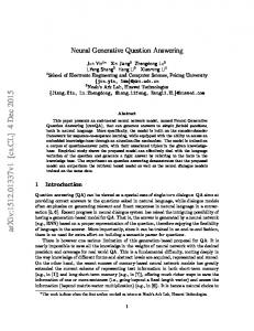
Figure 1. We encode the input scene as a graph representing objects and their spatial arrangement, and the input question as a graph representing words and their syntactic dependencies. A neural network is trained to reason over these representations, and produce a suitable answer as a prediction over an output vocabulary.

(they are usually referred to as “abstract scenes”, despite this being a misnomer). Our experiments focus on this dataset of clip art scenes, as they allow to focus on semantic reasoning and vision-language interactions, in isolation from the performance of visual recognition (see examples in Fig. 5.2). A particularly attractive version of this dataset was introduced in [31] by selecting only the questions with binary answers (e.g. yes/no) and pairing each image with a minimally-different complementary version that elicits the opposite (no/yes) answer (see examples in Fig. 5.2, bottom rows). This strongly contrasts with other VQA datasets of real images, where a correct answer is often obvious without looking at the image, by relying on systematic regularities of frequent questions and answers [4, 31]. The marginal improvements often reported on such datasets are difficult to interpret as actual progress in fine-grained scene understanding and reasoning, and this hampers the progress toward the greater goal of VQA. In our view, and despite obvious limitations of synthetic images, improvements on the aforementioned “balanced” dataset constitute a more robust sign of progress, since subtle details of the scenes must be considered to answer questions correctly.

1. Introduction The task of Visual Question Answering has received growing interest in the recent years [18, 4, 26]. It involves multiple aspects of computer vision, natural language processing, and artificial intelligence. In its common form, a question is provided as text in natural language together with an image, and a correct answer must be predicted, typically in the form of a single word or a short phrase. In a multiple-choice setting, candidate answers are provided, alleviating evaluation issues related to synonyms and paraphrasing. Multiple datasets for VQA have been introduced with either real [4, 15, 18, 22, 32] or synthetic images [4, 31]. Our experiments uses the latter, which contains clip art or “cartoon” images created by humans to depict realistic scenes

Challenges The questions in the clip-art dataset vary greatly in their complexity. Some can be directly answered from observations of visual elements, e.g. Is there a dog in 1

the room ?, or Is the weather good ? with the image of a sunny day. Others require relating multiple facts or understanding complex actions, e.g. Is the boy going to catch the ball?, or Is it the winter? about a scene containing a fireplace and jackets on a coat rack. A major challenge is the sparsity of training data. Even a large number of training questions (almost 25,000 for the clip art scenes of [4]) cannot possibly cover the combinatorial diversity of possible objects and concepts. Adding to this challenge, most methods for VQA process the question through a recurrent neural network (such as an LSTM) trained from scratch solely on the training questions.

and the question with an RNN (despite the fact that grammatical structure is very non-linear). The graph representation ignores the order in which elements are processed, but instead represents the relationships between different elements using different edge types. Our network uses multiple layers that iterate over the features associated with every node, then ultimately identifies a soft matching between nodes from the two graphs. This matching reflects the correspondences between the words in the question and the objects in the image. The features of the matched nodes then feed into a classifier to infer the answer to the question (Fig. 1).

Language representation The above reasons motivate us to take advantage of the extensive existing work in the natural language community to aid processing the questions. First, we identify the syntactic structure using a dependency parser [7]. This produces a graph representation of the question in which each node represents a word and each edge a particular type of dependency (e.g. determiner, nominal subject, direct object, etc.). Second, we associate each word (node) with a vector embedding pretrained on large corpora of text data [21]. This embedding maps the words to a space in which distances are semantically meaningful. Consequently, this essentially regularizes the remainder of the network to share learned concepts among related words and synonyms. This particularly helps dealing with rare words, and also allows questions to include words absent from the training questions/answers. Note that this pretraining and ad hoc processing of the language part mimics a practice common for the image part, in which visual features are usually obtained from a fixed CNN, itself pretrained on a larger dataset and with a different (supervised classification) objective.

The main contributions of this paper are four-fold. 1) We describe how to use graph representations of scene and question for VQA, and a neural network capable of processing these representations to infer an answer. 2) We show how the graph representation can take advantage of preprocessing the language part, using syntactic dependencies as edge features and word embeddings as nodes features. 3) We train the proposed model on the VQA “abstract scenes” benchmark [4] and demonstrate its efficacy by raising the state-of-the-art accuracy from 71.2% to 74.4% in the multiple-choice setting. On the “balanced” version of the dataset, we raise the accuracy from 34.7% to 39.1% in the hardest setting (requiring a correct answer over pairs of scenes). 4) We evaluate the uncertainty in the model by presenting – for the first time on the task of VQA – precision/recall curves of predicted answers. Those curves provide more insight than the single accuracy metric and favorably show that the uncertainty estimated by the model about its predictions correlates with the ambiguity of the human-provided ground truth.

Scene representation Each object in the scene corresponds to a node in the scene graph, which has an associated feature vector describing its appearance. The graph is fully connected, with each edge representing the relative position of the objects in the image. Applying Neural Networks to graphs The two graph representations feed into a deep neural network that we will describe in Section 4. The advantage of applying the Graph Neural Network (GNN) over text- and scene graphs, rather than on more typical representations is that the graphs can capture relationships between words and between objects. This enables the GNN to exploit (1) the unordered nature of some elements (the scene objects in particular) and (2) the semantic relationships between elements (grammatical relationships in particular). The unordered aspect contrasts with the typical approach of representing the image with CNN activations (which are sensitive to all object locations)

2. Related work The task of visual question answering has received increasing interest since the seminar paper of Antol et al. [4]. Most recent methods are based on the idea of a joint embedding of the image and the question using a deep neural network. The image is passed through a convolutional neural network (CNN) pretrained for image classification, from which intermediate features are extracted to describe the image. The question is typically passed through a recurrent neural network (RNN) such as an LSTM, which produces a fixed-size vector representing the sequence of words. These two representations are mapped to a joint space by one or several non-linear layers. They can then be fed into a classifier over an output vocabulary, predicting the final answer. Most recent papers on VQA propose improvements and variations on this basic idea. Consult [26] for a survey.

Input scene description and parsed question

Initial embedding

Graph processing

Combined features Objects

Ø

det Is

the

advmod

book

on

GRU Node Neighbours

fire ?

Weighted sum

Words

Affine projection

Word/vector embeddings

Prediction over candidate answers

Σ

Matching weights

Sigmoid or softmax

...

σ

yes 0.9 no 0.0

σ

Cosine similarity

nsubj cop

Figure 2. Architecture of the proposed neural network. The input is provided as a description of the scene (a list of objects with their visual characteristics) and a parsed question (words with their syntactic relations). The scene-graph contains a node with a feature vector for each object, and edge features that represent their spatial relationships. The question-graph reflects the parse tree of the question, with a word embedding for each node, and a vector embedding of types of syntactic dependencies for edges. A recurrent unit (GRU) is associated with each node of both graphs. Over multiple iterations, the GRU updates a representation of each node that integrates context from its neighbours within the graph. Features of all objects and all words are combined (concatenated) pairwise, and they are weighted with a form of attention. That effectively matches elements between the question and the scene. The weighted sum of features is passed through a final classifier that predicts scores over a fixed set of candidate answers.

A major improvement to the basic method is to use an attention mechanism [32, 28, 5, 13, 3, 29]. It models interactions between specific parts of the inputs (image and question) depending on their actual contents. The visual input is then typically represented a spatial feature map, instead of holistic, image-wide features. The feature map is used with the question to determine spatial weights that reflect the most relevant regions of the image. Our approach uses a similar weighting operation, which, with our graph representation, we equate to a subgraph matching. Graph nodes representing question words are associated with graph nodes representing scene objects and vice versa. Similarly, the co-attention model of Lu et al. [17] determines attention weights on both image regions and question words. Their best-performing approach proceeds in a sequential manner, starting with question-guided visual attention followed by image-guided question attention. In our case, we found that a joint, one-pass version performs better. A major contribution of our model is to use structured representations of the input scene and the question. This contrasts with typical CNN and RNN models which are limited to spatial feature maps and sequences of words respectively. The dynamic memory networks (DMN), applied to VQA in [27] also maintain a set-like representation of the input. As in our model, the DMN models interactions between different parts of the input. Our method can additionally take, as input, features characterizing arbitrary relations between parts of the input (the edge features in our graphs). This specifically allows making use of syntactic dependencies between words after pre-parsing the question. Most VQA systems are trained end-to-end from questions and images to answers, with the exception of the

visual feature extractor, which is typically a CNN pretrained for image classification. For the language processing part, some methods address the the semantic aspect with word embeddings pretrained on a language modeling task (e.g. [24, 10]). The syntactic aspect is often overlooked. In [31], hand-designed rules serve to identify primary and secondary objects of the questions. In the Neural Module Networks [3, 2], the question is processed by a dependency parser, and fragments of the parse, selected with ad hoc fixed rules are associated with modules, assembled into a full neural network. In contrast, our method is trained to make direct use of the output of a syntactic parser.

Several recent works have independently proposed similar formulations for processing graphs within neural networks [9, 12, 16]. Defferrard et al. [8] describes a comprehensive framework for applying convolutions and pooling over graphs. Most similar to ours are the Gated Graph Sequence Neural Networks [16], which associate a gated recurrent unit (GRU [6]) to each node, and update the feature vector of each node by iteratively passing messages between neighbours. Also related is the work of Vinyals et al. for embedding a set into fixed-size vector [25]. They feed the entire set through a recurrent unit multiple times, so that the final state incorporates information from all elements of the set, while being invariant to the order in which they are represented. Each recurrent iteration uses an attention mechanism to focus on different parts of the input set. Our formulation similarly incorporates information from neighbours into each node feature over multiple iterations, but we did not find any advantage in using an attention mechanism within the recurrent unit.

3. Graph representation of scenes and questions The input data for each training or test instance is a text question and the description of a scene. The question is processed with the Stanford dependency parser [7], which outputs the following. •

•

A set of N Q words that constitute the nodes of the question graph. Each word is represented by its index in the Q input vocabulary, a token xQ i ∈ Z (i ∈ 1..N ). A set of pairwise relations between words, which constitute the edges of our graph. An edge between words i and j is represented by eQ ij ∈ Z, an index among the possible types of dependencies.

The scene is represented as follows. •

•

A set of N S objects that constitute the nodes of the scene graph. Each node is represented by a vector xSi ∈ RC of visual features (i ∈ 1..N S ). A set of pairwise relations between all objects. They form the edges of a fully-connected graph of the scene. The edge between objects i and j is represented by a vector eSij ∈ RD that encodes relative spatial relationships.

Our experiments are carried out on datasets of clip art scenes, in which descriptions of the scenes are provided in the form of lists of objects with their visual features. The method is equally applicable to real images, with the object list replaced by candidate object detections. Our experiments on clip art allows the effect of the proposed method to be isolated from the performance of the object detector. Please refer to the supplementary material for implementation details. The features of all nodes and edges are projected to a vector space RH of common dimension (typically H=300). The question nodes and edges use vector embeddings implemented as look-up tables, and the scene nodes and edges use affine projections:   0 xiQ = W1 xQ i 0

xiS

=

W3 xSi

+ b3

  0 eijQ = W2 eQ ij 0

eijS

=

W4 eSij

+ b4

(1) (2)

with W1 the word embedding (usually pretrained, see supplementary material), W2 the embedding of dependencies, W3 ∈ Rh×c and W4 ∈ Rh×d weight matrices, and b3 ∈ Rc and b4 ∈ Rd biases.

4. Processing graphs with neural networks We now describe a deep neural network suitable for processing the question and scene graphs to infer an answer. See Fig. 2 for an overview. The two graphs representing the question and the scene are processed independently in a recurrent architecture. We

drop the exponents S and Q for this paragraph as the same procedure applies to both graphs. Each node xi is associated with a gated recurrent unit (GRU [6]) and processed over a fixed number T of iterations (typically T =4): h0i = 0 hti

=

ni =

GRU ht−1 , [x0i i pool( e0ij ◦ x0j ) j

(3) ; ni ]




t ∈ [1, T ]

(4) (5)

Square brackets with a semicolon represent a concatenation of vectors and ◦ the Hadamard (element-wise) product. The final state of the GRU is used as the new representation of the nodes: x00i = hTi . The pool operation transforms features from a variable number of neighbours (i.e. connected nodes) to a fixed-size representation. Any commutative operation can be used (e.g. sum, maximum). In our implementation, we found the best performance with the average function, taking care of averaging over the variable number of connected neighbours. An intuitive interpretation of the recurrent processing is to progressively integrate context information from connected neighbours into each node’s own representation. Our formulation is similar but slightly different from the gated graph networks [16], as the propagation of information in our model is limited to the first order. Note that our graphs are typically densely connected. We now introduce a form of attention into the model, which constitutes an essential part of the model. The motivation is two-fold: (1) to identify parts of the input data most relevant to produce the answer and (2) to align the elements of the question with those of the scene. Practically, we estimate the relevance of each possible pairwise combinations of words and objects. More precisely, we compute scalar “matching weights” between node sets S {xQ i } and {xi }. These weights are comparable to the “attention weights” in other models (e.g. [17]). Therefore, ∀ i ∈ 1..N Q , j ∈ 1..N S : ! 0  x0 Q xjS  i ◦ 0 + b5 (6) aij = σ W5 0 kxiQ k kxjS k where W5 ∈ R1×h and b5 ∈ R are learned weights and biases, and σ the logistic function that introduces a nonlinearity and bounds the weights to ]0, 1[. The formulation is similar to a cosine similarity with learned weights on the feature dimensions. Note that the weights are computed using the initial embedding of the node features (pre-GRU). We apply the scalar weights aij to the corresponding pairwise combinations of question and scene features, thereby focusing and giving more importance to the matched pairs (Eq. 7). We sum the weighted features over the scene elements (Eq. 8) then over the question elements (Eq. 9), interleaving the sums with affine projections

and non-linearities to obtain a final prediction: S yij = aij ◦ [xQ i ; xj ]
PN S yi0 = f W6 j yij + b6
PN Q y 00 = f 0 W7 i yi0 + b7

(7) (8) (9)

with W6 , W7 , b6 , b7 learned weights and biases, f a ReLU, and f 0 a softmax or a logistic function (see experiments, Section 5.1). The summations over the scene elements and question elements is a form of pooling that brings the variable number of features (due to the variable number of words and objects in the input) to a fixed-size output. The final output vector y 00 ∈ RT contains scores for the possible answers, and has a number of dimensions equal to 2 for the binary questions of the “balanced” dataset, or to the number of all candidate answers in the “abstract scenes” dataset. The candidate answers are those appearing at least 5 times in the training set (see supplementary material for details).

5. Evaluation Datasets Our evaluation use two datasets: the original “abstract scenes” from Antol et al. [4] and its “balanced” extension [31]. They both contain scenes created by humans in a drag-and-drop interface for arranging clip art objects and figures. The original dataset contains 20k/10k/20k scenes (for training/validation/test respectively) and 60k/30k/60k questions, each with 10 humanprovided ground-truth answers. Questions are categorized based on the type of the correct answer into yes/no, number, and other, but the same method is used for all categories, the type of the test questions being unknown. The “balanced” version of the dataset contains only the subset questions which have binary (yes/no) answers and, in addition, complementary scenes created to elicit the opposite answer to each question. This is significant because guessing the modal answer from the training set will the succeed only half of the time (slightly more than 50% in practice because of disagreement between annotators) and give 0% accuracy over complementary pairs. This contrasts with other VQA datasets where blind guessing can be very effective. The pairs of complementary scenes also typically differ by only one or two objects being displaced, removed, or slightly modified (see examples in Fig. 5.2, bottom rows). This makes the questions very challenging by requiring to take into account subtle details of the scenes. Metrics The main metric is the average “VQA score” [4], which is a soft accuracy that takes into account variability of ground truth answers from multiple human annotators. Let us refer to a test question by an index q = 1..M , and to each possible answer in the output vocabulary by an index a. The

ground truth score s(q, a) = 1.0 if the answer a was provided by m≥3 annotators. Otherwise, s(q, a) = m/31 . Our method outputs a predicted score sˆ(q, a) for each question and answer (y 00 in Eq. 9) and the overall accuracy is the average groundPtruth score of the highest prediction per quesM 1 ˆ(q, a)). tion, i.e. M q s(q, arg maxa s It has been argued that the “balanced” dataset can better evaluate a method’s level of visual understanding than other datasets, because it is less susceptible to the use of language priors and dataset regularities (i.e. guessing from the question[31]). Our initial experiments confirmed that the performances of various algorithms on the balanced dataset were indeed better separated, and we used it for our ablative analysis. We also focus on the hardest evaluation setting [31], which measures the accuracy over pairs of complementary scenes. This is the only metric in which blind models (guessing from the question) obtain null accuracy. This setting also does not consider pairs of test scenes deemed ambiguous because of disagreement between annotators. Each test scene is still evaluated independently however, so the model is unable to increase performance by forcing opposite answers to pairs of questions. The metric is then a standard “hard” accuracy, i.e. all ground truth scores s(i, j) ∈ {0, 1}. Please refer to the supplementary material for additional details.

5.1. Evaluation on the “balanced” dataset We compare our method against the three models proposed in [31]. They all use an ensemble of models exploiting either an LSTM for processing the question, or an elaborate set of hand-designed rules to identify two objects as the focus of the question. The visual features in the three models are respectively empty (blind model), global (scenewide), or focused on the two objects identified from the question. These models are specifically designed for binary questions, whereas ours is generally applicable. Nevertheless, we obtain significantly better accuracy than all of the three (Table 1). Differences in performance are mostly visible in the “pairs” setting, which we believe is more reliable as it discards ambiguous test questions on which human annotators disagreed. During training, we take care of keeping pairs of complementary scenes together when forming mini-batches. This has a significant positive effect on the stability of the optimization. Interestingly, we did not notice any tendency toward overfitting when training on balanced scenes. We hypothesize that the pairs of complementary scenes have a strong regularizing effect that force the learned model to focus on relevant details of the scenes. In Fig. 5.2 (and in the supplementary material), we visualize the matching weights between question words and scene objects (Eq. 6). As expected, these tend to be larger between semantically related 1 Ground

truth scores are also averaged in a 10–choose–9 manner [4].

1

0.8

0.8

0.8

0.6 Softmax, soft scores AP=76.3% F1=71.2%

0.4

Sigmoid, soft scores AP=72.9% F1=69.0%

0.2

0.6 Softmax, soft scores AP=67.1% F1=64.9%

0.4

Sigmoid, soft scores AP=67.0% F1=65.3%

0.2

Softmax, hard scores AP=72.3% F1=68.2%

Precision

1

Precision

Precision

1

0.6

0

0.2

0.4

0.6

0.8

1

Sigmoid, soft scores AP=78.7% F1=76.6%

0.2

Softmax, hard scores AP=63.1% F1=62.8%

0

0

Softmax, soft scores AP=78.1% F1=76.9%

0.4

Softmax, hard scores AP=78.7% F1=76.7%

0 0

0.2

Recall

0.4

0.6

0.8

1

0

0.2

Recall

0.4

0.6

0.8

1

Recall

Figure 3. Precision/recall on the “abstract scenes” (left: multiple choice, middle: open-ended) and “balanced” datasets (right). The scores assigned by the model to predicted answers is a reliable measure of its certainty: a strict threshold (low recall) filters out incorrect answers and produces a very high precision. On the “abstract scenes” dataset (left and middle), a slight advantage is brought by training for soft target scores that capture ambiguities in the human-provided ground truth.

elements (e.g. daytime↔sun, dog↔puppy, boy↔human) although some are more difficult to interpret. Our best performance of about 39% is still low in absolute terms, which is understandable from the wide range of concepts involved in the questions (see examples in Fig. 5.2 and in the supplementary material). It seems unlikely that these concepts could be learned from training question/answers alone, and we suggest that any further significant improvement in performance will require external sources of information at training and/or test time.

Avg. score Avg. accuracy Method

over scenes

Zhang et al. [31] blind

63.33

0.00

with global image features

71.03

23.13

with attention-based image features

74.65

34.73

74.94

39.1

Graph VQA (full model) (1)

Question: no parsing (graph with previous/next edges) 37.9

(2)

Question: word embedding not pretrained

33.8

0

(eijS =1)

(3)

Scene: no edge features

(4)

Graph processing: disabled for question (xi Q =xiS )

36.8 00

00

Ablative evaluation We evaluated variants of our model to measure the impact of various design choices (see numbered rows in Table 1). On the question side, we evaluate (row 1) our graph approach without syntactic parsing, building question graphs with only two types of edges, previous/next and linking consecutive nodes. This shows the advantage of using the graph method together with syntactic parsing. Optimizing the word embeddings from scratch (row 2) rather than from pretrained Glove vectors [21] produces a significant drop in performance. On the scene side, we removed the edge features (row 3) by setting eSij = 1. It confirms that the model makes use of the spatial relations between objects encoded by the edges of the graph. In rows 4–6, we disabled the recurrent graph processing (x00i = x0i ) for the either the question, the scene, or both. Although the performance is affected in all cases, it is most significant for the question. The language part thus benefits the most from the graph processing. We finally tested the model with uniform matching weights (aij = 1, row 10). As expected, it performed poorly. Our weights act similarly to the attention mechanisms in other models (e.g. [32, 28, 5, 13, 29]) and our observations confirm that such mechanisms are crucial for good performance.

over pairs

S

0

0

Q

37.1

(5)

Graph processing: disabled for scene (xi =xi )

37.0

(6)

Graph processing: disabled for question/scene

35.7

(7)

Graph processing: only 1 iteration for question (T Q =1) 39.0

(8)

Graph processing: only 1 iteration for scene (T S =1)

37.9

(9)

Graph processing: only 1 iteration for question/scene

39.1

(10)

No matching weights (aij =1)

24.4

Table 1. Results on the test set of the “balanced” dataset [31] (in percents , using balanced versions of both training and test sets). Numbered rows report accuracy over pairs of complementary scenes for ablated versions of our method.

Precision/recall We are interested in assessing the confidence of our model in its predicted answers. Most existing VQA methods treat the answering as a hard classification over candidate answers, and almost all reported results consist of a single accuracy metric. To provide more insight, we produce precision/recall curves for predicted answers. A precision/recall point (p, r) is obtained by setting a thresh-

Acuracy over pairs of scenes

0.4

0.3

0.2

Full model Without syntactic parsing Without pretrained word embedding Without pretrained word embedding/syntactic parsing

0.1

0 0.1

0.2

0.3

0.4

0.5

0.6

0.7

0.8

0.9

1

Fraction of training set used

Figure 4. Impact of the amount of training data on performance (accuracy over pairs on the “balanced” dataset). Language preprocessing always improve generalization: pre-parsing and pretrained word embeddings both have a positive impact individually, and their effects are complementary to each other.

old t on predicted scores such that
P ˆ(i, j)>t s(i, j) i,j 1 s P p= s(i, j)>t) i,j 1(ˆ
P ˆ(i, j)>t s(i, j) i,j 1 s P r= i,j s(i, j)

(10)

larly, paraphrases of similar questions should produce parse graphs with more similarities than a simple concatenation of words would reveal (as in the input to traditional LSTMs). We trained our model with limited subsets of the training data (see Fig. 5.1). Unsurprisingly, the performance grows steadily with the amount of training data, which suggests that larger datasets would improve performance. In our opinion however, it seems unlikely that sufficient data, covering all possible concepts, could be be collected in the form of question/answer examples. More data can however be brought in with other sources of information and supervision. Our use of parsing and word embeddings is a small step in that direction. Both techniques clearly improve generalization (Fig. 5.1). The effect may be particularly visible in our case because of the relatively small number of training examples (about 20k questions in the “balanced” dataset). It is unclear whether huge VQA datasets could ultimately negate this advantage. Future experiments on larger datasets (e.g. [15]) may answer this question.

5.2. Evaluation on the “abstract scenes” dataset (11)

where 1(·) is the 0/1 indicator function. We plot precision/recall curves in Fig. 5 for both datasets2 . The predicted score proves to be a reliable indicator of the model confidence, as a low threshold can achieve near-perfect accuracy (Fig. 5, left and middle) by filtering out harder and/or ambiguous test cases. We compare models trained with either a softmax or a sigmoid as the final non-linearity (Eq. 9). The common practice is to train the softmax for a hard classification objective, using a cross-entropy loss and the answer of highest ground truth score as the target. In an attempt to make better use of the multiple human-provided answers, we propose to use the soft ground truth scores as the target with a logarithmic loss. This shows an advantage on the “abstract scenes” dataset (Fig. 5, left and middle). In that dataset, the soft target scores reflect frequent ambiguities in the questions and the scenes, and when synonyms constitute multiple acceptable answers. In those cases, we can avoid the potential confusion induced by a hard classification for one specific answer. The “balanced” dataset, by nature, contains almost no such ambiguities, and there is no significant difference between the different training objectives (Fig. 5, right). Effect of training set size Our motivation for introducing language parsing and pretrained word embeddings is to better generalize the concepts learned from the limited training examples. Words representing semantically close concepts ideally get assigned close word embeddings. Simi2 The “abstract scenes” test set is not available publicly, and precision/recall can only be provided on its validation set.

We report our results on the original “abstract scenes” dataset in Table 2. The evaluation is performed on an automated server that does not allow for an extensive ablative analysis. Anecdotally, performance on the validation set corroborates all findings presented above, in particular the strong benefit of pre-parsing, pretrained word embeddings, and graph processing with a GRU. At the time of our submission, our method occupies the top place on the leader board in both the open-ended and multiple choice settings. The advantage over existing method is most pronounced on the binary and the counting questions. Refer to Fig. 5.2 and to the supplementary for visualizations of the results.

6. Conclusions We presented a deep neural network for visual question answering that processes graph-structured representations of scenes and questions. This enables leveraging existing natural language processing tools, in particular pretrained word embeddings and syntactic parsing. The latter showed significant advantage over a traditional sequential processing of the questions, e.g. with LSTMs. In our opinion, VQA systems are unlikely to learn everything from question/answer examples alone. We believe that future leaps in performance will require additional sources of information and supervision. Our explicit processing of the language part is a small step in that direction. It was clearly shown to improve generalization without resting entirely on VQAspecific annotations. We have so far applied our method to datasets of clip art scenes. Its direct extension to real images will be addressed in future work, by replacing nodes in the input scene graph with proposals from pretrained object detectors.

Method

Multiple choice Yes/no Other

Overall

Number

Overall

Open-ended Yes/no Other

Number

LSTM blind [4] LSTM with global image features [4] Zhang et al. [31] (yes/no only) Multimodal residual learning [14] U. Tokyo MIL (ensemble) [23, 1]

61.41 69.21 35.25 67.99 71.18

76.90 77.46 79.14 79.08 79.59

49.19 66.65 — 61.99 67.93

49.65 52.90 — 52.57 56.19

57.19 65.02 35.25 62.56 69.73

76.88 77.45 79.14 79.10 80.70

38.79 56.41 — 48.90 62.08

49.55 52.54 — 51.60 58.82

Graph VQA (full model)

74.37

79.74

68.31

74.97

70.42

81.26

56.28

76.47

Table 2. Results on the test set of the “abstract scenes” dataset (average scores in percents).

plant

picture

window

rug

window

rug

desk

picture moon

sofa

picture cloud

cat

human

human

What is the boy holding ? Answer: toy blocks

window

plant

picture

picture

dog

human

Is the dog sleeping or resting ? Answer: sleeping

is what the is dog the sleeping boy or holding resting

is

is

the

the

dog

dog

white

white

is

couch

puppy

scooter

duck

duck

cloud

human

Is it daytime ? Answer: no

sun

scooter

duck

duck

human

Is it daytime ? Answer: yes

human

rug

human

Is the dog white ? Answer: no

picture

picture

couch

puppy

human

human

Is the dog white ? Answer: yes

is

it

it

daytime

daytime

Figure 5. Qualitative results on the “abstract scenes” dataset (top row) and on “balanced” pairs (middle and bottom row). We show the input scene, the question, the predicted answer, and the correct answer when the prediction is erroneous. We also visualize the matrices of matching weights (Eq. 6, brighter correspond to higher values) between question words (vertically) and scene objects (horizontally). The matching weights are also visualized over objects in the scene, after summation over words, giving an indication of their estimated relevance. The ground truth object labels are for reference only, and not used for training nor inference.

References [1] VQA Challenge leaderboard. http://visualqa.org/ challenge.html. 8 [2] J. Andreas, M. Rohrbach, T. Darrell, and D. Klein. Learning to compose neural networks for question answering. In Annual Conference of the North American Chapter of the Association for Computational Linguistics, 2016. 3 [3] J. Andreas, M. Rohrbach, T. Darrell, and D. Klein. Neural Module Networks. In Proc. IEEE Conf. Comp. Vis. Patt. Recogn., 2016. 3 [4] S. Antol, A. Agrawal, J. Lu, M. Mitchell, D. Batra, C. L. Zitnick, and D. Parikh. VQA: Visual Question Answering. In Proc. IEEE Int. Conf. Comp. Vis., 2015. 1, 2, 5, 8 [5] K. Chen, J. Wang, L.-C. Chen, H. Gao, W. Xu, and R. Nevatia. ABC-CNN: An Attention Based Convolutional Neural Network for Visual Question Answering. arXiv preprint arXiv:1511.05960, 2015. 3, 6 [6] K. Cho, B. van Merrienboer, C. Gulcehre, F. Bougares, H. Schwenk, and Y. Bengio. Learning phrase representations using RNN encoder-decoder for statistical machine translation. In Proc. Conf. Empirical Methods in Natural Language Processing, 2014. 3, 4 [7] M.-C. de Marneffe and C. D. Manning. The stanford typed dependencies representation. In COLING Workshop on Cross-framework and Cross-domain Parser Evaluation, 2008. 2, 4, 10 [8] M. Defferrard, X. Bresson, and P. Vandergheynst. Convolutional neural networks on graphs with fast localized spectral filtering. In Proc. Advances in Neural Inf. Process. Syst., 2016. 3 [9] D. K. Duvenaud, D. Maclaurin, J. Aguilera-Iparraguirre, R. G´omez-Bombarelli, T. Hirzel, A. Aspuru-Guzik, and R. P. Adams. Convolutional networks on graphs for learning molecular fingerprints. arXiv preprint arXiv:1509.09292, 2015. 3 [10] A. Fukui, D. H. Park, D. Yang, A. Rohrbach, T. Darrell, and M. Rohrbach. Multimodal compact bilinear pooling for visual question answering and visual grounding. arXiv preprint arXiv:1606.01847, 2016. 3 [11] X. Glorot and Y. Bengio. Understanding the difficulty of training deep feedforward neural networks. In Proc. Int. Conf. Artificial Intell. & Stat., pages 249–256, 2010. 10 [12] A. Jain, A. R. Zamir, S. Savarese, and A. Saxena. Structuralrnn: Deep learning on spatio-temporal graphs. In Proc. IEEE Conf. Comp. Vis. Patt. Recogn., 2016. 3 [13] A. Jiang, F. Wang, F. Porikli, and Y. Li. Compositional Memory for Visual Question Answering. arXiv preprint arXiv:1511.05676, 2015. 3, 6 [14] J.-H. Kim, S.-W. Lee, D.-H. Kwak, M.-O. Heo, J. Kim, J.W. Ha, and B.-T. Zhang. Multimodal residual learning for visual qa. arXiv preprint arXiv:1606.01455, 2016. 8 [15] R. Krishna, Y. Zhu, O. Groth, J. Johnson, K. Hata, J. Kravitz, S. Chen, Y. Kalantidis, L.-J. Li, D. A. Shamma, M. Bernstein, and L. Fei-Fei. Visual genome: Connecting language and vision using crowdsourced dense image annotations. arXiv preprint arXiv:1602.07332, 2016. 1, 7

[16] Y. Li, D. Tarlow, M. Brockschmidt, and R. S. Zemel. Gated graph sequence neural networks. arXiv preprint arXiv:1511.05493, 2015. 3, 4 [17] J. Lu, J. Yang, D. Batra, and D. Parikh. Hierarchical question-image co-attention for visual question answering. arXiv preprint arXiv:1606.00061, 2016. 3, 4 [18] M. Malinowski and M. Fritz. A multi-world approach to question answering about real-world scenes based on uncertain input. In Proc. Advances in Neural Inf. Process. Syst., pages 1682–1690, 2014. 1 [19] J. Pennington, R. Socher, and C. Manning. Glove: Global vectors for word representation. http://nlp. stanford.edu/projects/glove/. 10 [20] J. Pennington, R. Socher, and C. Manning. Stanford dependency parser website. http://nlp.stanford.edu/ software/stanford-dependencies.shtml. 10 [21] J. Pennington, R. Socher, and C. Manning. Glove: Global Vectors for Word Representation. In Conference on Empirical Methods in Natural Language Processing, 2014. 2, 6, 10 [22] M. Ren, R. Kiros, and R. Zemel. Image Question Answering: A Visual Semantic Embedding Model and a New Dataset. In Proc. Advances in Neural Inf. Process. Syst., 2015. 1 [23] K. Saito, A. Shin, Y. Ushiku, and T. Harada. Dualnet: Domain-invariant network for visual question answering. arXiv preprint arXiv:1606.06108, 2016. 8 [24] K. J. Shih, S. Singh, and D. Hoiem. Where to look: Focus regions for visual question answering. In Proc. IEEE Conf. Comp. Vis. Patt. Recogn., 2016. 3 [25] O. Vinyals, S. Bengio, and M. Kudlur. Order matters: Sequence to sequence for sets. arXiv preprint arXiv:1511.06391, 2015. 3 [26] Q. Wu, D. Teney, P. Wang, C. Shen, A. Dick, and A. van den Hengel. Visual Question Answering: A Survey of Methods and Datasets. arXiv preprint arXiv:1607.05910, 2016. 1, 2 [27] C. Xiong, S. Merity, and R. Socher. Dynamic memory networks for visual and textual question answering. In Proc. Int. Conf. Mach. Learn., 2016. 3 [28] H. Xu and K. Saenko. Ask, Attend and Answer: Exploring Question-Guided Spatial Attention for Visual Question Answering. arXiv preprint arXiv:1511.05234, 2015. 3, 6 [29] Z. Yang, X. He, J. Gao, L. Deng, and A. Smola. Stacked Attention Networks for Image Question Answering. In Proc. IEEE Conf. Comp. Vis. Patt. Recogn., 2016. 3, 6 [30] M. D. Zeiler. ADADELTA: an adaptive learning rate method. arXiv preprint arXiv:1212.5701, 2012. 10 [31] P. Zhang, Y. Goyal, D. Summers-Stay, D. Batra, and D. Parikh. Yin and yang: Balancing and answering binary visual questions. In Proc. IEEE Conf. Comp. Vis. Patt. Recogn., 2016. 1, 3, 5, 6, 8 [32] Y. Zhu, O. Groth, M. Bernstein, and L. Fei-Fei. Visual7W: Grounded Question Answering in Images. In Proc. IEEE Conf. Comp. Vis. Patt. Recogn., 2016. 1, 3, 6

Supplementary material A. Implementation details We provide below practical details of our implementation of the proposed method. •

•

•

•

•

•

•

•

Size of vector embeddings of node features, edge features, and all hidden states within the network: H=300. Note that smaller values such as H=200 also give very good results (not reported in this paper) at a fraction of the training time. Number of recurrent iterations to update graph node representations: T Q =T S =4. Anecdotally, we observed that processing the scene graph benefits from more iterations than the question graph, for which performance nearly saturates with 2 or more iterations. As reported in the ablative evaluation (Table 1), the use of at least a single iteration has a stronger influence than its exact number. All weights except word embeddings are initialized randomly following [11]. Word embeddings are initialized with Glove vectors [21] of dimension 300 available publicly [19], trained for 6 billion words on Wikipedia and Gigaword. The word embeddings are fine-tuned with a learning rate of 1/10 of the other weights. Dropout with ratio 0.3 is applied between the weighted sum over scene elements (Eq. 8) and the final classifier (Eq. 9). Weights are optimized with Adadelta [30] with minibatches of 128 questions. We run optimization until convergence (typically 20 epochs on the “abstract scenes”, 100 epochs on the “balanced” dataset) and report performance on the test set from the epoch with the highest performance on the validation set (measured by VQA score on the “abstract scenes” dataset, and accuracy over pairs on the “balanced” dataset). The edges between word nodes in the input question graph are labeled with the dependency labels identified by the Stanford parser [7, 20]. These dependencies are directed, and we supplement all of them with their symmetric, albeit tagged with a different set of labels. The output of the parser includes the propagation of conjunct dependencies (its default setting). This yields quite densely connected graphs. The input features of the object nodes are those directly available in the datasets. They represent: the object category (human, animal, small or large object) as one onehot vector, the object type (table, sun, dog window, ...) as a one-hot vector, the expression/pose/type (various depictions being possible for each object type) as a one-hot vector, and 10 scalar values describing the pose of human figures (the X/Y position of arms, legs, and head relative

•

•

•

•

to the torso). They form altogether a feature vector of dimension 159. The edge features between objects represent: the signed difference in their X/Y position, the inverse of their absolute difference in X/Y position, and their relative position on depth planes as +1 if closer (potentially occluding the other), -1 otherwise. All input features are normalized for zero mean and unit variance. When training for the “balanced” dataset, care is taken to keep each pair of complementary scenes in a same minibatch when shuffling training instances. This has a noticeable effect on the stability of the optimization. In the open-ended setting, the output space is made of all answers that appear at least 5 times in the training set. These correspond to 623 possible answers, which cover 96% of the training questions. Our model was implemented in Matlab from scratch. Training takes in the order of 5 to 10 hours on one CPU, depending on the dataset and on the size H of the internal representations.

B. Additional results We provide below additional example results in the same format as in Fig. 5.2.

B.1. Additional results: abstract scenes dataset

is

jumprope

monkeybars

sun

cloud

bee

human

human

pillow

What is the girl doing ? Answer: jumping jumping rope

rug

door

desk

couch

plant

coatrack

human

human

Is the woman exercising ? Answer: yes

what is

the the woman girl

exercising

doing

endtable

fireplace

door

tv

chair

window

human

puppy

Is the man sitting on the armrest ? Answer: no yes

jumprope

soccer

football

sidewalk

pond

tree

bench

bush

human

Does he walk like an idiot ? Answer: yes

is does the he man walk sitting like on an the idiot armrest

what

who

color

is

are

sitting

the

between

pillows

toys

on the couch

notebook

rug

picture

window

couch

kitten

What color are the pillows on the couch ? Answer: brown human

doll

doll

couch

rug

window

window

human

Who is sitting between toys ? Answer: baby

might

shovel

sandbox

bench

tree

tree

slide

bird

butterfly

human

human

marshmallow

basket

ribs

Where is the girl sitting ? Answer: sandbox bench

bottle

apple

blanket

tree

grill

human

human

Might they be dating ? Answer: yes

where is

they

the

be

girl

dating

sitting

hotdog

sandbox

bench

slide

sidewalk

puppy

human

human

human

Where is the slide facing ? Answer: sandbox left

picture

window

window

rug

plant

fireplace

human

What is underneath the arched window ? Answer: rug plant

where

what

is

is

the

underneath the

slide

arched

facing

window

book

book

stool

stool

book

notebook

bookshelf

fireplace

sofa

window

bush

bush

blanket

bluejay

butterfly

butterfly

human

human

human

human

human

Is the lady reading ? Answer: yes

How many clouds ? Answer: 2

is

how

the

many

lady

clouds

reading

what

flowers

is

are

on

in

the

the

mantle

room

picture

diningtable

fireplace

window

dog

dog

human

how many

cat

What is on the mantle ? Answer: wine toys

petbed

couch

rug

desk

chair

plant

cat

human

How many flowers are in the room ? Answer: 0

this

pillow

picture

sofa

rug

puppy

human

can

fireplace

Does the man look depressed ? Answer: yes

dollhouse

toy

sofa

picture

picture

rug

human

Can this child climb on the couch ? no

does

child

the

climb

man

on

look

the

depressed

couch

sun

tree

bush

cloud

cloud

cloud

dog

human

How many clouds in the sky ? Answer: 3

lilypad

pond

cloud

tree

dog

human

What color is his shirt ? Answer: red black

how what many color clouds is in his the shirt sky

fireplace soccer

is

is

the

the

pattern

man

on

doing

the curtains

is

an

the

african

grass

american

green

girl

tree

cloud

cloud

human

is this

puppy

Is the grass green ? Answer: yes

rug

plant

coffeetable

picture

couch

window

window

cat

kitten

human

Is this an african american girl ? Answer: yes no

window

picture sun

what

what

window

sofa sandbox

sofa

mouse

kitten

human

human

What is the pattern on the curtains ? floral

table

coatrack

chair

tv

puppy

human

What is the man doing ? Answer: sitting watching tv

B.2. Additional results: balanced dataset

is

is

the

the

young

young

lady

lady

tempted

tempted

to

to

pet

pet

the

the

dog

dog

is

is

she

she

running

running

to

to

help

help

him

him

is the

man

man

close

close

to

to

the

the

left

left

window

window

door

picture

picture

rug couch

rug

window

window

picture

window

window

coatrack

picture

picture

human

is the

rug

Is the man close to the left window ? Answer: no yes

window

window

coatrack

picture

picture

rug

human

Is the man close to the left window ? Answer: yes no

human

human

Is she running to help him ? Answer: yes no

couch

rug

window

window

picture

human

human

Is she running to help him ? Answer: yes

puppy

human

Is the young lady tempted to pet the dog ? Answer: no

rug

door

picture

picture

puppy

human

Is the young lady tempted to pet the dog ? Answer: yes

is

is

the

the

dog

dog

white

white

is

is

this

this

picture

picture

couch

puppy

rug

doll

popcan

sandwich

sandwich

petbed

bookshelf

door

diningtable

couch

human

doll

popcan

sandwich

Is this man hungry ? Answer: yes no sandwich

petbed

bookshelf

door

diningtable

couch

human

Is this man hungry ? Answer: no yes

human

rug

human

Is the dog white ? Answer: no

picture

picture

couch

puppy

human

human

Is the dog white ? Answer: yes

is

is

the

the

girl

girl

about

about

to

to

kick

kick

the

the

soccer

soccer

ball

ball

is there

a

a

dog

dog

in

in

the

the

dog

dog

bed

bed

football

slide

sun

monkeybars

petbed

window

window

plant

puppy

is there

couch

Is there a dog in the dog bed ? Answer: no

petbed

window

window

plant

couch

puppy

Is there a dog in the dog bed ? Answer: no yes

human

human

soccer

slide

sun

Is the girl about to kick the soccer ball ? Answer: no

monkeybars

Is the girl about to kick the soccer ball ? Answer: no yes human

man hungry

human

man hungry

is the

young

young

man

man

dropping

dropping

a

a

football

football

is

is

there

there

a

a

dog

dog

is the

man

man

jump

jump

roping

roping

mushroom

mushroom

tree

football

bird

bush

tree

bush

bush

butterfly

butterfly

butterfly

pond

koi

duck

sidewalk

tree

cloud

cloud

human

is the

human

Is the man jump roping ? Answer: no

jumprope

sidewalk

tree

cloud

cloud

human

human

Is the man jump roping ? Answer: no yes

duck

chipmunk

bush

bush

bush

sun

pond

Is there a dog ? Answer: no

koi

duck

duck

dog

chipmunk

Is there a dog ? Answer: yes

bush

out

bird

sun

out

bush

sun

bird

is the

sun

is the

butterfly

pigeon

bush

sun

bird

bird

bird

Is the sun out ? Answer: no

butterfly

butterfly

butterfly

butterfly

pigeon

Is the sun out ? Answer: yes

sun

human

is the

cloud

Is the young man dropping a football ? Answer: yes no

mushroom

mushroom

football

tree

sun

cloud

human

Is the young man dropping a football ? Answer: yes