Greedy Geographic Routing is Good Enough in. Sensing Covered Networks. Guoliang Xing, Chenyang Lu, Robert Pless, Qingfeng Huang. {xing,lu,pless ...
1
Greedy Geographic Routing is Good Enough in Sensing Covered Networks Guoliang Xing, Chenyang Lu, Robert Pless, Qingfeng Huang {xing,lu,pless,qingfeng}@cse.wustl.edu Department of Computer Science and Engineering Washington University St. Louis, MO 63130, USA.
Abstract— This paper presents a theoretical analysis of greedy geographic routing protocols on a common class of wireless sensor networks that must provide sensing coverage over a geographic area. Contrary to well known results on random networks, we prove that the Greedy Geographic Forwarding and our new greedy protocol always succeed in any sensing covered network when the communication range is at least twice the sensing range. Furthermore, we derive the analytic upper bound for the network dilation of sensing covered networks and quantify its relationship with the ratio between communication range and sensing range. Simulations show that, when the ratio between communication range and sensing range reaches 4.5, the studied greedy routing protocols can find network paths whose hop count on a sensing covered network approaches 1.5 times that of an ideal network. These results provide several important insights into the design of sensor networks. Simple greedy geographic routing protocols are “good enough” in this class of wireless sensor networks, and more sophisticated routing protocols designed to handle routing voids are not necessary. In addition, redundant sensors can be turned off without significant loss in communication performance as long as the remaining active nodes maintain sensing coverage. This result provides a theoretical justification of sensing coverage control protocols that conserve energy through sleep schedules. Index Terms— Graph theory, System design, Ad hoc & sensor networks
I. I NTRODUCTION Wireless sensor networks represent a new type of ad hoc networks targeted at large scale distributed microsensing applications. Each node in such a network is a tiny device that integrates MEMS sensors, wireless interface, and processing units in a single hardware platform. While sensor networks share many similarities with traditional ad hoc networks comprised of laptops, they also face new requirements due to the sensing nature of their applications. In particular, many critical applications (e.g., distributed detection [1], distributed tracking and classifica-
tion [2]) introduce fundamental requirement of sensing coverage that does not exist in traditional ad hoc networks. In a sensing covered network, every point in a geographic area of interest must be within the sensing range of a specific number (one or more) of sensors. The problem of providing sensing coverage has received significant attention. Several algorithms and deployment strategies [3][4][5][6] were presented to achieve sensing coverage when a sensor network is deployed. Other projects [7][8][9] developed online energy conservation protocols that dynamically maintain sensing coverage using a subset of nodes while turning off redundant nodes. Complimentary to existing work that focuses on maintaining coverage in a sensor network, our work investigates ad hoc routing in a wireless sensor network that provides coverage using existing techniques. In contrast to the vast existing literature on ad hoc routing that assumed arbitrary topology, this paper presents new analysis and simulation results on the impacts of sensing coverage on ad hoc routing in sensor networks. Our theoretical analysis proves that the specific node distribution due to sensing coverage leads to several desirable routing properties that do not exist in arbitrary ad hoc networks. The benefit of sensing coverage increases as the sensing range of on-board sensors becomes shorter relative to the wireless communication range. Specifically, the key findings presented in this paper are briefly outlined next. First, contrary to well known results on random networks, we prove Greedy Geographic Forwarding (GF) always succeeds in any sensing-covered network with a communication range at least the twice sensing range (a property we call the double-range property). Essentially, sensing coverage eliminates all the routing voids that are prevalent in random networks, and hence routing techniques specially designed to handle voids are not necessary in such sensor networks.
2
Second, we derive the upper bound on the network dilation of sensing covered networks under GF and quantify its relationship with the ratio between communication range and sensing range. Our analytical result shows that under GF a sensing covered network is competitive to an ideal network in terms of network distance when the communication range is long compared to the sensing range. Finally, we present a new greedy geographic routing protocol called Bounded Voronoi Greedy Forwarding (BVGF) that has desirable analytical bound on network distance in any sensing-covered sensor networks with the double-range property. Our theoretical results are validated by simulations and demonstrate that both GF and BVGF are “good enough” for sensing-covered networks in terms of network distance. The rest of the paper is organized as follows. We first review related work and our assumptions in Section II and III respectively. In Section IV, we prove greedy Geographic Forwarding(GF) always suceeds in sensing covered networks if the double-range property holds. The dilation property of GF is then quantified. After a brief introduction of basic geometric background, we present the geometric analysis based on Delaunay Triangulation on the dilation properties of sensing covered networks in Section V. The new greedy geographic routing algorithm is proposed and analyzed in Section VI. After presenting a set of simulation results, we conclude the paper in Section VIII with future research directions.
II. R ELATED W ORK Routing in ad hoc wireless (sensor) networks has been studied extensively in the past decade. The work most relevant to this paper includes various geographic routing protocols [10][11][12][13]. This class of routing protocols is attractive in large sensor networks due to its location-awareness and scalability. Existing geographic routing protocols switch between greedy mode and recovery mode depending on the network topology. In greedy mode, the protocols choose to forward a packet to a neighboring node that is closer toward the destination than the forwarding node. In GPSR [12] and GEDIR [10], a node chooses the closest node to the destination among its neighbors as the next hop while MFR and DIR [10] algorithms prefer the node with the shortest projection (on the straight line joining source and destination) and closest direction to the destination, respectively. Although these greedy algorithms are highly efficient, they may fail if the network has routing voids, which occurs when a routing node cannot find a “better” neighbor than itself. Previous studies found routing voids are prevalent in random
networks, and hence it is important for geographic routing protocols to recover when a packet reaches a routing void [12]. It should be noted that the recovery mode inevitably introduces overhead and complexity to geographic routing protocols. GPSR recovers from local minima around the faces of planar subgraphs extracted and maintained from the communication graph of the original network, while MFR and DIR [10] use flooding to circumvent the routing void. In this paper, we prove that, contrary to the case on random networks, routing voids do not exist in sensing-covered network with the doublerange property, and geographic routing protocols never need to enter recovery mode in such networks. Analysis on (network and Euclidean) stretch factors on specific geometric topologies has been studied recently in the context of wireless networks. The recovery algorithm in GPSR [12] routes packets around the faces of two planar subgraphs, namely Relative Neighborhood Graph (RNG) and Gabriel Graph (GG), to escape from routing voids. However GG and RNG are not good spanners of the original graph [14], i.e., two nodes that are few hops away in the original network might be connected via a very long path in GG and RNG. The Delaunay Triangulation (DT) has been shown to be a good spanner with a constant stretch factor [15][16][17]. Parallel Voronoi Routing(PVR) [18] algorithm routes packets on DT edges and proves to have bounded path length. However, it is not applicable to ad hoc wireless sensor network since a DT may contain arbitrarily long edges which exceed limited wireless transmission ranges. To enable the local routing algorithms leveraging the good spanning property of DT, [19][20] proposed distributed algorithms for constructing local approximations of the DT. Interestingly, these local approximations to DT are also good spanners with the same constant stretch factor as DT. However, finding the routing path with constant stretch factor requires global topology information [15] which prevents the use of local routing algorithms. Parallel Voronoi Routing(PVR) [18] deals with this problem by exploring parallel routes which may lead to competitive paths. However, additional overhead and the complexity of maintaining separate paths are introduced. Unlike the existing results that assume arbitrary node distribution, our work focuses on the network dilation and their relationship with the raio of communication range and sensing range on sensing-covered topology that is common in wireless sensor networks. III. P RELIMINARIES In this section, we introduce a set of assumptions and definitions used throughout the rest of this paper.
3
A. Assumptions We assume every node is a device (e.g., a Berkeley mote [21]) that integrates sensors, processing units, and a wireless interface. All nodes are located in a two dimensional space. Every node has the same sensing range R s . The circle that has radius Rs and is centered at the node location is called the sensing circle of the node. A node can cover any point within its sensing circle, i.e., any point that is less than Rs away from it. For analysis purposes, we assume that a node cannot cover any point on its sensing circle. While this assumption has little impact on the performance of a sensor network in practice, it simplifies our theoretical analysis. A network deployed in a convex region is sensing covered, if any point in the region is covered by at least one node. A network is K (K ≥ 1) covered if any point in the deployment region is covered by at least K nodes. Any two nodes u and v can directly communicate with each other if the Euclidean distance between them is less than a communication range R c . The graph Gc (V ) is the communication graph of a set of nodes V , where each node in the set is represented by a vertex, and for any node u and v in V , the edge (u, v) exists if and only if the Euclidean distance between u and v is less than communication range Rc . The ratio between the communication range, R c , and the sensing range, Rs , is a critical factor in the routing property in a network. In this paper, we call this ratio the range ratio, α = Rc /Rs . Intuitively a sensing-covered network with a larger range ratio has a denser communication graph and hence better connectivity and routing property. As the range ratio decreases, the impact of sensing coverage on routing diminishes. It has been shown in [8] that α = 2 is a critical threshold for a sensing covered network to guarantee network connectivity. In the rest of the paper, we assume a network satisfies α ≥ 2, i.e., doublerange property. The communication range of existing wireless sensors, e.g., the mica2 Berkeley mote [22], can be as far as 1000 ft. We believe the double-range property holds in many applications. B. Metrics The quality of a network path can be characterized by its network length (i.e., hop count) and Euclidean length (i.e., the sum of the Euclidean distance of each hop). Network length has a significant impact on the throughput and delay of multi-hop network and is the focus of this paper. Euclidean length is related to wireless energy consumption. Stretch factors are important metrics for comparing the routing quality between two graphs. Let τ G (u, v)
be the shortest path connecting u and v in graph G(V ). |τG (u, v)| and kτG (u, v)k refer to the Euclidean length and network length (also referred to as hop count) of τG (u, v), respectively. A graph G is an network (Euclidean ) t-spanner of another graph H if V (G) = V (H) and ∀ u, v ∈ V, kτG (u, v)k ≤ t kτH (u, v)k (|τG (u, v)| ≤ t|τH (u, v)|) t is called network (Euclidean) stretch factor of the spanner G. Network (Euclidean) dilation, denoted by D n (De ), represents the absolute bound of the routing quality in a network. Network (Euclidean) dilation is defined as follows: Dn = max ( u,v∈V
kτG (u, v)k l m )
(De = max ( u,v∈V
|uv| Rc
(1)
|τG (u, v)| ) |uv|
The network (Euclidean) dilation of a graph G(V ) can be viewed as its network (Euclidean) stretch factor relative to an ideal network in which the network path between any two nodes is the shorest in terms of Euclidean length and hops among all networks. In this ideal network, a packet from node u can reach node v via a network m whose Euclidean length is |uv| and hop count l path |uv| is Rc . We say Dn (De ) is network (Euclidean) dilation of a network S under routing algorithm R, (or network (Euclidean) dilation of routing algorithm R for abbreviation) if τG (u, v) in definition 1 represents routing path found by routing algorithm R in network S. Clearly, the network (Euclidean) dilation of a network is an upper-bound of its stretch factor relative to any network. The definition of Euclidean dilation has been widely used in graph theory [14]. IV. G REEDY G EOGRAPHIC F ORWARDING Geographic greedy forwarding (GF) [12][13] is an efficient, localized routing algorithm in large-scale ad hoc wireless networks. Under GF a node makes routing decisions only based on the locations of its (one-hop) neighbors, thereby avoiding the overhead of maintaining global topology information. In each step a node relays a packet to the neighbor that has the shortest Euclidean distance to the packet destination among all its neighbors. However, a routing node might encounter routing when it can’t find a neighbor that is closer (in terms of Euclidean distance) to the destination than itself. In such a case, the routing node must drop the packet or enter some other more complex
4
recovery modes [12][10] to escape from the routing void. In this section we prove GF always succeeds in sensing covered networks when the double-range rule is satisfied. We further derive the upper bound of network dilation on sensing covered networks under GF. Lemma 1—GF Stepwise Advancing Lemma: In a α > 2 and sensing covered network, GF always advances a packet closer to its destination. Furthermore, in each step (other than the last step arriving at the destination), a packet is at least Rc − 2Rs closer to the destination.
step, sk+i is closer to sn than any intermediate node between sk and sk+i . If |sk sk+i | ≤ Rc , sk+i would have been chosen by the greedy forwarding algorithm as the next hop after sk . This contradicts with the assumption that sk+i and sk are non-adjacent. Theorem 1: If Rc > 2Rs and the network is sensingcovered, GF always delivers l a packet m from source u to l destination v (|uv| = l) in Rc −2R steps. s Proof: Let N be the number of steps used by GF to deliver a packet from u to v. From Lemma 1, we have l Rc − 2Rs Hence the number of hops to deliver a packet from u to v satisfies: � � l N≤ Rc − 2Rs N≤
Rc-2Rs Rs
Si B
A
Sn
CA Rc
Fig. 1. Greedy Forwarding Lemma
Proof: Let sn be the destination node and si be either the source node or any intermediate node in the greedy forwarding path, as shown in Fig. 1. If |s i sn | is less than or equal to Rc , greedy forwarding delivers the packet to sn in one step. The packet is clearly advanced closer to the destination. If |s i sn | is greater than Rc , we find point A on the line segment si sn with |si A| = Rc − Rs . Since Rc > 2Rs , point A must be outside of the sensing circle of si . Since A is sensing covered, there must be a node inside the circle C A which is centered at A and has a radius of Rs . CA intersects line segment si A at point B. Note that circle CA is internally tangent with the communication circle of node s i . This leads to the conclusion that node si running greedy forwarding algorithm at least can choose as the next hop a node inside circle CA . i.e., node A advances the packet at least Rc − 2Rs > 0 closer to destination sn . Lemma 2—Non-adjacent Distance Lemma: On a routing path chosen by any greedy geographic forwarding algorithm, the distance between non-adjacent nodes is greater than Rc . Proof: Let s0 be the source node and sn be destination node. Assume s1 , s2 , ..., sn−1 is the ordered list of intermediate nodes of a path from s0 to sn found by some greedy geographic forwarding algorithm. Without loss of generality, consider the distance between two nodes s k and sk+i , i ≥ 2. Since a greedy geographic forwarding algorithm always advances a packet toward s n in every
Theorem 1, combined with the definition of network dilation immediately proves the following corollary. Corollary 1: If Rc > 2Rs , the network dilation of a sensing covered network S under GF satisfies m l Dn ≤ max ( u,v∈S
l Rc −2Rs d Rlc e
), l = |uv|
If we don’t consider the rounding in D n , we have D˜n =
α α−2
(2)
D˜n can be viewed as the asymptotic bound on network dilation of sensing covered network under GF. From Equation 2, the network dilation of a sensingcovered network under GF monotonically decreases when α increases. The network dilation becomes lower than 2 when α > 4, and approaches 1 when α goes to infinity. This results confirms our intuition that a sensingcovered network approaches an ideal network in terms of network length when the communication range is significantly longer than the sensing range. However, the GF bound in Equation 2 increases quickly to infinity when α approaches 2. In the proof of Lemma 1, when Rc = 2Rs , a forwarding node Si is on the boundary of circle CA . This means that Si may choose a neighbor inside CA that has infinately small advance to the destination, thereby there may exist infinate number of steps from source to destination. On the other hand, Lemma 2 shows the minimal distance between non-adjacent nodes must exceed Rc , which may result in an finite number of intermediate nodes between source and destination. Whether
5
GF has a lower bound when α is close to 2 is an open research question for future work.
B. Euclidean Dilation Property
relationship between sensing coverage and Voronoi diagram, which leads to bounded Euclidean dilation property in sensing covered networks. In a K-covered (K ≥ 1) convex sensor deployment region, any point in the region is covered by at least K sensors. This observation results in the the following coverage Lemma. Lemma 3: A convex region A where a set of nodes V is deployed. Region A is K-covered if and only if the K nodes associated with each Voronoi region can cover the the Voronoi region in the K-order Voronoi diagram of V . Proof: The nodes partition the convex region A into a number of Voronoi regions in the K-order Voronoi diagram. Each Voronoi region has K nodes associated with it such that all points in the Voronoi region share the same set of K closest nodes. Clearly, if each Voronoi region is K-covered, i.e., is covered by each of the K nodes associated with the Voronoi region, region A is K-covered. On the other hand, If region A is K-covered, any point in region A is K-covered, i.e., is covered by the K closest nodes to it. In the K-order Voronoi diagram, all points in a Voronoi region share the same set of closest nodes. Thus the K nodes associated with each Voronoi region can cover any point in the region. We should note that in a convex sensing covered region A, the Voronoi region of a node locating at the vicinity of A’s boundary could exceed the boundary of A or even be unbounded. In such a case, Lemma 3 still holds if we only consider the part of the Voronoi region which lies in the region A. According to Lemma 3, in 1-covered network, every Voronoi region is bounded by the sensing range R s . This property in turn results in the following Lemma on Delauany Triangulations – the dual graph of Voronoi diagram. Lemma 4: In a sensing covered convex region A where a set of nodes V is deployed, when α > 2, the Delaunay Triangulation of the nodes is a subgraph of the communication graph, i.e., DT (V ) ⊆ Gc (V ). In addition, any DT edge is no longer than 2Rs . Proof: It is clear that the two graphs DT (V ) and Gc (V ) share the same set of vertices. Now we show that any edge uv in DT (V ) is in Gc (V ). As illustrated in Fig. 2, the Voronoi vertex p is the intersection of three contiguous Voronoi regions, V or(u), V or(v) and V or(w). From Lemma 3, Voronoi vertex p is covered by u,v and w. Then |pu|, |pv| and |pw| are all less than R s . Thus from triangle inequality, |uv| < |up| + |pv| < 2Rs
In this section, we investigate the Euclidean dilation property of sensing covered networks. We first study the
Since Rc > 2Rs , |uv| < Rc . So uv is an edge in the communication graph Gc (V ).
V. D ILATION A NALYSIS BASED
ON
DT
Since whether GF has a lower bound when α is close to 2 is an open research question, we now present analysis based on theoretical results on Delaunay Triangulation (DT) that give a tighter bound on dilations in sensingcovered networks with α = 2. (Note that this DT-based bound is not applicable to the network paths found by GF.) We first study the Delaunay Triangulations(DT) of sensing covered networks and prove that the DT of sensing covered networks is a subgraph of the communication graph, when the double-range rule holds. We then quantify the Euclidean and network dilations of sensing covered networks. A. Voronoi Diagram and Delaunay Triangulation Voronoi diagram is one of the most fundamental structures in computational geometry and has found applications in a variety of fields [23]. For a set of n nodes V in 2D space, the Voronoi diagram of V is the partition of the plane into n Voronoi regions, denoted by V or(i), i ∈ V , one for each node in V . A point p in the plane lies in the Voronoi region corresponding to node i if and only if the distance from point p to node i is shorter than to any other node in V . The boundary of two contiguous Voronoi regions is called Voronoi edge. Voronoi edge is on the perpendicular bisector of the segment connecting two adjacent nodes. A Voronoi vertex is the intersection of Voronoi edges. We assume that all nodes are in general positions (i.e., no four nodes are co-circular). the k − order Voronoi diagram is the partition of the space into regions according to the k closest nodes. The dual graph of a Voronoi diagrams. The Delaunay Triangulation (denoted by DT (V )), is also an important geometric structure. Two nodes u and v are connected in DT (V ) if and only if the Voronoi regions of nodes u and v share a boundary. DT (V ) consists of Delaunay triangles. Each Voronoi vertex is the circumcenter of a Delaunay triangle. DT (V ) is planar, i.e., no two edges cross. It is well-known that the DT of a set of points V is a good Euclidean spanner to the complete graph of V [15][16]. i.e., for any two nodes u and v in V , the length of the path connecting u and v in DT (V ) is within a low ratio of the Euclidean distance |uv|.
6 Si+1
Si
u
Si+2
| Si Si+2+2 | > Rc
w p
Fig. 3. 3 Consecutive Nodes in a Shortest Network Path
v
Fig. 2. Voronoi Diagram of a Sensing Covered Network
It is proven in [15] that the Delaunay Triangulation of a set of points is a good Euclidean spanner of a complete Euclidean graph. The upper bound of the constant √ 1+ 5 stretch factor is 2 π [15]. Then the bound is improved
Proof: Consider three consecutive nodes s i , si+1 and si+2 in the shortest network path τGc (u, v) as illustrated in Fig. 3. The non-consecutive nodes s i and si+2 are mutually invisible, otherwise choosing node s i+2 as the next-hop of node si results in a shorter path which contradicts with the assumption that τ Gc (u, v) is the shortest network path between u and v. So the Euclidean distance between nodes si and si+2 is more than Rc . From triangle inequality, we have |si si+1 | + |si+1 si+2 | > |si si+2 | > Rc
√
to 4 9 3 π ≈ 2.42 [16]. So we have the following theorem regarding the dilation property of sensing covered networks. Theorem 2: In a covered convex region A where a set of nodes V is deployed, when α > 2, the communication √ 4 3 graph Gc (V ) has a Euclidean dilation 9 π. i.e., ∀ u, v ∈ √
V, |τGc (u, v)| ≤ 4 9 3 π|uv|. Proof: From Lemma 4, DT (V ) ⊆ Gc (V ), thus we have √ 4 3 π|uv| |τGc (u, v)| ≤ |τDT (u, v)| ≤ 9 Theorem 2 shows that any network path in a sens√ 4 3 ing covered network is shorter than 9 π ≈ 2.42 times Euclidean distance between the source and destination nodes. In addition to the competitive Euclidean dilation property, next we show that communication graph of a sensing covered network has a good network dilation property.
C. Network Dilation Property A good network dilation property is necessary for providing desirable communication quality. For example, a network with constant dilation enables the use of efficient routing protocols with delivery and cost guarantees. Theorem 3: In a covered convex region A where a set of nodes V is deployed, when α > 2, the length (hop counts) of the shortest network path connecting node u and v satisfies √ � � |uv| 8 3 +2 ∀ u, v ∈ V, kτGc (u, v)k ≤ π 9 Rc
Thus we have the following relation between the Euclidean length and hop count of network path τ Gc (u, v): � � kτGc (u, v)k (3) |τGc (u, v)| > Rc 2 From Theorem 2, we have √ 4 3 π|uv| |τGc (u, v)| ≤ 9
(4)
For a network path (denoted by τ (u, v)) connecting node u and v in an ideal network, we have the following relation between the Euclidean distance and the hop count: � � |uv| |uv| kτ (u, v)k = ≥ (5) Rc Rc From 4 and 5, we have √ 4 3πRc |τGc (u, v)| ≤ kτ (u, v)k 9 From 3 and 6, we have Rc So
�
(6)
√ � 4 3πRc kτGc (u, v)k < kτ (u, v)k 2 9
√ 8 3π kτ( u, v)k + 2 kτGc (u, v)k < 9
. From Theorem 3, we can see the asymptotic bound on √ 8 3π network dilation of sensing covered network is 9 .
7
Theorems 3 and 4 suggest that the covered networks have good Euclidean and network dilation properties. We note that the dilation bounds derived in Sections VB and V-C are based on theoretical results on DT which is proven to be a subgraph of a communication graph of a sensing covered network. We should note that the dilation bounds based on DT are not applicable to localized routing algorithms since finding the routing path with the bounded dilations requires global topological information on DT, as shown in [15]. In addition, the analysis presented in this section ignores any communication edge between any two nodes that do not share a Voronoi edge. When α � 2, however, a DT edge in a sensing covered network can be significantly shorter than R c , and the bound can be extremely conservative. Therefore, while the dilation bounds based on DT are acceptable when α remains close to 2, sinificantly better bounds can be achieved by greedy routing protocols such as GF when α becomes higher.
node lying on the same side of the x-axis as itself. Fig. 4 illustrates a routing path from si to si+4 . The communication circle of each node on the path is also shown in the figure. We can see the next hop of a node might not be its neighbor in Voronoi diagram (e.g., node s i+1 doesn’t share a Voronoi edge with node si ). The key difference between GF and BVGF is that BVGF only considers neighbors whose Voronoi regions intersect with the line joining the source and destination. This effectively bounds the path within a region close to the line joining the source and the destination. As we will show later in this section, this feature enables BVGF to have tight bound on network dilation on sensing covered networks.
S i+3
si
S i+1
Si+2
Si+4
VI. B OUNDED VORONOI G REEDY F ORWARDING (BVGF) From Sections IV, we note that although GF has satisfactory analytical dilation bound on sensing networks with α � 2, whether it has analytical lower bound when α is close to two is still an open question. On the other hand, the analysis based on Voronoi diagram has a satisfactory bound when α is close to two, but this bound becomes conservative when α � 2. These results motivate us to develop a new routing protocol that has analytical dilation bound for all cases when α > 2 by combining the greedy nature of GF and Voronoi disgrams. In this section, we first present a novel greedy geographic routing protocol called Bounded Voronoi Greedy Forwarding (BVGF). We Then derive the upper bound for the network dilation of BVGF through geometrical analysis. A. Bounded Voronoi Greedy Forwarding Similarly to GF, BVGF is an localized algorithm that makes greedy routing decisions based on neighborhood locations. In BVGF, each node i maintains a neighborhood table including the location of each (communication) neighbor j as well as the Vornoi vertices of j’s Vornoi region V or(j). When i needs to forward a packet, a neighbor j is eligible as the next hop only if its Voronoi region V or(j) intersects with the line joining the source and destination v. BVGF always chooses an eligible neighbor that has the shortest Euclidean distance to the destination. When two eligible neighbors are equidistant to the destination v, the routing node i always chooses the
Fig. 4. Routing Path of BVGF
To maintain the neighborhood table, each node periodically broadcasts a beacon that includes its own location as well as the Voronoi vertices of its Voronoi region. Note each node can compute its own Voronoi vertices based on its neighbor locations because all Voronoi neighbors are within its communication range (as proved in Lemma 4). B. Dilation Analysis of BVGF In this section, we investigate the quality of BVGF. We first prove that BVGF always succeeds in sensing covered networks, i.e., BVGF always advances a packet closer to its destination in each step. Next we show that any network path found by BVGF fully lie in a rectangle with midline joining the source and destination nodes. This result, combined with Lemma 2 which shows the minimal distance between non-adjacent nodes in a routing path must be longer than Rc , we derive the lower bound on the least progress made by BVGF in four steps in Theorem 4. Since this lower bound is not tight when α is large, we derive the tighter lower bound on the progress made by BVGF in every step in Theorem 5. Finally we establish upper bound on the network dilation of sensing covered network under BVGF in Corollary 2. Lemma 5—BVGF Stepwise Advancing Lemma: If α > 2 and the network is sensing-covered, BVGF always can deliver a packet from source to destination. In addition, any line segment connecting two consecutive nodes in a
8
routing path has a positive projection on the straight line joining the source and destination. Proof: Let node sk be either the source node or an intermediate node in the routing path of BVGF from node u to v. Since line segment uv intersects the Voronoi region of sk , there must exist a node sk+1 which shares a Voronoi edge with sk and line s0 sn intersects Voronoi region of node sk+1 . The line on which the Voronoi edge between them lies defines two half-planes P i and Pi+1 , and sk ∈ Pk , sk+1 ∈ Pk+1 . From the definition of a Voronoi diagram, any point in half-plane P k+1 has a shorter distance to point sk+1 than to sk . Since sn ∈ Pk+1 , |sk+1 v| < |sk v|. The remaining part of the statement is proved in [15]. In the rest of this section, to simplify our discussion regarding to the routing path chosen by BVGF from a source node u to destination node v, we assume node u is origin and straight line joining u and v is x-axis. The Voronoi forwarding region is defined as the rectangular region u1 (0, Rs )u2 (0, −Rs )v1 (l, −Rs )v2 (l, Rs ). We have the following Lemma. Lemma 6: The routing path of BVGF from node u to node v fully lies in the Voronoi forwarding region of nodes u and v. v2
u1
Lemma. Lemma 7—One-side Advance Lemma: In a α > 2 and sensing-covered network, for any two non-adjacent nodes lying on the same side of the x-axis in a routing path chosen√by BVGF, the projected progress on x-axis is at least Rs α2 − 1 Proof: Let u be the source node and v be the destination node, and u = s0 , s1 , s2 , ..., sn = v be the ordered list of nodes of a path from u to v found by BVGF. From Lemma 1, we know that |sk sk+i | > Rc (i > 1). sk and sk+i are on the same side of the x-axis, combined with Lemma 6, we have |yk+i − yk | ≤ Rs this in turn leads to p
|sk sk+i |2 − (yk+i − yk )2 p p Rc2 − Rs2 = Rs α2 − 1 ≥
|xk+i − xk | =
Sk
yk
Sk+i
yk+i S0
xk
xk+i
Rs
Sn Rs
si 2Rs
Fig. 6. Minimum Co-Plane Nonadjacent Advancing by BVGF w
u
t
v
p
u2
v1
Fig. 5. Voronoi Forwarding Region
Proof: As illustrated in Fig. 5, si is a node in a routing path of BVGF from source u to the destination v. Since the Voronoi region of si intersects the x-axis uv, there must exist a Voronoi vertex in the Voronoi region of si , p, which lies at the opposite side of the x-axis from s i . Let w be the intersection point of the line segment s i p and the x-axis. From Lemma 3, |psi | ≤ Rs . Hence the distance from point si to the x-axis |si t| ≤ |si w| ≤ |si p| ≤ Rs . Furthermore, from Lemma 5, x(u) < x(s i ) < x(v). So node si lies in the rectangular Voronoi forwarding region of nodes u and v. Lemma 1 in Section IV guarantees the distance between two non-adjacent nodes in a BVGF routing path must be greater than Rc , while Lemma 6 restricts the path to be within the rectangular Voronoi forwarding region whose midline lies on the x-axis. Thus intuitively a routing path connecting non-adjacent nodes must make some progress on the x-axis. Specifically, we have the following
Similarly, we can prove that if the two non-adjacent nodes are on the different sides of the x-axis, p their proRc2 − 4Rs2 jected progress on x-axis is no less than (proof omitted). Lemma 8—Two-side Advance Lemma: In a α > 2 and sensing-covered network, for any two non-adjacent nodes lying on different sides of x-axis in a routing path chosen√by BVGF, the projected progress on x-axis is at least Rs α2 − 4. Combining different cases of non-adjacent node locations, we can prove the lower bound on the progress made by BVGF in four consecutive steps. Theorem 4: In a α > 2 and sensing covered network, the BVGF advances at least ∆4 projected progress toward destination on x-axis in four consecutive steps, where ( √ √ Rs α 2 − 1 if α ≤ 5, √ √ ∆4 = 2Rs α2 − 4 if α > 5, Proof: Let u be the source node and v be the destination node. Let u = s0 , s1 , s2 , ..., sn = v be the sequence of nodes on the path from u to v chosen by BVGF. Let sk , sk+2 and sk+4 be three consecutive every other
9
nodes. And without loss of generality, let s k lie above the x-axis. Fig. 7(a)(b)(c)(d) show all possible configurations of sk ,sk+2 and sk+4 . We now derive the least projected progress between sk and sk+4 toward destination. When sk and sk+4 lie on different sides of the x-axis, as illustrated in Fig. 7(b)(d), the least projected progress between sk and sk+4 , δbd can be computed as the sum of the least progress between sk and sk+2 and the least progress between sk+2 and sk+4 , ,by Lemma 7 and Lemma 8: δbd =
p p Rc2 − Rs2 + Rc2 − 4Rs2
When sk and sk+4 lie on the same side of the x-axis, as shown in Fig. 7(a)(c), from Lemma p 7, the projected progress between them is at least δac = Rc2 − Rs2 . On the other hand, by Lemma 7 and Lemma 8, the least progress can be computed as the sum of the least progress between sk and sk+2 p and the least progress between sk+2 2 2 and sk+4 p, i.e., δa = 2 Rc − 4Rs as shown in Fig. 7(a) or 2 2 δc = 2 Rc − Rs as shown in Fig. 7(c). Clearly, δc > δa and doesn’t contribute to the lower bound on the projected progress. Thus the max{δbd , δa } will serve as our lower bound when sk and sk+4 lie at the same side of the x-axis. Summarizing this two cases, the lower bound of projected progress between si and si+4 is
Rs
Rc si 2R s
From the relation between δbd , δac and δa , ∆4 can be reduced to the form shown in the statement of theorem. Details are omitted due to the space limitations. Sk
√ Theorem 5: When α > 1 + 2 and the network is sensing √ covered, the BVGF advances at least ∆ 1 = Rs ( α2 − 2α − 1) projected progress toward the destination in each step.
Rs
∆4 = min{δbd , max{δac , δa }}
Rs
in four consecutive steps is bounded. When α � 2, i.e., the sensing range is much smaller than the communication range, sensing coverage of the network can result in a very high density of nodes in the communication range of a routing node. Thus the projected progress in each step of BVGF approaches Rc . In such a case, the nonadjacent advancing property of greedy geographic forwarding doesn’t take effect anymore since the progress in two hops always exceeds Rc which is the lower bound from the non-adjacent advancing property. Thus we need to seek a tighter bound in such a case.
s0
p
c
d
sn
Cd
Sk+4 x k+2
S0
xk
x k+4
Sn
Sk+2
Fig. 8. Lower-bound on the one-step Advance of BVGF (a)
Sk
Rs
Rs
x k+2 S0
xk+4
xk Sk+4
Sk+2
Sn
(b) Sk
Rs
Rs
S0
xk
Sk+4
S k+2
x k+4
xk+2
Sn
(c) Sk
Rs
Rs
S k+2 xk+4
S0
xk
xk+2
Sk+4
Sn
(d)
Fig. 7. vance
Lower-bound on Bounded Voronoi Greedy Forwarding Ad-
We can see from the proof of Theorem 4, the least progress of a BVGF routing path toward the destination
Proof: As illustrated in Fig. 8, node s i routes packets from s0 to destination sn . Let point p be the projection of si on the x-axis. From Lemma 6,si p ≤ Rs . Let point d be the point on the x-axis such that |s i d| is Rc − Rs . Suppose u is the node whose Voronoi region contains point d. The x-axis intersects the Voronoi region of node u since point d lies on the x-axis. Since point d must be sensing covered, node u is within the circle C d whose center is d and radius is Rs . Suppose the line segment pc intersects circle Cd at point c. Since |si d| = Rc − Rs , circle Cd is tangent with the communication circle of node s i . Thus any node u is within the communication range of node s i . So node s at least can choose node u as the next hop. It is clear that the progress of u toward the destination s n is minimal when node u lies at point c, i.e., the least pro-
10
jected progress from si to the next hop node is
= |pd| − Rs p |s d|2 − |si p|2 − Rs = p i ≥ (Rc − Rs )2 − Rs2 − Rs p = Rs ( α2 − 2α − 1) √ When α > 1 + 2, the progress is greater than zero. By Theorem 5 and Theorem 4, we now prove the routing path found by BVGF is bounded for any two nodes. Theorem 6: When α > 2 and the network is sensing covered, for any pair of nodes u and v, BVGF m l can m l always l find a routing path no longer than min{4 ∆4 , ∆l1 } (|uv| = l). Proof: Let N be the number of hops used by BVGF to deliver a packet from u to v. From Theorem 4, we have � � � � 4l l +4≤4 (7) N≤ ∆4 ∆4 Note a tighter bound of N can be derived by discussing the residual of N divided by 4. It is not discussed here due to space limitations. Similarly, from Theorem 5, we have � � l N≤ (8) ∆1 From equation 7 and 8, we have � � � � l l N ≤ min{4 , } ∆4 ∆1 This result, combined with the definition of network dilation immediately proves the following corollary. Corollary 2: When α > 2, the network dilation of sensing network S under BVGF satisfies l m l m min{4 ∆l4 , ∆l1 } l m Dn < max { } u,v∈S
l Rc
If we don’t consider the rounding in the derivation of Dn , we have √ √ 4α if α ≤ 5, 2 α −1 √ 2α ˜ if 3.8 ≥ α > 5, (9) Dn = √α2 −4 √ α if α > 3.8, α2 −2α−1 D˜n can be viewed as asymptotic bound on network dilation under BVGF.
In this section we present our simulation results. The purpose of the experiments is twofold. First, we compare the dilations of BVGF with existing GF routing protocol. Second, we measure the tightness of the theoretical bounds on both routing algorithms we established in previous sections. All simulations in this section are performed in sensing covered network topologies produced by the Coverage Configuration Protocol (CCP) [8]. One thousand nodes are randomly distributed in a 500 × 500m 2 region. CCP maintains a set of active nodes to provide full sensing coverage to the deployment region. Redundant nodes are turned off for energy conservation. All nodes have the same sensing range of 20m. We vary Rc to measure the network and Euclidean dilations of GF and BVGF under different range ratios. Each data point presented in this section are averages of five runs on different network topologies produced by CCP. In each round, a packet is sent from each node to every other node in the network. There is no packet loss due to transmission collision in our simulation environments. As expected, 100% packets are delivered by both algorithms. Network Dilation vs. Rc/Rs
Network Dilation
∆1 = |pc|
VII. E XPERIMENTS
10 9.5 9 8.5 8 7.5 7 6.5 6 5.5 5 4.5 4 3.5 3 2.5 2 1.5 1
GF Asymptotic Bound BVGF Asymptotic Bound DT Bound GF BVGF
2
2.5
3
3.5
4
4.5
5
5.5 6 6.5 Rc/Rs
7
7.5
8
8.5
9
9.5 10
Fig. 9. Network Dilations
Fig. 9 shows the measured network dilations of a sensing covered network under GF and BVGF. For comparison purposes, The asympototic dilation bounds for each algorithm and the DT-based dilation bound are also shown. We can see the measured dilations of GF and BVGF remain close to each other. Both GF and BVGF can find routing paths with very low dilations (smaller than two) in all ratios of Rc and Rs . This confirms the intuition that the sensing covered networks with double-range property are dense and both algorithms can find short paths. When Rc /Rs increases, the measured dilations of both algorithms approach the asymptotic bounds of both algorithms. When Rc /Rs is closer to 2, however, the differ-
11
ence between the asymptotic bounds and the corresponding measurement becomes wider. Intuitively, this is because the worst case node distribution from which the upper bounds are derived are rare when the network is less dense. We can see from Fig. 9 that the measured network dilations are slightly lower than the asymptotic bounds for both algorithms when Rc /Rs > 6. This is because when Rc becomes large, the length of network path becomes small and the effect of rounding in the calculation of network dilations becomes significant. Ignoring rounding in deriving asymptotic dilation bounds (Equation 2 and 9) make them slightly lower than measured values. When Rc /Rs is large enough, both the asymptotic and measured dilation bounds approach 1 for the two algorithms (not shown in the figure). The result also indicates that the network dilation of GF is significantly lower than the asymptotic bound presented in this paper. Whether GF has lower dilation bound is an open question that requires future work. In addition, it confirms the observation that the fixed DT-bound is conservative when Rc /Rs becomes large. Euc Dilation vs. Rc/Rs 2.2
BVGF GF
2.1 Euclidean Dilation vs. Rc/Rs
2 1.9 1.8 1.7 1.6 1.5 1.4 1.3 1.2 1.1 1 2
2.5
3
3.5
4
4.5
5
5.5 6 6.5 Rc/Rs
7
7.5
8
8.5
9
9.5 10
coverges to 1.5, which suggests they are “good enough” in sensing covered network when Rc /Rs is large. VIII.
CONCLUSION
This paper presents a theoretical analysis of sensing covered networks under greedy geographic routing protocols. We prove that both GF and BVGF can always succeed on a sensing covered network that satisfies the double-range property. In particular, BVGF has been found to have competitive network dilation for any range ratio no lower than two. An important conclusion from this investigation is that localized greedy geographic routing protocols such as GF and BVGF are “good enough” in sensing covered wireless sensor networks when the communication range ratio is large compared to the sensing range. In particular, simulations show the network dilation approaches 1.5 when the range ratio approaches 4.5. Our results demonstrate routing protocols specially designed to handle routing voids are not necessary in such networks. In addition, redundant sensors can be turned off without significant loss in communication performance as long as the remaining active nodes maintain sensing coverage. This result provides theoretical justification for existing sensing coverage control protocols [7][8][9], that conserve energy through sleep schedules. The results presented in this paper are based on the assumption that all nodes share the same communication/sensing range. An important future direction is investigating the impact of non-uniform communication and sensing ranges on sensor networks. We will also investigate different sensing (such as directional sensors) and coverage models. Finally, we plan to perform empirical studies on a sensor network testbed to evaluate our results in realistic settings.
Fig. 10. Euclidean Dilations
For completeness, we also show the Euclidean dilations in Fig. 10. BVGF outperforms GF for all ratios of R c and Rs . This is due to the fact BVGF always forwards a packet along a path close to the straight line joining the source and destination (as proven in Lemma 6). The lower Euclidean dilation may lead to potential energy savings in wireless communication. The simulation results have shown that the proposed Bounded Voronoi Greedy Forwarding algorithm performs similarly to GF in practice and can produce routing paths with lower Euclidean dilation. In addition, the upper bounds on the network dilation of BVGF and GF established in previous sections are tight when R c /Rs is large. Especially, when Rc /Rs exceeds 4.5, the network dilation of sensing covered network under both GF and BVGF
R EFERENCES [1] P. Varshney, Distributed Detection and Data Fusion, SpingerVerlag, New York, NY, 1996. [2] K. Chakrabarty, S. S. Iyengar, H. Qi, and E. Cho, “D. li and k. wong and y.h. hu and a. sayeed,” IEEE Signal Processing Magazine, vol. 19(2), Mar 2002. [3] T. Couqueur, V. Phipatanasuphorn, P. Ramanathan, and K. K. Saluja, “Sensor deployment strategy for target detection,” in Proceeding of The First ACM International Workshop on Wireless Sensor Networks and Applications, Sep 2002, pp. 169–177. [4] K. Chakrabarty, S. S. Iyengar, H. Qi, and E. Cho, “Grid coverage for surveillance and target location in distributed sensor networks,” IEEE Transactions on Computers, vol. 51(12), pp. 1448–1453, December 2002. [5] Seapahn Meguerdichian, Farinaz Koushanfar, Miodrag Potkonjak, and Mani B. Srivastava, “Coverage problems in wireless ad-hoc sensor networks,” in INFOCOM, 2001, pp. 1380–1387.
12
[6] S. Meguerdichian and M. Potkonjak, “Low power 0/1 coverage and scheduling techniques in sensor networks,” Tech. Rep. Technical Reports 030001, January 2003. [7] D. Tian and N.D. Georganas, “A coverage-preserved node scheduling scheme for large wireless sensor networks,” in Proceedings of First International Workshop on Wireless Sensor Networks and Applications (WSNA’02), Atlanta, USA, Sep 2002, pp. 169–177. [8] Xiaorui Wang, Guoliang Xing, Yuanfang Zhang, Chenyang Lu, Robert Pless, and Christopher D. Gill, “Integrated coverage and connectivity configuration in wireless sensor networks,” in The First ACM Conference on Embedded Networked Sensor Systems(Sensys 03), to appear, 2003. [9] F. Ye, G. Zhong, S. Lu, and L. Zhang, “Peas: A robust energy conserving protocol for long-lived sensor networks,” in The 23rd International Conference on Distributed Computing Systems (ICDCS’03), May 2003, pp. 169–177. [10] Ivan Stojmenovic and Xu Lin, “Loop-free hybrid singlepath/flooding routing algorithms with guaranteed delivery for wireless networks,” IEEE Transactions on Parallel and Distributed Systems, vol. 12(10), pp. 1023–1032, 2001. [11] Prosenjit Bose, Pat Morin, Ivan Stojmenovic, and Jorge Urrutia, “Routing with guaranteed delivery in ad hoc wireless networks,” Wireless Networks, vol. 7, no. 6, pp. 609–616, 2001. [12] Brad Karp and H. T. Kung, “GPSR: greedy perimeter stateless routing for wireless networks,” in Mobile Computing and Networking, 2000, pp. 243–254. [13] H. Takagi and L. Kleinrock, “Optimal transmission ranges for randomly distributed packet radio terminals,” IEEE Transactions on Communications, vol. 32(3), pp. 246–257, 1984. [14] David Eppstein, “Spanning trees and spanners,” Tech. Rep. ICSTR-96-16, 1996. [15] D.P.Dobkin, S.J.Friedman, and K.J.Supowit, “Delaunay graphs are almost as good as complete graphs,” Discrete and Computational Geometry, 1990. [16] J.M.Keil and C.A.Gutwin, “Classes of graphs which approximate the complete euclidean graph,” Discrete Computational Geometry, vol. 7, 1992. [17] L.P. Chew, “There is a planar graph almost as good as the complete graph,” in In Proceedings of the 2nd Annual ACM Symposium on Computional Geometry, 1986, pp. 169–177. [18] Bose and Morin, “Online routing in triangulations,” in ISAAC: 10th International Symposium on Algorithms and Computation, 1999. [19] Jie Gao, Leonidas J. Guibas, John Hershberger, Li Zhang, and An Zhu, “Geometric spanner for routing in mobile networks,” in Proc. 2nd ACM Symp. Mobile Ad Hoc Networking and Computing (MobiHoc’01), Oct. 2001, pp. 45–55. [20] Xiang-Yang Li, Gruia Calinescu, and Peng-Jun Wan, “Distributed construction of a planar spanner and routing for ad hoc wireless networks,” June 2002. [21] Jason Hill, Robert Szewczyk, Alec Woo, Seth Hollar, David E. Culler, and Kristofer S. J. Pister, “System architecture directions for networked sensors,” in Architectural Support for Programming Languages and Operating Systems, 2000, pp. 93–104. [22] Crossbow, “Mica2 wireless measurement system datasheet,” 2003. [23] Franz Aurenhammer, “Voronoi diagrams -a survey of a fundamental geometric data structure,” ACM Computing Surveys, vol. 23(3), pp. 345–405, 1991.