GridFields: Model-Driven Query Services for Simulation Results in the Physical Sciences Bill Howe Portland State University Portland, Oregon
[email protected] September 22, 2005
Abstract 1
a body of water with a three dimensional grid. For each 3D parcel of water, there may be shear forces associated with the faces, position data associated with the vertices, and a temperature associated with the 3D volume.
Introduction
As physical scientists and engineers work on increasingly complex problems, numerical simulation becomes increasingly ubiquitous. Complex problems do not lend themselves to analytic solutions, and largescale domains are difficult to measure directly. Also, the rapid increase in available compute resources has removed obstacles to widespread use of simulation. However, our collective ability to store, manage, and analyze the results of these simulations has fallen behind. A physical system is usually modeled with a set of governing partial differential equations. An analytical solution to these equations is not available for any but the most trivial problems. An approximate numerical solution is obtained by deriving a set of algebraic equations that can be solved within the computer. The methods for deriving algebraic equations from a set of partial differential equations (Finite Difference, Finite Element, Finite Volume) involve discretizing the domain into a mesh structure, which we refer to as a grid. The solutions to the governing equations are continuous fields, represented in the computer as datasets binding a value to each cell of the grid. Different cells may have different dimensions, and data may be bound to the cells of any or all or these dimensions. For example, we may discretize
The basic activities of computational scientists are to 1) design and test algorithms for solving the governing equations for a particular class of problems, and 2) analyze the results of these algorithms by generating data products. A data product is a visualization or derived dataset computed from the results of the simulation that makes interpretation or validation easier. For example, a data product may be a simple rendering of a scalar dataset (Figure 1(a)), or a comparison of simulated data with observational data (Figure 1(b)), or the result of a complex computation with no visual component. In practice, we define a data product to be either a visualization (in an on-disk image file format or on-screen) or a derived dataset (in an on-disk file format). We believe that data products are the currency of scientific communication, and that their expression, evaluation, and interpretation is the fundamental activity of modern computational science. Scientists ability to generate and store simulation results is outpacing their ability to analyze them via data products. Large-scale simulation results are artificially divided into files for easier ingestion by desktop visualization tools. To use these tools, scientists and engineers manually locate files housing the data 1
1.1
a)
Challenges
Providing specialized query and visualization services to computational scientists is a significant task due to the extreme requirements found in the domain. Data Integration. Science has traditionally rewarded specialization and reductionism, but the limitations of this approach are becoming evident. For example, oceanography is traditionally divided into several distinct subfields. Nearshore oceanographers study shallow waves, storm impacts, and beach dynamics. Coastal oceanographers study currents and tidal processes, but must also consider the effects of the ocean floor and the presence of the coast; for example, friction and upwelling respectively. Deep ocean oceanogaphers study global currents and usually disregard terrestrial effects. However, some physical and biological processes cannot be understood without consideration of all of these scale simultaneously. Fish behavior, for example, is difficult to model without cross-scale analysis [20]. To provide a holistic view of complex phenomena, there has been increasing interest in linking data and models defined at different scales and in different disciplines. Each of these oceanographic subfields involves similar computational tools (Finite Element analysis, visualization). However, rarely do two research institutions use the same file formats or data analysis procedures [1]. These differences are often artifacts of technical choices made for convenience or efficiency, rather than reflections of intrinsic incompatibilities. A direct but infeasible solution to this problem is to require that all data be stored in a standard form, so that all data may be analyzed uniformly. However, scientists must retain the freedom to store and manage their data using specialized techniques, since their applications tend to push the limits of computing. However, in the interest of data integration, it is critical that any and all commonalities between scientific applications be identified and exploited, at least at the logical level. In this work, we identify an especially prolific class of data related to scientific simulation and provide services for defining, manipulating, and analyzing it. We advocate a service-oriented approach in or-
b)
Figure 1: a) Salinity data for the Columbia River Estuary. b) A timeseries of velocity magnitude at a particular point in the estuary.
they wish to visualize, and then operate on the files from within the software through primarily mainmemory operations. This procedure does not scale to enormous filesystems housing millions of files, and operations on multiple large files can run into memory problems. Relational database technology can be deployed to help users find files, but relational databases cannot represent grid-structured data directly. Designers must choose an unnatural tabular representation of the data and suffer reduced performance. Further, the representation of the data is controlled by the database, forcing an expensive redesign of legacy applications. We propose to provide a set of lightweight query and visualization services for scientific applications involving grid-structured datasets. Specifically, we provide 1) a data model and associated algebra of gridfields for expressing data products, and 2) a lightweight mechanism for accessing native data as gridfields. The model lifts grids to first-class citizens, rather than requiring them to be translated into more traditional structures. The algebra is designed to mimic scientists’ own English descriptions of data products as an improvement of obtuse encodings using general purpose programming languages. In this sense, we are proposing a domain-specific language [?] for generating data products from the results of numerical simulations in the physical sciences. 2
der to accommodate the extreme requirements that scientific applications generate. We acknowledge that no one monolithic software package can support the diverse requirements of scientific applications. We provide means of connecting our services to existing legacy applications, rather than replacing them outright. Large scale. Scientific applications intrinsically push the envelope of compute resources. Hardware performance is increasing rapidly, but the demands of these applications scale up in lock step. Give a computational scientist twice the compute power, and they will immediately double the space or time resolution of their simulations. Compute resources are always at a premium in these environments, making general purpose, featurerich solutions unattractive. For example, the overhead of a relational database management system (RDBMS) designed with transaction processing in mind is difficult to justify when considering that a great deal of scientific data are stored as read-only numeric arrays. To address the large scale of scientific data processing, we tailor our architecture to this domain from the ground up. Though existing database systems are not a good fit, we can still leverage 30 years of database research. Management of the memory hierarchy, logical and physical data independence, and data-aware algebraic optimization are valuable concepts that need not be coupled to the monolithic architecture of existing software. Non-Standard Data Types. The fundamental data type used in scientific programming is the multidimensional array. The database community has proposed several techniques for handling arrays, though few have made it into commercial systems. NetCDF, HDF, FITS and other file formats come equipped with libraries that provide access and simple query capabilities specialized for arrays. These nascent databases [11] mimic some of the features of a database, their ability to model complex grids and express complex manipulations is limited. Grids are said to be structured or unstructured ; our model treats both cases uniformly. The grid in Figure 2(a) is 2-dimensional structured and the grid in Figure 2(b) is a 2-dimensional unstructured grid
(a)
(b)
(c)
Figure 2: (a) A structured grid. (b) An unstructured grid. (c) A hierarchical grid.
consisting of triangles. Structured grids have implicit topology and can be modeled naturally by multidimensional arrays. Unstructured grids require explicit topology; the connections between cells must be included as part of the representation. Structured grids are easier to represent and admit very efficient algorithms. However, unstructured grids allow more precise modeling of a complex domain such as a coastline. To model multi-resolution grids (Figure 2(c)) and other hierarchical structures, we provide nested grids, where the attribute values may themselves be gridfields [14]. Complex Data Products. Computations on grid-structured datasets involve iteration over the cells in a mesh, iteration over the neighborhoods of a cell, and traversal of relationships between datasets. A language for manipulating meshes should operate at a level of abstraction that makes these styles of computation natural. For example, the derivative of a vector field is approximated by by aggregating the vectors of nearby cells. However, depending on the representation, access to neighboring cells can be awkward or inefficient. For example, if a polygonal cell is represented by a sequence of vertices, then each polygonal cell’s “neighborhood” of vertices can be accessed directly. However, the neighborhood of cells to a given vertex is more difficult to compute. The extra complexity and extra cost should be hidden from the programmer where possible. 3
1.2
Status Quo
1.3
Scope
We propose a set of lightweight query and visualization services for scientific applications based on an algebra of gridfields. In addition to the logical model, we will address integration of the logical model with physical representations of datasets found in practice. The logical model will be designed and presented in stages: first, data structures; second, properties and constraints on the data structures; third, the operations on the data structures to complete the algebra. We have completed work on a basic data model of gridfields, and validated it against the CORIE Environmental Observation and Forecasting System [2]. Ongoing work includes 1) additional operators to improve our ability to express iterative computations such as as animated data products (see Section 2.3.5), 2) an analysis of a particularly critical and complex operator (see Section 2.3.4), and 3) definition and analysis of the algebraic laws the language supports, as applicable to optimization (see Section 2.3.7). The physical implementation is also underway. Currently we have a main-memory implementation of the core structures and operators (see Section 3.5), as well as a prototype visualization application based on gridfields (see Section 3.6). The prototype application was designed for the CORIE system and is able to access native CORIE data only. Ongoing work includes definition of a generalized representation model, enabling enabling gridfield applications to access a much larger class of native data formats (see Section 3.2). In addition, we are developing an algebraic approach to lifting the main-memory restriction. We propose to algebraically transform gridfield expressions involving large intermediate results into a sequence of smaller tasks that each have smaller memory footprints. We expect this ability to also allow parallelization of gridfield processing (see Section 2.3.5). Further empirical validation of new and existing work is also planned. We completed some preliminary experiments in previous work [14], but a more thorough set of experiments is outlines in Section 4. Previous experiments were based on the CORIE data products; additional experiments are necessary to demonstrate general utility. In addition to perfor-
There have been a variety of techniques proposed to ease the management burden of scientific data. Database languages for processing multidimensional arrays exist [4, 21], but a facility to capture both structured and unstructured grids is missing. Additionally, representing different data-sets bound to the nodes, edges, and higher-dimensional cells of the same grid is difficult with multidimensional arrays. Raster GIS also assume a regular topology and are similarly unable to model unstructured grids. Relational databases extended with spatial types can model irregular grids, but have several weaknesses. Explicit foreign keys and redundant geometric coordinates1 can more than double database size. With 5-20GB generated each day, even relatively inexpensive disk space is at a premium. Transfer times into and out of the database are excessive. Using the bulk load facility of Postgres [33] in one of our experiments [14], loading one timestep of one variable (about 800,000 floating point numbers) took over one minute. With six primary variables and 96 timesteps per day, the load time approaches the time to generate the data in the first place on a similar platform. Retrieving data from the database for manipulation by application programs involves copying tuples to fast, memory-resident structures such as arrays. When retrieving numeric datasets from a relational database, tuples are usually converted to arrays at the client, incurring an “impedance mismatch” penalty. The scale of scientific datasets makes the performance issues associated with impedance mismatch more pronounced [34]. In Section 4, we review modeling challenges stemming from storing gridded datasets in relational databases. Libraries such as the Visualization Toolkit (VTK) [27] provide efficient grid processing, but the routines are highly data dependent and recipes composed of them are therefore rather brittle. The library functions also exhibit complex semantics, making algebraic properties difficult to derive if they exist. We discuss these issues in more detail in Section 2.3.7. 1 Coordinates of a node are repeated everywhere the node is referenced.
4
mance related experiments, we propose a thorough but subjective comparison of the ease with which complex data products can be expressed using general purpose programming languages, visualization libraries, and relational databases.
1.4
regular grids, and some separate topology from geometry [5, 6, 12]. However, algebraic manipulation of grid structures is not supported and experimental results are not reported, so it is not clear that efficiency requirements can be met (Goal 4). Others have demonstrated that relational databases do not scale up to handle large scientific datasets [24, 32]. One proposed solution is to treat scientific datasets as external data sources, and access them using the SQL standard for management of external data (SQL-MED) [22]. Papiani et al. [26] report some success applying the standard to manage turbulence simulations, though gridded datasets are not directly modeled. Designers of Geographic Information Systems (GIS) are realizing that topological “connection” information can be as important as geometry for modeling and query processing. ESRI’s ArcGIS version 8.3 [9] includes topology information modeled as integrity rules. Users can express the rule that every polygon representing a building must be explicitly connected to a line segment representing a road. ESRI’s product also supports raster data manipulation using a Map Algebra, but irregular grids are difficult to model precisely as raster data. Laser-Scan has produced a topology-enabled GIS extension for Oracle called Radius [36]. They allow nodes to be snapped together to express topological relationships independently of geometric embeddings. However, there is no notion of a manipulable gridded dataset, and therefore, our Goals 2 and 3 are not met. Acessing Native Data. Scientific applications today in some ways resemble business applications circa 1977. Copious amounts of data are stored in files with intricate formats. Skepticism regarding database technology is prolific. Legacy systems are built from efficient but brittle software components. To mitigate the perceived (and real) risk of adopting unproven database systems, early data models were implemented as file transformation engines. The EXPRESS system [28] provided two languages: one for describing a file’s structure, and another for transforming that structure. Transformations were used as a query facility, but also as a bulkload facility to translate legacy data into a new format. Our approach is similar, though we distinguish
Related Work
Related work can be divided into two areas: modeling scientific data and accessing native storage formats. Modeling Scientific Data. The database community has given multidimensional discrete data (MDD) significant attention over the past decade. OLAP systems have been extended with multiresolution visualization capabilities [31], but modeling and querying irregular grids in a relational system is difficult, as we demonstrate later. Query languages and processing techniques based on multidimensional arrays [8, 19, 21, 38] exist, but arrays are not the correct abstraction for general grid manipulations. Multidimensional arrays can capture only rectilinear grids. If, as in the CORIE system, cells in a particular grid may be triangles, quadrilaterals, or a mix of cell types, then the grid structure is awkward to encode using arrays. The interpretation of an assembly of arrays as an irregular grid is left to the application, undermining data independence. Further, multiple datasets can be bound to the same grid, but to cells of different dimension. Using arrays, the relationship between these datasets is lost; each must use its own distinct “spatial domain” [4]. For example, to encode the dataset in Figure 3, we would need to define two unrelated spatial domains – one for the 0-cells and one for the 2-cells. The relationship between them is not captured. Finally, the topology suggested by these grids is always implicit, making it difficult to separate geometry from topology. This capability is required when attempting to support two geometric embeddings of the same grid simultaneously, e.g., in different coordinate systems. Since not all types of grids are supported, and grids are cannot be manipulated directly, our Goals 1 and 2 are not met by these systems. Several higher-level data models for scientific data have been proposed that capture both regular and ir5
two data models: one for source data (directory structures and file content) and another for target data (gridfields). We have not yet considered materializing gridfields assembled using schema files. That is, we do not permanently transform source data into gridfields, but rather retrofit a gridfield interface onto in situ data. Batory gave a taxonomy of record-oriented file structures used by commercial databases in terms of fields and pointers [3]. Our work similarly provides a description of file structures in terms of arrays. The Binary Format Description Language (BFD) [25] is an XML dialect that describes binary formats and allows transformation of binary data to XML data. While this tool has a niche, our interest is to support efficient and flexible access to binary data – converting binary data to XML is clearly impractical for large datasets. The BinX [37] library is also related to this proposal. Binary data file formats are described using instances of a specialized XML Schema. An API allows access to the data and automatic reformatting according to the local machine’s byte order and bit order. The most recent version added support for nested arrays, but only if their length is fixed. (?? Working on getting a copy of the DataScript paper) The External Data Representation standard (XDR) [29] is a data format language focused on machine-level number representation issues. Variable-length arrays in XDR must have homogeneous elements (i.e., their elements are not be variable-length), and their lengths must be encoded directly prior to the first element. Further, XDR obviously does not describe directory structures, preventing access to datasets that span multiple files. Platforms for scientific query and analysis include AQSIM [?] and the Active Data Repository [18]. Both of these systems require preprocessing of data repositories in order to construct indices, compute statistics, or to bulk load data into a managed environment. Other systems such as Chimera [10] and Godiva [?] supervise the execution of data access code, but rely on users to write them in the first place. We operate in a different space of requirements: We propose convenient and immediate access
to data that the user does not control.
2
Model
The notion of a field is widely applicable models of the physical world. A field is simply a function where the domain is generally assumed to have a topology defined on it. In the Earth sciences, the domain is usually 3D space or 4D spacetime. There have been several data model based on fields proposed in the literature [7, 23, 35]. These efforts provide evidence of the ubiquity of the field concept, but cannot be considered to have gained wide acceptance. These models attempted to abstract the programmer away from the mesh structure used to physically represent the field in the computer. Unfortunately, computations involving fields depend intimately on the choice of mesh. These models therefore offer little guidance to the algorithm designer. Our model makes the grid, the discretization of the field’s domain, the primary construct in the language. The grid used to model a continuous domain is an important feature for efficient processing. Topological relationships between datasets must be exploited whenever possible instead of relying on geometric relationships. Spatial joins are expensive, and sometimes unavoidable, but when grids are topologically related, we can use simpler joins, intersections, and unions. The grid is an artifact of the physical representation of the dataset. However, we have chosen to consider the grid a first-class citizen and expose it in our algebra. The reader might consider this decision a step away from physical data independence. We have made this decision for two reasons. First, we find that hiding the underlying grid structure prevents user from judging the error associated with a derived dataset. Two datasets modeling the same real-world domain may be defined on very different grids. Allowing the user to believe that these two datasets are directly comparable can adversely impact their ability to interpret the results. To compare the two datasets, one must be mapped onto the other’s grid, incurring an interpolation error. The source of this error should be apparent in the expres6
sion. Second, more abstract data models [7] do not prescribe a means of interacting with the physical datasets found in practice. The choice of how to map a discrete grid into the continuous model interfaces is left up to an implementor. We are able to capture the physical reality of an application’s data as a starting point. We acknowledge that some users do not wish to concern themselves with these errors, and would like to interact with two datasets over the same real world domain symmetrically. Our language is able to provide this form of logical data independence in the same way as relational systems do: by providing logical data independence through a view mechanism. The expression used to map one grid onto an other can be hidden from the user using a named view, allowing two datasets defined on different grids to be handled uniformly.
2.1
flux
area
x
y
11.5
3.3
13.8
10.6
29.4
salt
12.1
temp
13.9
5.5
13.9
9.4
29.8
12.5
13.1
4.5
14.3
9.0
28.0
12.0
13.4
9.0
30.1
13.2
Figure 3: Datasets bound to the nodes and polygons of a 2-D grid.
nity has significant experience designing such tools and their results should be integrated where possible. A grid is simply a collection of cells; a gridfield is a grid along with data tuples bound to the cells of a grid. Data can be associated with the cells of any dimension. Figure 3 shows a 2-D irregular (nonrectilinear) grid with two datasets bound to it. Geometric coordinates x and y are associated with the nodes of the grid, as are salinity and temperature values. Area and flux values are associated with each polygon. The grid structure consists of topological information only – generic cells, and incidence and adjacency relationships between cells that are invariant with respect to a particular geometric embedding. A geometric embedding in this example is captured by associating coordinate pairs with the nodes.
Grids
Datasets produced through numerical simulation can be characterized by the topological structure, or grid, over which they are defined. For example, a timeseries might be defined over a 1-dimensional (1-D) grid, while the solution to a partial differential equation using a finite-element method might be defined over a 3-dimensional (3-D) grid. Grids are constructed from sets of cells of various dimension connected by an incidence relationship. The incidence relation is a partial order on cell dimension. We refer to a cell of dimension k as a k-cell, following the topology literature [5]. Intuitively, a 0-cell is a point, a 1-cell is a line segment (or poly-line), a 2-cell is a polygon, and so on. These geometric interpretations of cells guide intuition, but a grid does not explicitly indicate its cells’ geometry. Our grid model affords interpretation in terms of concepts from topology, particularly cellular complexes (c.f. Fritsch and Piccinini [?]). However, we have made an effort to avoid strict dependence on these ideas, for two reasons. First, very little of the mathematics of topology is directly implementable in the computer without a suitable representation theory. Second, the management of data bound to topological structures requires a different set of tools than the topology field has to offer; the database commu-
In Figure 3, the grid has four 0-cells, six 1-cells, and three 2-cells, and it therefore has dimension 2. The incidence relation suggested by the figure makes each node incident to some edges, each edge incident to one or more triangular cells, and by the transitivity of a partial order, each node also incident to one or more triangular cells. This definition is very general; a grid may be a collection of unconnected polygons for GIS data, a set of scattered points for values of a random variable, or a well-connected graph modeling the truss structure of a bridge. The grids in our application are used to discretize the Columbia River estuary and surrounding ocean, for solving the 3-D transport equations via a finite-element method. 7
E =
30
y
3
4
A
x
20
z
xw
2 w 1
A0
21
x1
G=E⊗F
31 A1 z1
i) 0
A
yw y1
ii)
1
x
40
z0
3w 2w
0
F =
y0
x0
iii) 1
0
y x
4w
1 zw
iv)
41
v) A
0
A z
0
2
vi) x
x
y 2
x
1 0
Figure 4: The cross product of two simple grids.
1
vii) 1
0
Aw
y
x
y
3
w
y
2 z
0
3 z 2
Figure 5: Examples of grids to illustrate the grid prop2.1.1
erties in Table 2.
Grid Relations and Operations
We can define set-like operations and relations over grids, as listed in Table 1. For a more formal treatment, see our previous work [14]. The cross product operator warrants some explanation. This operator can be used to produce a higher-dimensional grid from two lower-dimensional grids. Figure 4 shows an example of the cross product operation. The cross product of grids E and F contains six 0-cells, nine 1-cells, five 2-cells, and one 3-cell. The 3-cell is the interior of the prism, the 2-cells are the three rectangular faces and the two triangular bases, the 1-cells are the edges, and the 0-cells are the nodes. The 3-cell prism in G is a new cell Aw. Geometrically, this prism is generated by sweeping the triangle A through a third dimension defined by the line segment w. This geometric interpretation of the cross product operation is instructive, but is not formally a part of the grid definition. All we know about the prism is encoded in the explicit incidence relation between its constituent cells. For example, the figure suggests that in the result grid G, the 1-cell x0 is incident to the 2-cells A0 and xw. This makes sense, since in the grid E, the 1-cell x was incident to the 2-cell A, and in the grid F , the node 0 was incident to the 1-cell w. We can further explain the intuition behind cross product by considering one dimension at a time. The cells of G, by dimension, are given by G0 G1 G2 G3
Evaluating these expressions, we obtain G0 G1 G2 G3
= {20, 30, 40, 21, 31, 41} = {x0, y0, z0, x1, y1, z1, 2w, 3w, 4w} = {A0, A1, xw, yw, zw} = {Aw}
We have used the cross product operator frequently in expressing the data products of the CORIE system. The 3-D CORIE grid is the cross product of a 2-D horizontal grid and a 1-D vertical grid. The time dimension can be incorporated with another cross product. Note that simpler rectilinear grids can be modeled as the cross product of two 1-D grids. By commuting other operations through the cross product, we can reduce its complexity or remove it altogether. 2.1.2
Grid properties
The model of grids as described is very general. Grids found in practice do not usually exercise the full generality of this model. Rather they exhibit certain properties that can be exploited to define more compact representations or improve processing. A list of properties we have found useful appears in Table 2. For a formal description of these properties, see our previous work [14].
= E0 × F0 = (E1 × F0 ) ∪ (E0 × F1 ) = (E2 × F0 ) ∪ (E1 × F1 ) = E2 × F1
2.2
GridFields
When data is bound to a grid, the result is a gridfield. Bound data is modeled as a function fk mapping each cell of dimension k to a tuple of numeric values. This 8
Table 1: Operations and Relations over Grids G⊆F G∪F G∩F G−F G⊗F
G is a subgrid of F if all cells of G are also in F with the same incidence relationships. The union of G and F is the union of their cells and incidence relations. The intersection of G and F is the intersection of their cells and incidence relations. The difference of G and F is those cells in G but not F , with incidence relationships from G. The cross product of G and F is a higher-dimensional grid as described in Section 2.1.1.
Table 2: Properties of grids found in practice Property homogeneous connected manifold minimal well-supported
Description All cells are incident to a cell of a particular dimension. Every cell is reachable from any other cell via the incidence relation A d-D grid is embeddable in a d-D space iff it is manifold. Each cell is uniquely defined by its incidence relationships Each k-cell is “surrounded” by lower-dimensional incident cells.
formulation allows, for example, one dataset to be bound to the nodes (for example, geometric coordinates) and another to be bound to the 2-cells (for example, area or flux).
a)
b)
Examples (Figure 5) all but iii) and v) all but v) all but vii) all but ii) all but i) and iv)
c)
The functions need not be total; a distinguished null value ⊥ is assumed to exist. Further, if no data Figure 6: Three different geometric realizations of the are bound to the cells of a particular dimension k, same topological grid. the function fk is assumed to return ⊥ for all cells. Consider a trussed bridge modeled as a 1dimensional (non-manifold) grid. A gridfield defined over such a grid might return the net force at each node and the linear force along each truss. A gridfield can capture both cases by binding data to the 0-cells and 1-cells, respectively. Images can be viewed naturally as data bound to the 2-cells of a rectilinear product grid. We can also model unstructured sets as a gridfield over a grid consisting solely of 0-cells.
system designer are left unsupported. For example, the curvilinear grid shown in Figure 6 requires interpolation functions to be associated with each k-cell to specify how the cell curves in a geometric space. Our model can express such an embedding. Further, our model captures the topological equivalence between all three grids in Figure 6. Systems commonly use geometry as the identifying feature of a grid, thereby obscuring this equivalence.
To support multiple geometric embeddings of a grid, geometric information is modeled as ordinary data values bound to the cells of a grid. A simple example is a 2-D grid with a gridfield binding (x, y)-pairs to the nodes, which embeds the grid in 2-D Euclidean space. Additional coordinate systems can be captured through additional attributes. Many models [5, 12, 27] distinguish geometric attributes from other data, consequently requiring two versions of common operations: one for geometric attributes and one for ordinary attributes. Nonstandard geometries that are not anticipated by the
2.3
Operators
The operators for manipulating gridfields must correctly handle both the underlying grid and the bound data values. Some operators we define are analogous to relational operators, but grid-enabled. For example, our restrict operator filters a gridfield by removing cells whose bound data values do not satisfy a predicate. However, restrict also ensures that the output grid retains certain properties. Other oper9
ators are novel, such as regrid. The regrid operator maps data from one grid onto the cells of another and then aggregates to produce a single value per cell.
26
a)
23
26
25 25
restrict(>24) 21
27
27 26
26
2.3.1
b)
Scan, Bind, and Output
24 23
25
The scan, bind, and output operators are the IO interface for the gridfield algebra. The scan operator acts as a data source for grids. In the logical model, this operator is not strictly necessary; it serves primarily as a placeholder for a class of physical opeators responsible for reading in a grid from disk or other external source. The bind operator changes the bindings of a gridfield at some rank k. The bind operator is rather simple at the logical level. At the physical level, the bind operator is responsible for reading in attributes data stored as an array. The output operator is also a logical “no-op”. At the physical level, this operator manages connections to client software, delivering results as needed. For example, an output operator for a visualization application (Section 3.6) may be responsible for translating gridfield structures into a form suitable for rendering.
26
21
restrict(>24)
25 26
Figure 7: Restricting gridfields with predicates over 0-cells (a) and 2-cells (b).
2-cells whose data value fails to satisfy the predicate need be removed; incident 0-cells and 1-cells remain. 2.3.3
Merge, Union, Cross Product
These operators are derived from their counterparts defined over grids. The only added complexity stems from the possibility of null values being required to insure that all cells at a particular dimension express the same attributes. 2.3.4
Regrid
The regrid operator maps a source gridfield’s cells onto a target gridfield’s cells, and then aggregates the 2.3.2 Restrict data values bound to the mapped cells. The behavior The restrict operator behaves like a relational select, of regrid is controlled by two functions, an assignment except that when data values are culled, the cells they function and an aggregation function. The assignare bound to are also removed from the grid. Addi- ment function associates each cell in the target grid tionally, cells to which removed cells are incident are with a set of cells in the source grid. To perform the also removed to preserve certain grid properties (Sec- assignment, the function may use topological infortion 2). The user specifies which rank k they are re- mation only (e.g., a “neighbors” function that idenstricting, and supplies a predicate used to determine tifies adjacent cells), or it may use the attributes of which cells should be filtered out. the two gridfields (e.g., an “overlaps” function that Restriction predicates are represented as expres- uses geometry data). sions involving the boolean operators >,