IEEE TRANSACTIONS ON SIGNAL PROCESSING, REGULAR PAPER, VOL. A, NO. SEPTEMBER, 2010
1
Group Object Structure and State Estimation with Evolving Networks and Monte Carlo Methods Amadou Gning1 , Lyudmila Mihaylova1 , Simon Maskell2 , Sze Kim Pang3 and Simon Godsill3 1 Dept
of Communication Systems, Lancaster University, UK Malvern Technology Centre, Worcestershire, UK Dept. of Engineering, University of Cambridge, UK
2 QinetiQ, 3
{e.gning,mila.mihaylova}@lancaster.ac.uk,
[email protected], {skp31,sjg }@eng.cam.ac.uk
Abstract—This paper proposes a technique for motion estimation of groups of targets based on evolving graph networks. The main novelty over alternative group tracking techniques stems from learning the network structure for the groups. Each node of the graph corresponds to a target within the group. The uncertainty of the group structure is estimated jointly with the group target states. New group structure evolving models are proposed for automatic graph structure initialisation, incorporation of new nodes, unexisting nodes removal and the edge update. Both the state and the graph structure are updated based on range and bearing measurements. This evolving graph model is propagated combined with a sequential Monte Carlo framework able to cope with measurement origin uncertainty. The effectiveness of the proposed approach is illustrated over scenarios for group motion estimation in urban environments. Results with challenging scenarios with merging, splitting and crossing of groups are presented with high estimation accuracy. The performance of the algorithm is also evaluated and shown on real ground moving target indicator (GMTI) radar data and in the presence of data origin uncertainty. Keywords – evolving graphs, random graphs, group target tracking, nonlinear estimation, Monte Carlo methods, Metropolis-Hastings step
I. I NTRODUCTION During the last years group object tracking has been investigated in various different applications including road traffic systems, military surveillance and in particular for ground moving target indicator (GMTI) tracking [1] and robotics applications [2]–[5]. Groups of targets can be considered as formations of entities whose number varies over time because targets can enter a scene, or disappear at random times. The groups can split, merge, to be relatively near to each other or move largely independently on each other. However, it is typical for group formations to maintain some patterns of movement [6] and hence the methods for group tracking differ from the methods of This paper was submitted August 2008, revised October 2009, April 2010 and September 2010.
standard multiple-target tracking. Although individual targets in the group can exhibit independent movement at a certain level, overall the group will move as one whole, synchronising the movement of the individual entities and avoiding collisions. In most of the multitarget tracking methods, as opposed to groups tracking methods, tracking of individual objects is the common approach. However, there are strong motivations to model and to study the behaviour of groups. One motivation is the ability to statistically infer which tracks are moving in formation or are having common movement. We may also want to detect events inside groups (splitting) and between groups (merging). This information fits well with a number of modern multitarget tracking applications where one may want to differentiate friendly objects from enemies or to predict the intention, destination and future manoeuvres of targets. Moreover, another strong motivation for group tracking is in the possibility of using common information about the group to improve the estimation of the objects’ individual states. For instance, in case of low detection probabilities and/or very noisy environments, by modeling the targets’ interactions inside groups, the detection of stealthy targets can be facilitated [7]. A further motivation is that a user may be unable to assimilate information relating to large numbers of individual objects. Group object estimation makes it possible, for such a user, to detect events or focus on particular groups with interesting behaviour. Finally, an additional motivation is to consider common applications where objects have multiple parts, each of which generates detections (e.g. when multiple radar scatters exist in a single extended object). In many cases group object tracking is the only applicable approach, for instance when tracking thousands of targets that may not be possible to be individually tracked [8]. Rescuing people in earthquakes, floods and disaster events also necessitate approaches where the whole group motion is monitored instead of the motion of each individual person.
2
IEEE TRANSACTIONS ON SIGNAL PROCESSING, REGULAR PAPER, VOL. A, NO. SEPTEMBER, 2010
In [9] the benefit of group object tracking over individual object tracking is demonstrated over simulated and real data in terms of estimation accuracy. The interactions between group members are modelled by repulsive forces. In these classes of problems, group modeling offers a natural solution. Different models of groups of objects have been proposed in the literature, such as particle models for flocks of birds [10]–[12], and leader-follower models [6]. However, estimating the dynamic evolution of the group structure has not been widely studied in the literature, although there are similarities with methods used in evolving network models [13], [14]. Methods for group object tracking also vary widely: from Kalman filtering approaches, Joint Probability Data Association (JPDA) [15], [16] to Probability Hypothesis Density (PHD) filtering [17]–[19], and others [20]–[24]. The influence of the ‘negative’ information on group object tracking is considered in [25] and ground moving target indicator tracking based on particle filtering in [1]. In [19] a coordinated group tracking model is presented, comprising a continuoustime motion of the group and a group structure transition model. A Markov chain Monte Carlo (MCMC) particle filter algorithm is proposed to approximate the posterior probability density function (PDF) of the high dimensional state. Mahler [6] outlines that careful group target motion models should be able to describe target appearance and disappearance, not just for the motion of individual targets and the degree to which targets jointly move in a coordinated manner. Inspired by some ideas from [13], we consider the groups of objects as evolving undirected random graphs. The novelty of this paper is in the proposed approach for estimating the group structure jointly with the group target states using a graphical representation. With this graphical representation, objects are not assigned to groups but are connected to one another. This enables the cohesion of a group to be precisely modeled. The main contributions for this work consist in: i) the developed graphical representation of the group structure, ii) a second graphical model is developed for the groups which gives information about mutually interacting groups and that is also used in the data association algorithm, iii) finally, target state estimates (from the designed Monte Carlo methods) within the same group or within interacting groups are compared in order to update the graph. The remaining parts of this paper are organised as follows. Section II presents the evolving network models. Section IV formulates the group object tracking problem jointly with the proposed evolving network model for the groups. Section VI presents results with simulated data and from real GMTI radar measurements, with measurement origin uncertainty. Finally, conclusions are given in Section VII.
II. E VOLVING N ETWORK M ODELS The evolution of complex network structures has been studied in the light of different problems, such as complex networks in communications, biology, social sciences, economics and Internet (see, e.g., the surveys [13], [14]). Graph theory represents natural ways of modeling these network structures. Within this graphical family, random graphs introduced in the early sixty by Erdos and Renyi [26] are the first approach attempting to model these complex evolving networks. A random graph of size n is simply obtained by starting with a set of n vertices and by adding randomly edges between them. In the first model proposed in [26], every possible edge in the graph occurs with a chosen common probability. After several studies and generalisation on random graph network theory, recent research in networks has been focussed on more sophisticated evolving dynamic systems. The main difference stems from the necessity to continuously change the size of the graph (e.g., due to addition of new nodes or removal of nodes). Another major difference is in the probabilities associated to the creation of new edges. For instance, when adding a new node, instead of using a random process with an equal probability for the generation of new edges, a preferential creation of edges can be computed. The preferential strategy of adding edges is based on the assumption that a node with a higher impact in the graph network has a higher probability to be connected to new nodes than a second node with less impact. For instance, for a research community network, an article with many citations has more chances to be cited than a paper with few citations. The flexible approach of evolving graphs fits well to the problem of group object tracking. The closest application to the group modelling task is the WorldWide Web (WWW) network representing a large dynamic network where nodes and links are continuously created and removed [13]. However, the network characterising the group object evolution is obviously more dynamic than the WWW network where the effects of removed links between nodes are often negligible. A significant novelty in the evolving group object network that we develop is that the targets have dynamical spatial constraints. The preferential approach is consequently irrelevant for the group tracking problem and more appropriate evolving models need to be introduced. In this paper we extend concepts of evolving network models to group object network in Section III. A graphical representation models the connections between targets. At each time step new nodes are added, existing nodes are removed and the set of edges is updated. III. A N E VOLVING N ETWORK M ODEL FOR G ROUP M OTION E STIMATION One of the challenges in group object tracking is in the necessity of updating the group structure and mod-
GROUP OBJECT STRUCTURE AND STATE ESTIMATION WITH EVOLVING NETWORKS AND MONTE CARLO METHODS
eling the interactions between separate components. For this purpose adding components to the groups, removing others, splitting and merging groups are of primary importance. In our paper, Gt is chosen to be an evolving undirected random graph representing both the targets within the groups (nodes in the graph) and some relations between the group members, which is reflected by the edges between the related graph nodes. Symmetric criteria as distance and velocity are used to create an edge. However, other criteria can be applied. A. Graphical Representation for the Group Object Structure Consider N targets constituting the set of vertices {v 1 , . . . , v N }. Each vertex v i is associated with the target state and with the target state’s corresponding variance. The set of edges linking the set of vertices is denoted by E. The graph structure can then be denoted by G = ({v 1 , . . . , v N }, E). One edge, in E, between two nodes v i and v j is denoted by (v i , v j ). In order to characterise the presence or absence of a link (edge) between two nodes, the distance between these two considered nodes is calculated, e.g., by the Mahalanobis distance criterion. The Mahalanobis distance is computed from the estimated positions and from the velocities of the separate objects. This estimated distance is thresholded and a decision is made about the connections. In this representation a group corresponds to a connected component of the graph structure. Note that, two nodes are in the same connected component if and only if a path between them exists. In the following sections, the groups in Gt are denoted {g 1 , . . . , g nG }, where the groups g i are the connected components of G and nG is the number of groups in G. In [19], Gt represents a set of group’s labels for each target. For example, with five targets, Gt = [1 1 2 2 2] means that targets 1 and 2 are in group 1 and targets 3, 4 and 5 are in group 2. With the graphical representation, one similar group structure is: Gt = ({v 1 , v 2 , v 3 , v 4 , v 5 }, {(v 1 , v 2 ), (v 3 , v 4 ), (v 3 , v 5 )}) and the groups correspond to the connected components of the graph Gt . B. Motivations for the Group Object Structure Graphical Representation The approach proposed in this paper builds up a dynamical evolution model instead of using transition probabilities in the space of possible group structures (e.g., see Figure 1). Algorithms of adding components to the groups, removing others, splitting and merging groups by taking into account geometric distances and velocity distances between the groups and between the targets are proposed. In [19] the approach with transition probabilities is followed. In contrast with [19], an evolution model
G1
3
x1, x2
G2
x3
x1, x3
x2
π1,1
π1,2
x1
G5
π1,5
x2
x1, x2
G1
π1,3 x3
G3
x3
π1,4
G4
Gt-1
x1, x2
x3
Evolution model Gt = f (x1, x2 , x3, Gt-1)
Gt
x1, x3
x2
x2, x3
x1
x1, x2, x3
Fig. 1. Two approaches for modeling dynamical changes on the graph structure. At left: transition probabilities π1,j , j = 1, . . . , 5 in the space of possible group structures (built, for this example, from 3 existing targets with respective states: x1 , x2 and x3 ). At right: an evolution model for Gt according to the previous graph structure Gt−1 and according to the current states x1 , x2 and x3 of all targets. Bold (blue) ellipses denote the current group structure, the others ellipses (light-green) denote new group structures that may be reached in one time step.
is designed for the group structure by incorporating the information about closeness between the groups and about closeness between targets within a group, in a graphical way. At each time instant, based on the decision made about birth and death targets, nodes are created or removed inside a group. For each removed node, all its links to other nodes are deleted, and for each new node, respective links to neighbour nodes are added. Similarly, when an object passes from one group to another, the respective links (edges) in the considered graph disappear, and one or more links will appear in the graph of the other group which the object joins. A strong motivation for such graphical representation is illustrated in Figure 2. The graphical representation allows an easy switch in the group structure space: removing or adding only one edge can change the group structure. A further motivation is illustrated in Figure 3 which shows two groups g 1 and g 2 with the same nodes {v 1 , . . . , v 4 }. These two groups are identical if considered as a set of indexes. When propagating these two groups, using the graph representation, g 2 is more likely to split than g 1 . The graph representation, allows, thus, to propagate more information than a vector of group indexes for each target. C. Evolving Graph Models The aim is to determine an evolution model Gt = f (Gt−1 , X t ) for the group structure, for time t > 0 and an initialisation process G0 = f (X 0 ) for t = 0.
4
IEEE TRANSACTIONS ON SIGNAL PROCESSING, REGULAR PAPER, VOL. A, NO. SEPTEMBER, 2010
The vector X t = (xt,1 , . . . , xt,n ) comprises the state vectors of all the targets and f denotes the desired evolution model. The system { t = 0, G0 = fI (X 0 ), (1) t > 0, Gt = fN S ◦ fN I ◦ fEU (Gt−1 , X t ), shows the decomposition of the evolution model f according to the time t and according to three distinctive steps: edge update, node incorporation and node removal where ◦ denotes the composition operation; fI is an Initialisation model that will be defined in Section III-D; fEU is the graph Edge Updating model that will be defined in Section III-E; fN I is the graph Nodes
v1
g1,1
v1
Incorporation model that will be defined in Section III-F; fN S is the graph Nodes Suppression model that will be defined in Section III-G. D. Graph Initialisation- Model fI In this Section, we assume that, at time t = 0, the number of targets and their respective states are known, given by one of the detection techniques from [16]. Let us consider N targets constituting the set of vertices {v 1 , . . . , v N }. Each vertex v i is associated with the target state x0,i at time t = 0, as well as the target state’s corresponding variance matrix P 0,i . Model 1, given below describes the proposed edge initialisation method where E0 is the set of edges linking the set of vertices {v 1 , . . . , v N }. Initially E0 is the empty set {∅}. The Mahalanobis distance di,k between vertices v i and v k is calculated and we evaluate whether it exceeds a chosen decision threshold ε. The edge between nodes v i and v k is denoted by (i, k). Using Model 1, Model 1.fI -The Edge Creation Process. E0 = {∅} FOR i = 1, . . . , N − 1 FOR k = i + 1, . . . , N CALCULATE di,k IF di,k < ε, E0 = E0 ∪ {(i, k)} END END END
(a) Splitting group
v2
g1
v2
g1,2 v3
v3
v1 v2
g2
v2
(b) Merging group g3
the initial graph structure G0 = ({v 1 , . . . , v N }, E0 ) is then obtained.
v1
g2,3
v3
v3
Fig. 2. One strong motivation of using a graphical representation. In this example, with 3 nodes, in (a) a simple removal of one edge can model a splitting group g 1 into 2 groups g 1,1 and g 1,2 . In (b), in contrast with (a), one new edge can model merging of two groups g 2 and g 3 in one new group g 2,3 .
E. Edge Updating- Model fEU The evolving graph of group of targets is more dynamic than those studied in the literature [13]. Existing edges should be updated at each time instant since the graph structure is related with the dynamic spatial configuration. In a straightforward way, Model 1 can recalculate the distance between any pair of nodes. However, the computational complexity can be reduced when some information about group centres (means, covariances and the distances between them) is∑ used. For each group g we define its centre O g = n1g xgk v k ϵg
and∑ its corresponding average covariance matrix P g = 1 P gk where ng is defined as the number of ng vk ϵg v1
v1
v2 v2
v4
v4 v3
g1
v3
g2
Fig. 3. Motivation of using a graphical representation. In this example, with 4 nodes, 2 graphs represent 2 groups. These two groups are identical if considered as a set of indexes. At left, the graph representing g 1 contains more edges than the one, at right, representing g 2 : g 2 is more likely to split than g 1 .
targets in g. The centre and covariance matrix of each group can be characterised differently, e.g., based on a mixture of Gaussian components. Using the Mahalanobis distance criterion, an appropriate threshold ε′ >> ε, and based on Model 1, a second graph G′ = ({v ′1 , . . . , v ′nG }, E ′ ) can be introduced with nodes v ′i being characterised by their position O gi . A couple of connected nodes in the set E ′ can be interpreted as two groups that can possibly have interactions (exchange of targets). Model 2 summarises the edge updating process between neighbouring groups. The graph G′ will also be used in the node incorporation process.
GROUP OBJECT STRUCTURE AND STATE ESTIMATION WITH EVOLVING NETWORKS AND MONTE CARLO METHODS
Model 2. fEU -Edges Updating Process. i = 1, . . . , nG − 1 APPLY Model 1 to the set of nodes in g i and update E FOR k = i + 1, . . . , nG IF edge (i, k) ∈ E ′ FOR each node in group g i , CALCULATE the distance to each node in group g k COMPARE with ε and update E END END END i = nG APPLY Model 1 to the set of nodes in g i and update E
proposed in this paper differs from the above mentioned techniques. For the purposes of group tracking, the
FOR
Model 3. fN I - Incorporation of new nodes. Consider group i = 1 N odeN earGroup = f alse DO CALCULATE dnew,i IF dnew,i < ε′′ N odeN earGroup = true FOR each node in g i , CALCULATE the distance between v new and each node in g i COMPARE with ε and update E END FOR k = i + 1 . . . nG IF edge (i, k) ∈ E ′ CALCULATE the distance between v new and each node in g k COMPARE with ε and update E END END i=i+1 WHILE(i = nG + 1 or N odeN earGroup = true)
Model 2 can be illustrated using the example from Figure 4. The considered graph contains 3 groups of 12 nodes. In Figure 4 (a), by introducing the centre of each group, the graph G′ is represented: it contains 3 nodes, corresponding to the centre of each group, and one edge between g 1 and g 2 . Figure 4 (b) and (c) illustrates the update of Model 2. v10
v11 v10
v11
v2 v4
Og1
v2
v1
v4
v12
Og 2
g1
v3
v6
v1
v8
v3
v6 v12 v8
v9
g2 v7
v5
(b)
Description of Model 2 ( fEU) v10
v11
v2 v4
v1
v3
v6
v12 v8
g3
v9
Og 3
v7
G
v9
distance calculated based on the interaction criterion should be used to create edges with the existing nodes and the number of edges is then determined by the nodes’ spatial configuration. Consider a new node (vertex) denoted as v new and its state xnew . Depending on the state xnew and in comparison with the existing nG nodes, new edges have to be created. A simple way is to evaluate the criterion for the interaction between every pair (v new , v i ). In order to optimise the computational time, the graph G′ defined in Section III-E can be used. Model 3 shows the edge updating process when incorporating a new node, where dnew,i is the Mahalanobis distance between v new and O gi (d∑ new,i = Mahalanobis-distance ((xnew , P new ), ( n1g xgki , i v k ϵgi ∑ g 1 i ′′ P )); the fixed threshold ε > ε introduced k ng i
G’
v7
v5
(a)
v5
5
(c)
Fig. 4. Model 2: (a) use a second graph structure G′ and, for the edge updating process, (b) calculate distances between nodes in the same group and (c) calculate distances between nodes in groups that are connected through G′ .
In each group, distances between any couple of nodes are calculated as shown in Figure 4 (b). Furthermore, in Figure 4 (c), for any couple of groups (g i , g j ) connected in graph G′ (in this example, only g 1 and g 2 are connected). The distances between any couple of nodes (v i , v j ), chosen respectively in groups g i and g j , are calculated. The use of Model 2, in this example, avoids calculations of distances between nodes in g 3 and nodes in g 1 and g 2 , respectively. F. New Node Incorporation-M odel fN I Classical approaches rely on either random or preferential approaches (the mixture of the two also exists) in order to assign edges to the new nodes. Additionally, in classical graph techniques, the number of new edges assigned to each new node is fixed. The approach
v k ϵgi
in order to see whether the new node v new is interacting with a node in a group g. Let us illustrate Model 3 using the example from Figure 5. The considered graph contains 4 groups of 14 nodes. In Figure 5 (a), by introducing the centre of each group, the graph G′ is represented: it contains 4 nodes, corresponding to the centre of each group, and two edges between, respectively, g 1 and g 2 and g 3 and g 4 . Distances dnew,i between the new node v new and centres of groups O i are computed. The principle of Model 3 is to calculate distances dnew,i until finding one neighbour group of node v new according to a threshold ε′′ or until reaching the last index i (i = nG ). Note that ε′′ is chosen such that ε′′