Group Orthogonal Matching Pursuit for Logistic Regression

Group Orthogonal Matching Pursuit for Logistic Regression

´ Aur´elie C. Lozano, Grzegorz Swirszcz, Naoki Abe IBM Watson Research Center Yorktown Heights, NY 10598,USA

Abstract

some form of “capacity control” over the family of dependencies being explored. Estimation of sparse models that are supported on a small set of input variables is thus highly desirable, with the additional benefit of leading to parsimonious models, which can be used not only for predictive purposes but also to understand the effects (or lack thereof) of the candidate predictors on the response. A particularly pertinent notion in this context is that of group sparsity. In many problems a predefined grouping structure exists within the explanatory variables, and it is natural to incorporate the prior knowledge that the support of the model should be a union over some subset of these variable groups. For instance in gene expression analysis on microarrays data, genes belonging to the same functional cluster may be considered as a group; in business metric analysis, metrics belonging to a common line of business may form a natural group. There are also a number of technical settings in which variable group selection is highly desirable, for instance, when dealing with groups of dummy variables in multifactor ANOVA, or with groups of lagged variables belonging to the same time series in time series analysis.

We consider a matching pursuit approach for variable selection and estimation in logistic regression models. Specifically, we propose Logistic Group Orthogonal Matching Pursuit (LogitGOMP), which extends the Group-OMP procedure originally proposed for linear regression models, to select groups of variables in logistic regression models, given a predefined grouping structure within the explanatory variables. We theoretically characterize the performance of Logit-GOMP in terms of predictive accuracy, and also provide conditions under which LogitGOMP is able to identify the correct (groups of) variables. Our results are non-asymptotic in contrast to classical consistency results for logistic regression which only apply in the asymptotic limit where the dimensionality is fixed or is restricted to grow slowly with the sample size. We conduct empirical evaluation on simulated data sets and the real world problem of splice site detection in DNA sequences. The results indicate that Logit-GOMP compares favorably to Logistic Group Lasso both in terms of variable selection and prediction accuracy. We also provide a generic version of our algorithm that applies to the wider class of generalized linear models.

1

Introduction

In many applications of statistics and machine learning, the number of exploratory variables may be very large, while only a small subset may truly be relevant in explaining the response to be modeled. In certain cases, the dimensionality of the predictor space may also exceed the number of examples. Then the only way to avoid overfitting is via Appearing in Proceedings of the 14th International Conference on Artificial Intelligence and Statistics (AISTATS) 2011, Fort Lauderdale, FL, USA. Volume 15 of JMLR: W&CP 15. Copyright 2011 by the authors.

452

Several methods have been proposed to address the variable group selection problem, based on minimization of a loss function penalized by a regularization term designed to encourage sparsity at the variable group level. Specifically, a number of variants of the l1 -regularized Lasso algorithm [20] have been proposed for variable group selection problem, and their properties have been extensively studied recently. First, for linear regression, Yuan & Lin [24] proposed the Group Lasso algorithm as an extension of Lasso, which minimizes the squared error penalized by the sum of l2 -norms of the group variable coefficients across groups. Here the use of l2 -norm within the groups and l1 -norm across the groups encourages sparsity at the group level. In addition, Group Lasso has been extended to logistic regression for binary classification, by replacing the squared error by the logistic error [10, 14], and several extensions thereof have been proposed [18]. A class of methods that has recently received considerable attention, as a competitive alternative to Lasso, is the class of Orthogonal Matching Pursuit techniques


(OMP) [12]. The basic OMP algorithm originates from the signal-processing community and is popular in the domain of compressed sensing. It is similar to boosting methods [5] in the way it does forward greedy feature selection, except that it performs re-estimation of the model parameters in each iteration, which has been shown to contribute to improved accuracy. For linear models, some strong theoretical performance guarantees and empirical support have been provided for OMP [25] and its variant for variable group selection, Group-OMP [8, 11]. A kernel version of OMP was proposed in [22]. It was shown in [26, 4] that OMP and Lasso exhibit competitive performance characteristics. It is therefore desirable to investigate extending OMP methods beyond linear regression models, and natural to ask whether such extensions may be able to improve upon those based on Lasso, for classification and for other generalized linear models. Such questions have been left open, as matching pursuit techniques have mostly been analyzed in the linear regression setting. To satisfy the above motivations, we propose Logistic Group Orthogonal Matching Pursuit (Logit-GOMP), which generalizes Group-OMP to the logistic regression setting. We theoretically characterize the performance of Logit-GOMP in terms of prediction accuracy. We also provide conditions guaranteeing the correctness of variable group selection. To the best of our knowledge, such “exact recovery” conditions had not been formulated before for models other than linear regression for matching pursuit techniques, and our results provide the first “nonasymptotic” conditions on variable selection consistency in logistic regression. Indeed for Lasso-based methods, for instance, the results in [15] are only applicable to the case where the dimensionality of the feature space is small and the sample size goes to infinity (“small p, large n”). In addition, we conduct experiments to compare Logit-GOMP with competing methods, including Logistic Group Lasso, on simulated and real world data sets, and show that it compares favorably against them. We also provide a generic version of the algorithm that applies to the class of generalized linear models, encompassing logistic and linear regression models as special cases.

2 2.1

Group Orthogonal Matching Pursuit in Logistic Regression Model Formulation

For any G ⊂ {1, . . . , p} let XG denote the restriction of X to the set of variables indexed by G, namely XG = {fj , j ∈ G}, where the columns fj are arranged in ascending order. Let xG i denote the corresponding restriction on the individual observation xi . Similarly for any vector β ∈ Rp of regression coefficients, denote by βG its restriction to G. Suppose that a natural grouping structure exists within the variables consisting of J groups XG1 , . . . , XGJ , where Gi ⊂ {1, . . . , p}, Gi ∩ Gj = ∅ for i ̸= j and XGi ∈ Rn×pi . Then the logistic regression models the class conditional probability pβ (xi ) = Pβ (y = 1|xi ) by ( ) pβ (xi ) log = ηβ (xi ), 1 − pβ (xi ) where ηβ (xi ) can be expressed in terms of the variable ∑J T groups as ηβ (xi ) = β0 + j=1 (xG i ) βG , where β0 ∈ R is the intercept. Recall that in regression, the link function is the function specifying the relationship between the class conditional expectation of the response variable and the underlying linear model, namely any function g such that g(E[yi |xi ]) = ηβ (xi ). Note that for the logistic model E[yi |xi ] = pβ (xi ). Thus g is such that ( ) µ g(µ) = log , µ ∈ (0, 1) 1−µ and g −1 (ηβ (xi )) =

Then, with a slight abuse of notation, consider ηβ (X) = [ηβ (x1 ), . . . , ηβ (xn )]T , and g −1 (ηβ (X)) = [g −1 (ηβ (x1 )), . . . , g −1 (ηβ (xn ))]T . We consider the problem of minimizing the negative loglikelihood, which, under the above model is expressed as L(ηβ ) = −

453

n ∑

[yi ηβ (xi ) − log(1 + exp(ηβ (xi )))] .

i=1

Given β ∈ Rp let supp(β) = {j : βj ̸= 0}. For any group, or any subset of variables, G, and vector v ∈ Rn , denote by βˆX (G, v) the coefficients resulting from applying ordinary logistic regression with non-zero coefficients restricted to G, i.e., βˆX (G, v)

We begin by reviewing the logistic model for binary classification, under a pre-specified grouping structure on the predictors. Consider independent and identically distributed observations {(xi , yi )}ni=1 , with vectors of predictors xi ∈ Rp and responses yi ∈ {0, 1}. The n×p predictor matrix can be represented as X = [x1 , . . . , xn ]T , or alternatively as X = [f 1 , . . . , f p ], with feature vectors fj ∈ Rn . Let y denote the response vector, i.e., y = [y1 , . . . , yn ]T .

exp(ηβ (xi )) . 1 + exp(ηβ (xi ))

=

arg min − β∈Rd

n [ ∑

]] [ vi ηβ (xi ) − log 1 + eηβ (xi )

i=1

subject to supp(β) ⊆ G. 2.2

Logit-GOMP

Given the notational set-up of Section 2.1, the LogitGOMP algorithm we propose is given in Figure 1. It extends the Group-OMP [11] procedure to deal with group

´ Aur´elie C. Lozano, Grzegorz Swirszcz, Naoki Abe

selection in logistic regression. The key step in the algorithm is the greedy selection step (∗) in Figure 1. The vector r(k) = g −1 (Xβ (k−1) ) − y corresponds to the gradient of the logistic loss function evaluated at the examples (xi , yi ): ( ) ∂L(ηβ (x1 ), y1 ) ∂L(ηβ (xn ), yn ) (k) r =∇ηβ L(ηβ )= ,..., ∂ηβ (x1 ) ∂ηβ (xn )

Input: The data matrix X = [f1 , . . . , fp ] ∈ Rn×p , with group structure G1 , . . . , GJ , such that XTGj XGj = Ipj . The response vector y ∈ {0, 1}n . Precision ϵ > 0 for the stopping criterion. Output: The selected groups G (k) , the regression coefficients β (k) .

and the Logit-GOMP procedure picks the best group in each iteration, with respect to maximizing the projection onto the steepest descent direction. Here r(k) can be interpreted as a “pseudo residual” vector. Hence in each iteration Logit-GOMP picks the group maximizing the projection onto the pseudo residuals (similarly to Group-OMP for linear models, where the projection is onto the usual residuals). Logit-GOMP then re-estimates the coefficients β (k) , through ordinary logistic regression.

Initialization: G (0) = ∅, β (0) = 0. For k = 1, 2, . . . Let r(k) = g −1 (Xβ (k−1)

) − y.

(k) Let j = arg maxj XTGj r(k) . (∗)

2

If ( XTG (k) r(k) ≤ ϵ) break j 2 Set G (k) = G (k−1) ∪ Gj (k) . Let β (k) = βˆX (G (k) , y). End

Note that to simplify the exposition, we assume that each XGj is orthonormalized, i.e. XGj T XGj = Ipj , where Ipj denotes the pj × pj identity matrix and pj is the number of features in group Gj . However such assumption is not required: if the groups are not orthonormalized, the criterion (∗) in Figure 1 should be replaced by j (k) = arg max (r(k) )T XGj (XTGj XGj )−1 XTGj r(k) .

Figure 1: Method Logit-GOMP

j

Notice also that one may incorporate an intercept term by setting X = [1, f1 , . . . , fd ] and the group structure to be G0 , G1 , . . . , GJ , where G0 corresponds to the first column of the data matrix X. If one wishes to force intercept) inclu( ∑ n sion, simply set G (0) = G0 , and r(0) = n1 i=1 yi 1−y. Extension to Generalized Linear Models: The procedure for logistic regression we just presented can be readily extended to apply to the wider class of generalized linear models (e.g. Poisson and multinomial logistic regression). The generic procedure for generalized lineal models is identical to that of Figure 1, expect that (i) the function g −1 in the greedy selection step (∗) corresponds to the link function for the model under consideration and (ii) the reestimation step is performed with respect to the appropriate loss function L (See [7] for description of generalized linear models with their loss and link functions).

3 3.1

Theoretical Analysis Prediction Accuracy

In this section, we characterize the performance of LogitOMP in minimizing the negative log-likelihood or, equivalently in minimizing the empirical risk, which for a coefficient vector β is defined as Q(ηβ ) = n1 L(ηβ ). The proofs of the theorems are provided at the end of this section. Theorem 1. Assume that we run k iterations of LogitGOMP and obtain the regression coefficient vector β (k) .

454

Then, for any ϵ > 0 and coefficient vector β¯ with support G¯ satisfying ¯ 2 ¯ ∑ |G| Gi ∈G¯ ∥βGi ∥1 k≥ , 2ϵ ¯ denotes the number of groups in G, ¯ we have where |G| Q(ηβ (k) ) − Q(ηβ¯ ) ≤ ϵ. An exponentially better bound on 1/ϵ with respect to k can be derived under the following strong convexity assumption: Assumption A1: The restriction of the empirical risk on ¯ groups any set with support formed by no more than k +|G| is strongly convex with constant ρ. Namely, for any set F ¯ groups, we have: with support consisting of at most k + |G| For all vector u, v with respective supports in F, Q(ηv ) − Q(ηu ) − ⟨∇u Q(ηu ), v − u⟩ ≥ ρ2 ∥v − u∥2 . We refer the reader to [9] for a study of when the logistic loss exhibits strong convexity properties as in Assumption A1. Theorem 2. Assume that we run k iterations of LogitGOMP and obtain the regression coefficient vector β (k) . Then, under Assumption A1, for any ϵ > 0 and coefficient vector β¯ with support G¯ satisfying ( ) ¯ maxG ∈G¯ ∥β¯G ∥ log(2) − Q(ηβ¯ ) |G| i 0 i log , k≥ 4ρ ϵ ¯ denotes the number of groups in G¯ we have where |G| Q(ηβ (k) ) − Q(ηβ¯ ) ≤ ϵ. Proofs of Theorem 1 and Theorem 2. To prove the above theorems, we use arguments similar to [19]. Due to space constraints, we refer to [19] for a few technical lemmas but


offer full details on the parts that are specific to our work. The theorems are a consequence of the following lemma. Lemma 1. Let G and G¯ be two sets of groups such that ¯ ¯ G\G ̸= ∅. Denote by |G\G| the number of groups in ¯ G\G. Let β = arg minv:supp(v)=G Q(ηv ) and similarly β¯ = arg minv:supp(v)=G¯ Q(ηv ). Assume that Q(ηβ¯ )−Q(ηβ )−⟨∇β Q(ηβ ), β¯ −β⟩ ≥ ρ2 ∥β¯ − β∥2 . Let β ′ = arg minGi ∈G\G, Q(ηβ+β˜ ). ˜ supp(β)=G ˜ ¯ β: i Then we have ( ) ¯ 2 2 Q(ηβ ) − Q(ηβ¯ ) + ρ2 ∥β − β∥ 2 ∑ Q(ηβ ) − Q(ηβ ′ ) ≥ . 1 ¯ ∥β¯Gi ∥21 ¯ Gi ∈G\G 2 |G\G| Proof: We slightly abuse notation and let Q also denote the function such that Q(u) = − n1 [yi ui − log(1 + exp(ui ))], for a vector u ∈ Rn . We this abuse we have Q(ηβ ′ ) = ≤ ≤

min

pi ˜ ¯ Gi ∈G\G, β∈R

inf

¯ Gi ∈G\G,α∈R

˜ Q(ηβ (X) + XGi β)

Q(ηβ (X) + αXGi (β¯ − β)Gi )

∑ 1 inf Q(ηβ (X) + αXGi (β¯ − β)Gi ) ¯ α |G\G| ¯ Gi ∈G\G

The smoothness of the logistic loss implies that for any ˆ we have Q(η ˜ (X) + pair of coefficient vectors β˜ and β, β ˆ + 1 ∥β∥ ˆ 2 . (See [19], ηβˆ (X)) ≤ Q(ηβ˜ ) + ⟨∇β˜ Q(ηβ˜ ), β⟩ 1 8 Appendix B Lemma B.1). Thus we have Q(ηβ (X) + αXGi (β¯ − β)Gi ) ≤ Q(ηβ )+α⟨(∇β Q(ηβ ))Gi , (β¯ −β)Gi ⟩+ 18 α2 ∥(β¯ −β)Gi ∥21 . ¯ Thus, noting that βGi = 0 for Gi ∈ G\G, we have 1 Q(ηβ ′ ) ≤ Q(ηβ ) + |G\G| inf α {α⟨∇β Q(ηβ ), β¯ − β⟩+ ¯ ∑ 1 2 ∥β¯G ∥2 } α ¯ Gi ∈G\G

8

i

Gi ∈G\G

Gi

Theorem 2 follows by noting that Lemma 1 with G = G (k) ¯ 2 2 (ϵk + ρ 2 ∥β−β∥2 ) implies ϵk − ϵk+1 ≥ 1 |G\G ¯ (k) | ∑ ∥β¯ ∥2 Gi 1 (k) ¯ Gi ∈G\G ∑ 2 ¯ 4ϵk ρ (k) ∥βGi ∥2 ¯ 2 Gi ∈G\G ∑ 1 ¯ 2 (k) | ¯ | G\G ∥ β Gi ∥1 (k) ¯ 2 Gi ∈G\G

2

≥

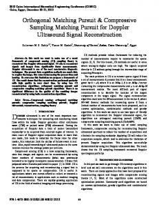
In this section, we identify conditions which guarantee that the Logit-GOMP algorithm does not select any wrong groups. The case of Logit-GOMP differs significantly from the “regular” Group-OMP due to the strongly non-linear characteristics of the operators involved, namely, due to the effects introduced by the link function g −1 . As a result, one should expect a non-linear set of conditions to be necessary to guarantee that the algorithm selects the correct feature groups and this is the case indeed. Nevertheless the set of conditions presented here have an elegant geometric character. Let Ggood denote the set of all the groups included in the true model, and let Gbad denote the set of all the groups which are not included. Similarly denote by ggood the set of feature indices for the features in the true model, and by gbad the set of feature indices for the features that are ¯ ⊆ ggood , not in the true model. In this notation supp(β) ¯ where β denote the true model coefficients. Define Θ(y) as } { Θ(y)= y ˜ : ∥˜ y∥ = 1 ∧ ∀i∈{1,...,n} sign(˜ yi ) = sign(yi − 21 ) ,

that is the intersection of an (n − 1)-dimensional unit sphere in Rn with the n-dimensional orthant containing the vector [sign(y1 − 12 ), sign(y2 − 12 ), . . . , sign(yn − 12 )]T . Analogously, for a set of vectors G let Λ(G)={˜ y : ∥˜ y∥ = 1∧

} ∀i∈{1,...,n} sign(˜ yi ) = sign(vi ), v ∈ spanG , An example for Θ(y) is depicted in Figure 3.2. 1.0

0.5

0.0 1.0

0.5

1

with the fact that if there exists r > 0 such that for all t, 1 ⌉, there holds ϵt+1 ≤ ϵt − rϵ2t , then for ϵ > 0 and k ≥ ⌈ rϵ ϵk ≤ ϵ (see [19] Appendix B Lemma B.2.).

≥

Variable Selection Accuracy

1

1 ≤ Q(ηβ ) + |G\G| inf α {α[Q(ηβ¯ ) − Q(ηβ )− ¯ ∑ ρ 1 2 2 ¯ ∥β¯Gi ∥21 }. ¯ Gi ∈G\G 2 ∥β − β∥2 ] + 8 α Optimizing for α, we obtain the lemma. Let ϵk = Q(ηβ (k) ) − Q(ηβ¯ ). Theorem 1 follows by noting that Lemma 1 with ρ = 0 (simple convexity assumption which holds by convexity of the logistic loss) leads to ϵ2 ∑ k ϵk+1 ≤ ϵk − 1 |G\G|∥ , and combining this ¯ ∥β¯ ∥2 ¯ 2

3.2

4ρ k ¯G ∥ ) . ¯ max |G| ¯ ∥β Gi ∈ G i 0

The theorem follows by using 1 − x ≤ exp(−x).

-0.5

0.0

Figure 2: The set Θ(y) in 3 dimensions for y = [1, 0, 1]T Theorem 3. Suppose that the design matrix X and the response vector y satisfy the following condition:

4ρϵk ¯G ∥ . ¯ max |G| ¯ ∥β Gi ∈ G i 0

By recursion we obtain ϵk ≤ ϵ0 (1 −

0.0 -1.0

sup ∥XTGj y ˜ ∥2
12 if and only if x > 0 and g −1 (x) < 12 if and only if x < 0 and the corollary follows. ∪ Intuitively, Θ(y) and Λ( Ggood ) capture the sub-space in which the (pseudo) residual vectors reside, given that the algorithm has not selected a wrong group up to that stage. For linear regression, the equivalent of Θ(y) happened to be the span of the “good” feature vectors, but here (for the non-linear case) they no longer coincide. Hence, the need arises to geometrically characterize a region in which the residuals will fall into, as long as the algorithm does not make any mistake, and make sure that the maximum projection onto this region is achieved by a “good” group. We remark that our results can be seen as the counterpart of Theorem 3.1 in [21] for OMP, and Corollary 1 in [11] for Group-OMP. Note that the conditions of (1) and (2) are similar in character to the (linear) condition for the GroupOMP (see definition and condition on quantity µX (Ggood ) in Corollary 1 of [11]). Sets Θ and Λ are nonlinear objects (as opposed to “regular” norms in cases of OMP and Group-OMP), which reflects the nature of the logistic setting. To the best of our knowledge, such “exact recovery” conditions had not been formulated before for matching pursuit techniques with models others than linear regression. An important direction for future research is a probabilistic analysis to bound the probability of observing a random sample for which the conditions are violated.

456

4 Experiments 4.1

Simulation Results

We empirically evaluate the performance of the proposed Logit-GOMP method against a number of comparison methods. The goal of Experiments 1 and 2 is to compare Logit-GOMP, Logit-OMP, Logistic Group Lasso, Logistic Lasso and Ordinary Logistic Regression (denoted by OLR). Logistic Group Lasso is included as a representative method of variable group selection, while comparison with Logit-OMP and Logistic Lasso will test the effect of “grouping”. Note that by Logit-OMP we denote the special case of Logit-GOMP with groups of size one. In Experiment 3, we focus more closely on the grouped methods, namely Logit-GOMP and Logistic Group Lasso, by comparing their performance on models involving two-way interactions and a much larger parameter space. We test how their performance changes when we vary the correlation between the predictors and the Bayes risk (in other words the difficulty of the classification task). In each experiment, we compare the performance of the competing methods in terms of the accuracy of variable selection, variable group selection and prediction accuracy. As measure of variable (group) selection accuracy we use R the F1 measure, which is defined as F1 = P2P+R , where P denotes the precision and R denotes the recall. For computing variable group F1 for a variable selection method, we consider a group to be selected if any of the variables in the group is selected. The measure of F1 for the variable group selection accuracy is analogously defined, where precision and recall are measured with respect to the variable groups, instead of individual variables. As measure of prediction accuracy, we use the test set negative log-likelihood. Recall that Logistic Group Lasso solves ] ∑ [ argminβ −

n i=1

yi ηβ (xi )−log(1 + eηβ (xi ) ) +λ

∑J

j=1∥βGj ∥2 ,

and Logistic Lasso solves the same problem under the special case where groups are individual features. So the tuning parameter for Logistic Lasso and Logistic Group Lasso is the penalty parameter λ. For Logit-GOMP and LogitOMP, rather than parameterizing the models according to precision ϵ, we use the iteration number as tuning parameter (i.e. a stopping point). Then for all methods we consider the “holdout validated estimate”, which is obtained by selecting the tuning parameter that minimizes the negative log-likelihood on on a validation set. We now describe the experimental setup. Recall that the empirical Bayes risk ∑nfor a model is rb = n1 i=1 min{pβ (xi ), 1 − pβ (xi )}, where pβ (xi ) denote the class conditional probability and n is large. For each observation xi , the response yi is simulated according to a Bernoulli distribution with probability pβ (xi ), where pβ (xi ) is defined in each experiment. For each experiment, we ran 100 runs, each with a training set


of size ntrain = 500, and validation set (for picking the tuning parameter for each method) of size nval = 500, and a test set of size ntest = 500. Experiment 1: categorical variables. We use an additive model with categorical variables obtained by adapting model I in [24] to the logistic regression setting. Consider variables z 1 , . . . , z 15 , where z j ∼ N (0, 1)(j = 1, . . . , 15) and cov(z j , z k ) = 0.5|j−k| . Let w1 , . . . , w15 be such that   0 if z j < Φ−1 (1/3) 1 if z j > Φ−1 (2/3) wj = ,  2 if Φ−1 (1/3) ≤ z j ≤ Φ−1 (2/3) where Φ−1 is the quantile function for the normal distribution. The true underlying model is ηβ (w) = 1.8I(w1 = 1) − 1.2I(w1 = 0) + I(w3 = 1)+ 0.5I(w3 = 0) + I(w5 = 1) + I(w5 = 0), where I denote the indicator function. Then we 2(j−1)+1 reparameterize the model and let (x , x2j ) = ( ) j j I(w = 1), I(w = 0) , which are the variables used as explanatory variables by the estimation method, with the following variable groups: Gj = {2j − 1, 2j}(j = 1, . . . , 15). The empirical Bayes risk is rb = 0.23. Experiment 2: continuous variables with polynomial expansion. We use an additive model with continuous variables obtained by modifying model III in [24] to the logistic regression setting. In this model, the groups correspond to the expansion of each variable into a third-order polynomial. . Consider variables z 1 , . . . , z 17 , with z j i.i.d. ∼ N (0, 1) (j = 1,√. . . , 17). Let w1 , . . . , w16 be defined as wj = (z i + z 17 )/ 2. The true underlying model is ηβ (w) = (w3 )3 + (w3 )2 + w3 + 13 (w6 )3 − (w6 )2 + 23 w6 . Then let the explanatory variables be ( ) (x3(j−1)+1 , x3(j−1)+2 , x3j ) = (wj )3 , (wj )2 , wj with the variable groups Gj = {3(j − 1) + 1, 3(j − 1) + 2, 3j}(j = 1, . . . , 16). The Bayes risk for this model is rb = 0.20. Experiment 3: Categorical variables with two-way interaction. We use the same simulation scheme as that of [14]. Consider variables z 1 , . . . , z 9 , where z i ∼ N (0, 1) and cov(z i , z j ) = ρ|i−j| , where ρ will be specified. Let w1 , . . . , w9 be such that  0 if z j < Φ−1 (1/4)    1 if Φ−1 (1/4) ≤ z j < Φ−1 (1/2) wj = , 2 if Φ−1 (1/2) ≤ z j < Φ−1 (3/4)    −1 j 3 if Φ (3/4) ≤ z where Φ−1 is the quantile function for the normal distribution. The encoding scheme for such categorical variables is dummy encoding with sum constraint [17]. Recall that a categorical predictor taking k possible values has k − 1 degrees of freedom. The vector βg corresponding the encoding of a predictor with dfg degrees of freedom is setup as

457

follows. Coefficients β˜g,1 , . . . , β˜g,df +1 are sampled from the distribution N (0, 1). These are then transformed as follows. ∑dfg +1 ˜ βg,k ,for j ∈ {1, . . . , dfg }. βg,j = β˜g,j − dfg1+1 k=1 The intercept β0 is set to 0. The whole vector β is subsequently rescaled according to a desired value of the empirical Bayes risk. For each model below and values of ρ and rb , the true model coefficient vector β is then held fixed and data is simulated accordingly for each simulation run. We consider the following underlying models: Model A The true model is made from the main effects and two-way interaction between the first two factors x1 and x2 . Thus it involves J = 4 terms (Intercept, x1 , x2 , x1 x2 ) implying a dummy encoding of p = 16 parameters. Model B The true model is made from the main effects and two-way interaction between the first five factors x1 , . . . , x5 . Thus it involves J = 16 terms (Intercept, x1 , x2 , x3 , x4 , x5 , x1 x2 , x1 x3 , x1 x4 , x1 x5 , x2 x3 , x2 x4 , x2 x5 , x3 x4 , x3 x5 , x4 x5 ) implying a dummy encoding of p = 106 parameters. The candidate models are those with the main effects and two-way interactions for all the 9 variables, which involves J = 46 terms or p = 352 parameters. For each model, we study rb ∈ {0.15, 0.25} and ρ ∈ {0.20, 0.50}. The results of Experiments 1 and 2 are presented in Table 1. The results of Experiments 3, Model A are presented in Table 2, and those for Model B in Table 3. We note that F1 (Var) and F1 (Group) are identical for the grouped methods for Experiments 1, 2 since in these the groups have equal size. Overall, Logit-GOMP performs consistently better than all the comparison methods, with respect to all measures considered. In particular, Logit-GOMP does better than Logit-OMP not only for variable group selection, but also for variable selection and predictive accuracy. Consistently to what was noted in [14], we observe that Logistic Group Lasso has a tendency to over-select (groups of) variables, leading to poorer F1 measure, while Logit-GOMP is more parsimonious and accurate. This becomes more pronounced when the true model gets sparser (e.g. Experiment 3, Model B vs. Experiment 3, Model A). Also LogitGOMP is at least competitive to Logistic Group Lasso with respect to negative log-likelihood minimization. We remark that the negative log-likelihood values we got for Logistic Group Lasso in Experiments 3 are consistent with what have been reported in the literature [14]. 4.2

Experiments on Splice Site Detection

In this section, we compare Logit-GOMP and Logistic Group Lasso using the MEMset donor data set [23] on splice site detection (available at http://genes.mit.edu/burgelab/maxent/ssdata/). Splice sites detection is a critical prerequisite to gene iden-


F1 (Var) Ordinary Logistic Regression Logistic Lasso Logit-OMP Logistic Group Lasso Logit-GOMP

Exp 1 0.333 ± 0 0.547 ± 0.032 0.851 ± 0.027 0.494 ± 0.035 0.896 ± 0.037

Exp 2 0.222 ± 0 0.371 ± 0.011 0.629 ± 0.0251 0.312 ± 0.0181 0.990 ± 0.010

F1 (Group) Ordinary Logistic Regression Logistic Lasso Logit-OMP Logistic Group Lasso Logit-GOMP

Exp 1 0.333 ± 0 0.463 ± 0.033 0.845 ± 0.038 0.494 ± 0.035 0.896 ± 0.037

Exp 2 0.222 ± 0 0.311 ± 0.019 0.873 ± 0.031 0.312 ± 0.0181 0.990 ± 0.010

Negative log-likelihood Ordinary Logistic Regression Logistic Lasso Logit-OMP Logistic Group Lasso Logit-GOMP

Exp 1 248.38 ± 2.42 237.17 ± 2.09 237.08 ± 2.45 236.25 ± 2.08 236.06 ± 2.40

Exp 2 237.23 ± 4.64 207.87 ± 2.86 207.26 ± 3.44 207.70 ± 2.86 196.73 ± 2.96

Table 1: Results of Experiment 1 and Experiment 2: Average F1 score at the variable level and group level (higher value is better), and negative log-likelihood (summed over test set; lower value is better) for the models output by Ordinary Logistic Regression, Logistic Lasso, Logit-OMP, Logistic Group Lasso, and Logit-GOMP. F1 Logistic Group Lasso Logit-GOMP

ρ = 0.5, rb = 0.25 0.247 ± 0.078 0.878 ± 0.011

ρ = 0.5, rb = 0.15 0.318 ± 0.033 0.890 ± 0.021

ρ = 0.20, rb = 0.25 0.76 ± 0.019 0.880 ± 0.014

ρ = 0.20, rb = 0.15 0.307 ± 0.021 0.890 ± 0.022

F1 (Group) Logistic Group Lasso Logit-GOMP

ρ = 0.5, rb = 0.25 0.355 ± 0.010 0.793 ± 0.023

ρ = 0.5, rb = 0.15 0.406 ± 0.036 0.800 ± 0.006

ρ = 0.20, rb = 0.25 0.309 ± 0.0233 0.793 ± 0.026

ρ = 0.20, rb = 0.15 0.383 ± 0.0222 0.938 ± 0.013

Negative log-likelihood Logistic Group Lasso Logit-GOMP

ρ = 0.5, rb = 0.25 258.76 ± 9.42 249.75 ± 9.49

ρ = 0.5, rb = 0.15 184.58 ± 2.12 181.92 ± 5.46

ρ = 0.20, rb = 0.25 274.81 ± 2.18 272.91 ± 2.48

ρ = 0.20, rb = 0.15 187.58 ± 2.45 193.246 ± 3.53

Table 2: Results of Experiment 3 Model A: Average F1 score at the variable level and group level (higher value is better), and negative log-likelihood (summed over the test set; lower value is better) for the models output by Logistic Group Lasso and Logit-GOMP. F1 Logistic Group Lasso Logit-GOMP

ρ = 0.5, rb = 0.25 0.571 ± 0.007 0.534 ± 0.033

ρ = 0.5, rb = 0.15 0.553 ± 0.008 0.633 ± 0.021

ρ = 0.20, rb = 0.25 0.577 ± 0.010 0.600 ± 0.030

ρ = 0.20, rb = 0.15 0.546 ± 0.006 0.686 ± 0.024

F1 (Group) Logistic Group Lasso Logit-GOMP

ρ = 0.5, rb = 0.25 0.598 ± 0.007 0.496 ± 0.014

ρ = 0.5, rb = 0.15 0.5856 ± 0.008 0.5934 ± 0.020

ρ = 0.20, rb = 0.25 0.615 ± 0.010 0.695 ± 0.026

ρ = 0.20, rb = 0.15 0.576 ± 0.006 0.578 ± 0.021

Negative log-likelihood Logistic Group Lasso Logit-GOMP

ρ = 0.5, rb = 0.25 294.78 ± 1.76 293.06 ± 2.40

ρ = 0.5, rb = 0.15 235.16 ± 4.08 236.92 ± 6.14

ρ = 0.20, rb = 0.25 308.70 ± 2.07 307.48 ± 3.02

ρ = 0.20, rb = 0.15 234.73 ± 2.45 234.20 ± 2.31

Table 3: Results of Experiment 3 Model B: Average F1 score at the variable level and group level (higher value is better), and negative log-likelihood for the models (summed over the test set; lower value is better) output by Logistic Group Lasso and Logit-GOMP.

458

Group Orthogonal Matching Pursuit for Logistic Regression Method Logistic Group Lasso Logit-GOMP

Maximal correlation coefficient 0.6588 0.6591

Table 4: Maximal correlation coefficients for Logistic Group OMP and Logistic Group Lasso on the splice site detection data.

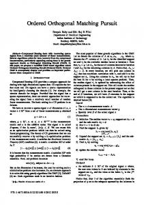
Figure 3: Normalized l2 -norms ∥βGj ∥/∥β∥, j = 1, . . . , J for the estimated models produced by Logit-GOMP and Logistic Group Lasso for the splice site detection problem.

tification in genomic DNA. These sites are the regions between exons (coding) and introns (non-coding) DNA segments. The 5’ boundary of an intron, also called donor splice site starts with the dinucleotide ‘GT’, and the 3’ boundary of an exon, also called acceptor splice site contains the dinucleotide ’AG’ (see [3] for more details). Several computational methods have been developed for detecting splice sites [2, 23, 16].

groups, and p = 211 variables. As measure of performance, we used the “maximum ∑ntest coefficient” ρmax defined as: ρmax = maxα∈(0,1) { i=1 (yi (I(pβ (xi ) > α)))}. The results are provided in Table 4. Figure 4 depicts the normalized l2 -norm of the regression coefficients for the groups, as estimated by the two competing methods. Notice from the figure that Logit-GOMP and Logistic Group Lasso grant similar importance to a majority of groups and that the model output by Logit-GOMP is sparser. In view of these results, we conclude that on this high dimensional problem, Logit-GOMP is at least competitive with Logistic Group Lasso, as well as with the results of [23], where ρmax = 0.6589 was achieved.

5

Concluding Remarks and Perspectives

The MEMset donor data set consists of “real splice site” and “false splice site” instances. A “real splice site” consists of the last three bases of the exon and the first six bases of the intron, and hence, contains ‘GT’ at positions 4 and 5. A “fast splice site” also contains those letters at positions 4 and 5 but is not an actual splice site. After removal of the common letters ‘GT’ at positions 4 and 5, the predictor variables are thus sequences of 7 bases, where each base takes value in {A, C, G, T } while the target is binary: Y = 1 for “false splice sites” and Y = 0 for true ones.

By proposing a generic matching pursuit method for variable group selection in generalized linear models, and demonstrating its competitive performance for logistic regression, we are opening up a research agenda on the consideration and analysis of matching pursuit techniques as competitive alternatives to l1 penalized regression methods, for a variety of models beyond linear regression.

We follow the experimental setup of [14]. Namely, we build a balanced training set with 5610 positive and 5610 negative instances, using the original training set, as well as an unbalanced validation set with 2850 positive and 59804 negative instances (with same class ratio as that in the test set). The instances are randomly sampled without replacement, and hence training and evaluation sets do not intersect. We use the original test set as is. We perform intercept correction to account for the difference in class-ratio between training and (validation sets as: ) Number of true sites in validation set β0adj = β0 + log Number of false sites in validation set .

In view of the recent results of [4, 26], the discrepancies between the theoretical guarantees for Lasso and OMP obtained so far are very narrow and subtle. A very pertinent direction for future investigation is thus to theoretically and experimentally characterize precise settings where one type of method would perform better than the other.

The stopping point of Logit-GOMP and the penalty parameter for Logistic Group Lasso are chosen so as to minimize the negative log-likelihood on the validation set using estimated models with corrected intercept. We use as candidate model a logistic regression model with all main effects and two way interactions (it was noted in [14] that considering up to three way interactions gives similar results). We thus consider J = 28

459

Relevant directions for future research include extending our theoretical analysis to the stochastic setting, and proving performance guarantees for other instances of our generic algorithm under generalized linear models.

We also plan to apply the proposed method in a variety of problems in which variable group selection involving both continuous and categorical variables is important, such as modeling from time series data with mixed data types. Acknowledgements Research supported through participation in the Measurement Science for Cloud Computing, sponsored by the National Institute of Standards and Technology (NIST) under Agreement Number 60NANB10D003.


References [1] BACH , F.R., Consistency of the Group Lasso and Multiple Kernel Learning, J. Mach. Learn. Res., 9, 1179-1225, 2008. [2] B URGE , C. AND K ARLIN , S., Prediction of complete gene structures in human genomic DNA., J. Molec. Biol., 268, 7894, 1997. [3] B URGE , C., Modeling dependencies in pre-mrna splicing signals. In Computational Methods in Molecular Biology (eds S. Salzberg, D. Searls and S. Kasif), ch. 8, pp. 129164. New York: Elsevier Science. 1998. [4] F LETCHER A., R ANGAN S., Orthogonal Matching Pursuit From Noisy Random Measurements: A New Analysis, in proc. NIPS’09, 2009. [5] F REUND . Y., S CHAPIRE , R. E., A decision-theoretic generalization of on-line learning and an application to boosting, Journal of Computer and system Sciences, Vol. 55(1), 119-139, 1997. [6] F RIEDMAN J., H ASTIE T., T IBSHIRANI R., Additive Logistic Regression: a Statistical View of Boosting. Technical report, Department of Statistics, Stanford University, 1998. [7] H ASTIE T., T IBSHIRANI R., F RIEDMAN J., The Elements of Statistical Learning: Data Mining, Inference, and Prediction, Springer, 2003. [8] H UANG J., Z HANG T., M ETAXAS D., Learning with Structured Sparsity, in ICML’09, 2009. [9] K AKADE S., S HAMIR O., S RIDHARAN K., T EWARI S., Learning Exponential Families in High Dimensions: Strong Convexity and Sparsity, AISTATS 2010. [10] K IM Y., K IM J., K IM Y., Blockwise sparse regression, Statistica Sinica, 16, 375–390, 2006. [11] L OZANO A.C., S WIRSZCZ G., A BE N., Grouped Orthogonal Matching Pursuit for Variable Selection and Prediction,in proc. NIPS’09, 2009. [12] M ALLAT S., Z HANG Z., Matching pursuits with time-frequency dictionaries, IEEE Transactions on Signal Processing, 41, 3397-3415, 1993. [13] M ASON L., BAXTER J., BARTLETT P., F REAN M., Boosting Algorithms as Gradient Descent, in Neural Information Processing Systems, Vol. 12, pp. 512518, 2000. ¨ P., The [14] M EIER L., VAN DE G EER , S., B UHLMANN group lasso for logistic regression, J. Royal Statistical Society: Series B, 70(1), 53-71, 2008.

460

[15] ROCHA G., WANG X., Y U B., Asymptotic distribution and sparsistency for l1 penalized parametric Mestimators, with applications to linear SVM and logistic regression, Technical report, 2009 [16] M. P ERTEA , X. L IN , S. L. S ALZBERG, GeneSplicer : a new computational method for splice site prediction Nucleic Acids Res, 29(5), 1185-90, 2001 [17] Q UINN , G ERALD P ETER , AND K EOUGH , M ICHAEL, J. Experimental design and data analysis for biologists, Cambridge University Press, 2002 [18] ROTH V., F ISCHER B. The Group-Lasso for generalized linear models: uniqueness of solutions and efficient algorithms. In Proceedings of the 25th ICML conference (ICML’08), 307, 848-855, 2008. [19] S HALEV-S HWARTZ S., S REBRO N., Z HANG T., Trading Accuracy for Sparsity, Technical Report TTIC-TR-2009-3, May 2009. [20] T IBSHIRANI , R., Regression shrinkage and selection via the lasso, J. Royal. Statist. Soc B., 58(1), 267-288, 1996. [21] T ROPP J.A., Greed is good: Algorithmic results for sparse approximation, IEEE Trans. Info. Theory, 50(10), 2231-2242, 2004. [22] V INCENT P., B ENGIO Y., Kernel matching pursuit, Machine Learning, 48. 165–187, 2002. [23] Y EO , G. W. AND B URGE , C. B., Maximum entropy modeling of short sequence motifs with applications to RNA splicing signals. J. Computnl Biol., 11, 475494, 2004. [24] Y UAN , M., L IN , Y., Model selection and estimation in regression with grouped variables, J. R. Statist. Soc. B, 68, 4967, 2006. [25] Z HANG , T., On the consistency of feature selection using greedy least squares regression, J. Machine Learning Research, 2008. [26] Z HANG , T., Sparse Recovery with Orthogonal Matching Pursuit under RIP, Tech Report arXiv:1005.2249, 2010. [27] Z HAO , P, ROCHA , G. AND Y U , B., Grouped and hierarchical model selection through composite absolute penalties, Manuscript, 2006. [28] Z OU , H., H ASTIE T., Regularization and variable selection via the Elastic Net., J. R. Statist. Soc. B, 67(2) 301-320, 2005.