H-CNNs: Convolutional Neural Networks for Riemannian ...

H-CNNs: Convolutional Neural Networks for Riemannian Homogeneous Spaces Rudrasis Chakraborty† , Monami Banerjee† and Baba C. Vemuri Department of CISE, University of Florida, FL 32611, USA

∗

arXiv:1805.05487v1 [cs.CV] 14 May 2018

† Equal Contribution

{rudrasischa, monamie.b, baba.vemuri}@gmail.com

Abstract Convolutional neural networks are ubiquitous in Machine Learning applications for solving a variety of problems. They however can not be used as is when data naturally reside on commonly encountered manifolds such as the sphere, the special orthogonal group, the Grassmanian, the manifold of symmetric positive definite matrices and others. Most recently, generalization of CNNs to data residing on a sphere has been reported by some research groups, which go by several names but we will refer to them as spherical CNNs (SCNNs). The key property of SCNNs distinct from the standard CNNs is that they exhibit the rotational equivariance property. In this paper, we theoretically generalize the SCNNs to Riemannian homogeneous manifolds, that include many commonly encountered manifolds including the aforementioned example manifolds. Proof of concept experiments involving synthetic data generated on the manifold of (3 × 3) symmetric positive definite matrices and the product manifold of R+ × S2 respectively, are presented. These manifolds are commonly encountered in diffusion magnetic resonance imaging, a non-invasive medical imaging modality.

1

Introduction

Convolutional neural networks introduced by Lecun [17] have gained enormous attention in the past decade especially after the demonstration of the signifi cant success on Imagenet data by Krizhevsky et al. [16] and others. The key property of equivariance to translation of patterns in the image is utilized in the CNN to share weights across the network and achieve efficiency. Thus, one might consider exploiting equivariance to transformation groups as a key design principle in designing neural network architectures suitable for these groups. For data sets that reside on Riemannian manifolds, it would then be natural to seek a symmetry group property that the manifold admits and define the convolution operation on the manifold that would be equivariant to this symmetry group. For instance, on the n-sphere, the natural group action is the rotation group i.e., moving from one point on the n-sphere to another point can be achieved via a rotation. Rotations in n-dimensions are elements of the well known group called ∗ This

research was funded in part by the NSF grant IIS-1525431 and IIS-1724174 to BCV.

1

the special orthogonal group, SO(n), which is a Lie group [13]. Thus, to develop convolution of functions on the sphere, we seek equivariance with respect to rotations. This way, we will have the flexibility to seek filters/masks that are orientation sensitive. Steerability of filters has been recognized as being of great importance in Computer Vision literature several decades ago in context of hand crafted features [12, 7, 19]. Steerability here refers to reconstruction of all deformations (scale, rotation and translation) of the filter using a small number of basis functions. Most recently, steerable CNNs have been reported in literature [8, 6, 5] that can cope with data residing on a 2-sphere and hence are equivariant with respect to rotations in 3D i.e., SO(3). In another recent work [9], authors describe what they call polar transformer networks, which are equivariant to rotations and scaling transformations. By combining them with what is known in literature as a spatial transformer [15], they achieve the required equivariance to translations as well. In this paper, we present a novel generalization of group convolution equivariance property to homogenous Riemannian manifolds. Very simply said, a homogeneous Riemannian manifold for a group G is a nonempty topological space M on which G acts transitively [14]. The elements of G are called symmetries of M. Intuitively, a homogeneous space, a.k.a. a homogeneous Riemannian manifold, is one which ‘looks” the same locally at all points on it with respect to some geometric property such as isometry, diffeomorphism etc. Some important examples of homogeneous spaces include Riemannian symmetric spaces e.g., the n-sphere (Sn ), projective space, euclidean space, the Grassmanian, manifold of (n, n) symmetric positive definite matrices denoted by Pn , and others. Most of these manifolds are commonly encountered in mathematical formulations of various Computer Vision tasks such as action recognition, covariance tracking etc. and in Medical Imaging for example in dMRI, elastography, conductance imaging etc. By providing a general framework suited for manifold-valued data sets, that is analogous to the CNNs, in this paper, we extend the success of CNNs to several high dimensional yet unexplored input data domains. We present two sets of synthetic experiments to demonstrate the performance of our theoretical framework that we will henceforth call, the H-CNN for homogenous space CNN. In the first experiment, we take two classes consisting of functions on the (3 × 3) symmetric positive definite matrices, P3 . The functions are Gaussian distributions on P3 , for simplicity, we assumed these Gaussian distributions to be of unit variance but distinct means. We classify samples from these two classes of distributions using our proposed H-CNN framework. In our second experiment, we generated diffusion magnetic resonance imaging (dMRI) data synthetically. The dMRI data was generated from three distinct spatial arrangement of diffusion profiles, a circular pattern with and without diagonal crossing spokes and a third, which is a sinusoidal pattern. We can view each dMRI sample from any of the above three classes as a function on the homogeneous space R+ × S2 . Then, we classify these three classes using our proposed H-CNN. Finally, we present a real data experiment involving a classification of dMRI scans acquired from a cohort of 41 Parkinson Disease patients and 50 Control subjects. We first compute the ensemble average propagator (EAP), a probability density function P (r) from the raw dMRI data. The EAP quantifies the probability of a water molecule moving along the radial vector r ∈ R3 . The EAP is known to fully capture the diffusional characteristics locally 2

at a voxel in the image lattice. Under the short pulse assumption, EAP is related to the raw diffusion sensitizedR magnetic resonance (MR) signal, S(q), via the 3D Fourier transform P (r) = S(q) exp 2πjqt rdr [3]. We represent each EAP as a function on the product manifold, R+ × S 2 . This provides us the data in the form discussed earlier. In all of our experiments, we have shown reasonably good classification accuracy using our proposed H-CNN framework. In summary, our key contributions in this paper are: (i) We present a nontrivial theoretically consistent generalization of CNNs to cope with data residing in Riemannian homogeneous spaces which are often encountered both in computer vision and medical imaging applications. (ii) We present proof of concept experiments on synthetic data on the space of (3 × 3) symmetric positive definite matrices, P3 , and on synthetically generated dMRI data represented as samples of functions on the product manifold, R+ × S2 . Rest of the paper is organized as follows. In section 2 we present the main theoretical result showing the equivariance of convolution on homogeneous spaces. Following this, we apply this theorem to the case of product manifold of R+ × S2 used to naturally represent dMRI data. Then we present the setting for the homogeneous space of non-compact type namely, P3 . Section 2 contains a detailed description of the proposed H-CNN architecture. In section 3 we present the experimental results and conclude in section 4.

2

Correlation on Riemannian homogeneous spaces

In this section, first we present a brief note on the differential geometry of Riemannian homogeneous spaces required in the rest of the paper. For a detailed exposition on these concepts, we refer the reader to a comprehensive and excellent treatise on this topic by Helgason [14]. Preliminaries. Let (M, g M ) be a Riemannian manifold with a Riemannian metric g M , i.e., (∀x ∈ M) gxM : Tx M × Tx M → R is a bi-linear symmetric positive definite map, where Tx M is the tangent space of M at x ∈ M. Let d : M × M → R be the metric (distance) induced by the Riemannian metric g M . Let I(M) be the set of all isometries of M, i.e., given g ∈ I(M), d(g.x, g.y) = d(x, y), for all x, y ∈ M. It is clear that I(M) forms a group (henceforth, we will denote I(M) by G) and thus, for a given g ∈ G and x ∈ M, g.x 7→ y, for some y ∈ M is a group action. Since we choose the left group action, we will denote it by Lg , i.e., Lg (x) = g.x. Note that Lg : M → M is a diffeomorphism. Consider o ∈ M, and let H = Stab(o) = {h ∈ G|h.o = o}, i.e., H is the Stabilizer of o ∈ M. We say that G acts transitively on M, iff, given x, y ∈ M, there exists a g ∈ M such that y = g.x. Definition 1 (Riemannian homogeneous space). Let G = I(M) act transitively on M and H = Stab(o), o ∈ M (called the “origin” of M) be a subgroup of G. Then, M is a homogeneous space and can be identified with the quotient space G/H under the diffeomorphic mapping gH 7→ g.o, g ∈ G [14]. Below, we list some of the properties of Riemannian homogeneous spaces that we will need in the rest of the paper. With a slight abuse of notation, we will use the term, homogeneous space, to denote a Riemannian homogeneous space i.e., that the homogeneous space is endowed with a Riemannian metric.

3

Properties of Homogeneous spaces: Let (M, g M ) be a Homogeneous space. Let ω M be the corresponding volume density and f : M → R be any integrable function. Let g ∈ G, s.t. y = g.x, x, y ∈ M. Then, the following facts are true: 1. g M (dy, dy) = g M (dx, dx). 2. d(x, z) = d(y, g.z), for all z ∈ M. Z Z M 3. f (y)ω (x) = f (x)ω M (x) M

M

Because of property 1, the volume density is also preserved by the transformation x 7→ g.x, for all x ∈ M and g ∈ G. Now, we will give the principal bundle structure of the homogeneous space which we will need in this paper. Proposition 1. The homogeneous space, M identified as G/H together with the projection map Π : G → G/H is a principal bundle with H as the fiber. In order to define the correlation of two functions, we will first define the pushforward of a function and then define the correlation based on the pushforward function. Note that we will need the correlation operation in defining our deep network architecture subsequently. Pushforward of a function f using a diffeomorphism φ: Let φ : M → N be a diffeomorphism between manifold M and N . Let f : M → R be a function on M. We can define the pushforward of f by φ denoted by φ∗ f : N → R as y 7→ f (φ−1 (y)). Since φ is a diffeomorphism φ−1 exists and φ−1 (y) ∈ M and hence φ∗ f is a function from N to R. Equipped with the above definitions, we are now ready to formally define the correlation of two L2 (square integrable) functions f : M → R and w : M → R. We will assume M to be a homogeneous space for the rest of the paper if not mentioned otherwise. We will also assume that G is the group of isometries acting transitively on M. Definition 2 (Correlation). Using the above notations, the correlation between f and w is given by, (f ? w) : G → R as follows: Z (f ? w) (g) := f (x) (Lg∗ w) (x)ω M (x) (1) M

Below, we discuss and prove some of the properties of the above defined correlation operation. The main property is that the correlation operation defined above is equivariant with respect to the group action defined on M. We will first define some terminologies to prove the equivariance. Definition 3 (G set). Let S = {f : M → R}. G acts on S as follows: g.f = Lg∗ f . Hence, S is a G set. Proposition 2. Let w ∈ S. Let U = {(f ? w) : G → R|f ∈ S}. Then, U is a G set. Proof. Since g. (f ? w) is a valid group action, hence U is a G set.

4



Now, we will prove that the above definition of correlation is equivariant. The equivariance is an important property of correlation/ convolution which is needed to ensure that the extracted features, i.e., output of the correlation operation, are “shifted” by the same amount as the input. Note that the term “shift” here refers to the appropriate group action. We will first formally define equivariance and then prove the equivariance property. Note that earlier works have presented this on Lie groups but not on Riemannian homogeneous spaces, which are more general but yet widely encountered in Medical Imaging and Computer Vision applications among others. Definition 4 (Equivariance). Let X and Y be G set. Then, F : X → Y is said to be equivariant if F (g.x) = g.F (x)

(2)

for all g ∈ G and all x ∈ X. Theorem 1. Let F : S → U be a function given by f 7→ (f ? w). Then, F is equivariant. Proof. We have to check if Definition 4 is satisfied. Let g, h ∈ G and f ∈ S.Then, (F (g.f )) (h) = (g. (f ? w)) (h) = (Lg∗ f ? w) (h) Z
= (Lg∗ f ) (x) Lh∗ w (x)ω M (x) ZM
= f (y)w (h−1 g).y ω M (y) M
= (f ? w) g −1 h = Lg∗ (f ? w) (h) = (Lg∗ F (f )) (h) = (g.F (f )) (h) Since, g, h ∈ G and f ∈ S are arbitrary, hence, Definition 4 is satisfied, i.e., F is equivariant.  Since S is a G set, hence, the definition of correlation in Definition 2 is analogous to the cross correlation of two functions on Euclidean space. This is because, (Lg∗ w) is the group action g.w for w ∈ S. Since we have shown the equivariance property and have a well-defined correlation operator, we can now think about cascading these correlation operations. In order to achieve this, we will need a definition of the correlation on G as (f ? w) : G → R and an appropriate non-linearity in between two layers. Note that, the definition of correlation in Definition 2 is valid if we have
M = G. In this situation, f, w : G → R and for h ∈ G, Lg∗ w (h) = w g −1 h . This leads us to the following corollary. Corollary 1. Let V = {f : G → R}. Let f, w ∈ V . Then, 1. (f ? w) : G → R is well-defined. 2. W = {(f ? w) : G → R|f ∈ V } is a G set. 5

3. F¯ : V → W given by f 7→ (f ? w) is equivariant. Proof. The first two claims follow from Definition 2 and 3. The last claim is an easy corollary of Theorem 1. 

2.1

Basis functions for L2 -functions on homogeneous spaces

Now, we will discuss the implementation of the above defined correlation in terms of a basis for square integrable functions on a Riemannian homogeneous space. In order to achieve this, we will first define the vector space of real-valued square integrable functions and define an inner product on this space. Let us denote the set of real-valued square integrable functions on M as L2 (M, R). Note that the integral is defined using the volume density induced from the Riemannian metric of M. Let, f, w ∈ L2 (M, R), then the inner product h, i : L2 (M, R) × L2 (M, R) → R is given by: Z hf, wi := f (x)g(x)ω M (x) (3) M

Proposition 3. L2 (M, R) is a vector space. Equipped with a well-defined correlation operation on M, now we will move on to discuss the choice of basis for L2 (M, R). 2.1.1

Basis on L2 (M, R) induced from L2 (G, R)

Analogous to Proposition 3, L2 (G, R) is also a vector space. Let {vα : G → R} be the set of basis of L2 (G, R). Using the principal bundle structure of the homogeneous space, we will get a set of basis on L2 (M, R) as follows: Proposition 4. {e vα : M → R} are linearly independent where, ve = ve π , where π e(x) = g if and only if x = π(g). Proof. Let us assumeP that, {e vα } are not linearly independent,P i.e., ∃ {cα } not all zero, such that, c v e (x) = 0 for all x ∈ M. Now, cα veα (x) = 0 α α P P =⇒ c α vα π e (x) = 0 =⇒ cα vα (g) = 0. The last equality holds for all g ∈ G such that, x = P π(g). As the above equations are true for all x ∈ M, it cα vα (g) = 0. As, ∃ {cα } not all zero, {vα } is linearly implies that ∀g ∈ G, dependent, which is a contradiction of our hypothesis. Note that, the above argument is true because M can be identified with G/H.  Proposition 5. {e vα } as defined above span L2 (M, R). Proof. It is enough to show that for all fe ∈ L2 (M, R), there exists f ∈ L2 (G, R) such that, fe = f ◦ π e. Now, Z  Z 2 2 M e f (x) ω (x) = (f ◦ π e(x)) ω M (x) M M Z 2 = (f (g)) ω M (π(g)) π(G) Z 2 = (f (g)) ω G (g) G

6

Here, ω G is the pull back measure on G by π, i.e., ω G := π ∗ ω M . As,



R M

fe(x)

2

∞, hence, f ∈ L2 (G, R).

ω M (x)
3, they are undefined. For L2 functions on SO(n) (with arbitrary n), one can use the Peter-Weyl’s basis [20], which by the Peter-Weyl’s theorem is the orthogonal Fourier basis for SO(n). But, unfortunately computation of these basis is infeasible, hence in this work, we propose a set of orthogonal basis induced from the Lie algebra, so(n) using the Cayley transform [13]. The Cayley −1 transform is a function Cay : so(n) → SO(n) defined as X 7→ (I − X) (I + X). −1 The inverse of the Cayley map is given by g 7→ (g − e)(g + e) . As, so(n) is the set of skew-symmetric matrices, (I − X) is invertible. Let ω so be the volume density on so(n). Now, as so(n) is a vector space, we can have a set of orthogonal basis, {vα }, on it (with respect to so(n)). We will use the push forward measure on SO(n) , denoted by ω SO , using Cay as
−1 SO so so ω (g) = Cay∗ ω (g) = ω Cay (g) . We can easily show that the push forward basis {e vα := Cay R ∗ vα } is mutuallySOorthogonal with respect to the push forward density, i.e., SO(n) veα (g)e vβ (g)ω (g) = 0, for all α 6= β. This gives us a easily computable mutually orthogonal basis on SO(n) for all n, which we can use to compute the correlations on higher dimensional homogeneous groups defined earlier. Orthogonal basis for L2 -functions on GL(n) and Pn : For L2-functions on a general linear group, GL(n), we have the orthogonal basis as proposed in [11]. On Pn , i.e., the space of symmetric positive definite matrices, one can use the Helgason-Fourier transformation [23] and use the orthogonal basis. But, as these are computationally (infeasible) expensive, we will use the parametrization using spectral decomposition, i.e., use the orthogonal matrix R and the diagonal matrix ⊕n D from RDRT . Hence, we will parametrize Pn by SO(n) × (R+ ) × Rn(n−1)/2 . On this parameter space, we will use the orthogonal basis on SO(n) and Laguerre polynomials [21] as basis on R+ . The correlation of functions on R+ is given below. Proposition 7. Given f, w : R+ → R, the correlation operation (f ? w) : R \ {0} → R is given by: Z (f ? w) (x) = f (y)w(x2 y)dy R+

Proof. The proof relies on fact that on Lx : R+ → R+ is given by y 7→ x2 y.  Orthogonal basis for L2 -functions on Sn−1 : We can use the induced basis on Sn−1 from SO(n) based on the construction described earlier. But 8

instead, we will use spherical harmonics to be our orthogonal basis functions as these are easily computable.

3

Experiments

IAs proof of concept, in this section, we present two sets of synthetic experiments namely, (i) synthetic data consisting of 2 classes synthesized from two distinct Gaussian distributions on P3 and (ii) synthesized dMRI data consisting of three classes having distinct diffusion profiles.

3.1

Classification from dMRI synthetic data

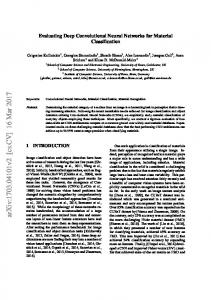
Diffusion MRI is a non-invasive diagnostic imaging technique that allows one to infer the axonal connectivity within the imaged tissue by sensitizing the MR signal to water diffusion in imaged tissue [2]. This is achieved via the application of magnetic field gradients over a sphere of directions. As of today, dMRI is the unique noninvasive technique capable of quantifying the anisotropic diffusion of water molecules in tissues allowing one to draw inference about neuronal connections between different regions of the central nervous system. In diffusion MRI, most applications rely on the fundamental relationship between the MR signal measurement S(q) and the average particle displacement density function (also known the ensemble average propagator or EAP) P (r) at a voxel, x = (x, y, z)tR, which is given by the following Fourier transform relationship [3]: S(q) = S( 0) R3 P (r) exp (iq · r) d(r) where S( 0) is the signal in the absence of any diffusion gradient, r is the displacement vector and r = γδGg, where γ is the gyromagnetic ratio, δ is the diffusion gradient duration, and G and g are the magnitude and direction of the diffusion sensitizing gradients respectively. There are numerous articles in literature on diffusion MR imaging and we refer the reader to [24] for details on the imaging method called high angular resolution diffusion imaging (HARDI) that is widely used in most dMRI acquisitions and here in our real data experiment. As mentioned earlier, the HARDI protocol used to acquire the dMRI data results in several 3D MR images, one each along the diffusion sensitizing magnetic field direction g described above. The natural mathematical space for describing the data domain for S(q) as well as the EAP, P (r), is S2 × R+ . In this experiment, we generated 24 × 24 dMRIs from three distinct spatial arrangements EAPs, a sinusoidal pattern and a circular pattern with and without diagonally crossing spokes (example samples without noise are shown in Figure 1). We generate 500 samples corrupted with Rician noise (ranging over SNRs 25-30) from each of these three classes and then use the H-CNN on this data to perform the classification. Network architecture for dMRI data: Note that the dMRI signal magnitude is a positive real number acquired along each magnetic field direction over a hemi-sphere of directions in 3D. As each sample of the data is a function f : S2 × R+ → R, we will use the well known SHORE basis [18, 10] to represent each function. The SHORE basis is a product of the spherical harmonic basis on S2 and the Laguerre polynomials on the radial component, i.e., on R+ . Recently, in [9], authors proposed a polar CNN on SO(2) × R+ . Though, one can use their framework in our application, we like to point out that they used a polar chart on SO(2) along with a log map on R and then used a standard CNN in this

9

Figure 1: Samples without noise from three distinct classes of the synthetic dMRI data. parameter space. This formulation is equivalent to the Log-Euclidean framework [1] and leads to inaccuracies when data variance is large. Now, we design an architecture for this product space representation, S2 ×R+ 2 where on S2 , we have CorrS → BN → SO(3)-ReLU → CorrSO(3) → BN → SO(3)-ReLU → CorrSO(3) → BN → SO(3)-ReLU. + On R+ , we have CorrR → Maxpool → BN → R \ {0}-ReLU → CorrR\{0} → Maxpool → BN → R \ {0}-ReLU → CorrR\{0} → Maxpool → BN → R \ {0}-ReLU. Here, BN is the Batch normalization step. Now, at the end we combine the two network outputs and add the BN, two FC layers with ReLU in between and a softmax layer at the end to perform classification of the data. In order to implement the convolution efficiently, we use the spherical harmonics as basis on S2 and the Cayley map induced basis on SO(3). On R+ , we use Laguerre polynomials as basis. In order to perform correlation on R \ {0}, and to make sure the output is on R \ {0}, we use ReLU such that the minimum value is  for a small enough . In this experiment, our implementation of the H-CNN yielded a training accuracy of 91.1% and a testing accuracy of 83.3% using a ten-fold partition of the data. We believe that a higher testing accuracy can be achieved by possibly increasing the number of CorrSO(3) layers in our implementation.

3.2

Classification of data on P3

We will first describe the synthetic generation of functions f : P3 → [0, 1]. In this experiment, we generated samples, each of which are Gaussian distributions on P3 . Let X be a P3 valued random variable that follows N (M, σ), then, the

10

p.d.f. of X [4] is given by:   2 1 d (M, X) fX (X) = exp − C(σ) 2σ 2 We first chose two sufficiently spaced apart location parameters M1 and M2 and then for the ith class we generate Gaussian distributions with location parameters to be perturbations of Mi and with variance 1. This gives us two clusters in the space of Gaussian densities on P3 , which we will classify using our proposed H-CNN. In this case, the network architecture is given as follows: CorrP3 → BN → GL(3)-ReLU → CorrGL(3) → BN → GL(3)-ReLU → CorrGL(3) → BN → GL(3)-ReLU → FC. The data consists of 500 samples from each class, where each sample is a Gaussian distribution on P3 . Our implementation of the H-CNN applied to this data yields a training accuracy of 92.5% and a testing accuracy of 86.5% in a ten-fold partition of the data. In most deep learning applications, we are used to seeing a high classification accuracy, but we believe that this can be achieved here as well by increasing the number of layers and possibly overfitting the data. The purpose of this synthetic experiment was not to seek an “optimal” classification accuracy but to provide a framework which if “optimally” tuned can yield a good testing accuracy for data residing on Riemannian homogeneous spaces.

4

Conclusions

In this methodological paper, we presented a novel generalization of the convolutional neural network to cope with data residing on Riemannian homogeneous spaces, which are more general than Lie groups. We call our network a homogeneous CNN abbreviated H-CNN. The salient contributions of our work are: (i) Derivation of equivariance (to group actions) of correlations on homogeneous Riemannian manifolds, where the group actions are those admitted naturally by the homogeneous manifold. Previous work in this context is limited to Lie Groups and implementations are limited to the case of SO(3). Our work readily applies to SO(n) as well as other homogeneous spaces that are quotient spaces such as Pn , the manifold of symmetric positive definite matrices. (ii) We apply the H-CNN to synthetic dMRI data from three distinct spatial arrangement of diffusion patterns, a circular pattern with and without diagonal crossing spokes (indicating crossing fibers) and a third, which is a sinusoidal pattern. (iii) We presented a proof of concept example for synthetically generated data lying on P3 , demonstrating the flexibility of H-CNN to cope with data on non-compact homogeneous spaces. Our future work will be focused on performing real data experiments to demonstrate the power of H-CNN for data on a variety of examples of Riemannian homogeneous manifolds.

References [1] V. Arsigny, O. Commowick, X. Pennec, and N. Ayache. A log-euclidean framework for statistics on diffeomorphisms. In International Conference on Medical Image Computing and Computer-Assisted Intervention, pages 924–931. Springer, 2006.

11

[2] P. J. Basser, J. Mattiello, and D. LeBihan. Mr diffusion tensor spectroscopy and imaging. Biophysical journal, 66(1):259–267, 1994. [3] P. T. Callaghan. Principles of nuclear magnetic resonance microscopy. Oxford University Press on Demand, 1993. [4] G. Cheng and B. C. Vemuri. A novel dynamic system in the space of spd matrices with applications to appearance tracking. SIAM journal on imaging sciences, 6(1):592–615, 2013. [5] T. Cohen, M. Geiger, J. Koehler, and M. Welling. Convolutional networks for spherical signals. In Proceedings of ICML. JMLR, 2017. [6] T. Cohen, M. Geiger, J. Koehler, and M. Welling. Spherical CNNs. In Proceedings of ICLR. JMLR, 2018. [7] S. E., F. W. T., A. E.H., and H. D. Shiftable multiscale transforms. IEEE Transactions of Information Theory, 38:587–607, 1992. [8] W. D. E, G. S. J, T. Daniyar, , and B. G. J. Harmonic networks: Deep translation and rotation equivariance. In Proceedings of the IEEE CVPR, pages 5026–5037. IEEE, 2017. [9] C. Esteves, C. Allen-Blanchette, X. Zhou, and K. Daniilidis. Polar transformer networks. arXiv preprint arXiv:1709.01889, 2017. [10] R. H. Fick, D. Wassermann, E. Caruyer, and R. Deriche. Mapl: Tissue microstructure estimation using laplacian-regularized map-mri and its application to hcp data. NeuroImage, 134:365–385, 2016. [11] S. S. Gelbart. Fourier analysis on GL (n, R). Proceedings of the National Academy of Sciences, 65(1):14–18, 1970. [12] F. W. H. and A. E. H. The design and use of steerable filters for image analysis. IEEE Transactions on PAMI, 13:891–906, 1991. [13] B. Hall. Lie groups, Lie algebras, and representations: an elementary introduction, volume 222. Springer, 2015. [14] S. Helgason. Differential geometry and symmetric spaces, volume 12. Academic press, 1962. [15] M. Jaderberg, K. Simonyan, A. Zisserman, et al. Spatial transformer networks. In Advances in neural information processing systems, pages 2017–2025, 2015. [16] A. Krizhevsky and G. Hinton. Learning multiple layers of features from tiny images. 2009. [17] Y. LeCun, L. Bottou, Y. Bengio, and P. Haffner. Gradient-based learning applied to document recognition. Proceedings of the IEEE, 86(11):2278–2324, 1998. [18] E. Özarslan, C. G. Koay, T. M. Shepherd, M. E. Komlosh, M. O. İrfanoğlu, C. Pierpaoli, and P. J. Basser. Mean apparent propagator (MAP) MRI: a novel diffusion imaging method for mapping tissue microstructure. NeuroImage, 78:16– 32, 2013. [19] P. P. Steerable-scalable kernels for edge detection and junction analysis. In Proceedings of ECCV, pages 3–18. Springer, 1992. [20] F. Peter and H. Weyl. The completeness of the primitive representations of a closed continuous group. Mathematical Annals, 97(1):737–755, 1927. [21] G. Szeg. Orthogonal polynomials, volume 23. American Mathematical Soc., 1939. [22] R. Szeliski. Computer vision: algorithms and applications. Springer Science & Business Media, 2010. [23] A. Terras. Harmonic analysis on symmetric spaces and applications II. Springer Science & Business Media, 2012. [24] D. S. Tuch. Q-ball imaging. Magnetic resonance in medicine, 52(6):1358–1372, 2004. [25] E. Wigner. Group theory: and its application to the quantum mechanics of atomic spectra, volume 5. Elsevier, 2012.

12