induces a set of rules in a fragment of first-order logic (Evolutionary Induc- ... Researchers in the Machine Learning community have introduced many dis-.
Handling Continuous Attributes in an Evolutionary Inductive Learner Federico Divina
Elena Marchiori
Technical Report n. IR-AI-005 Department of Computer Science Vrije Universiteit De Boelenlaan 1081a, 1081 HV Amsterdam {divina,elena}@cs.vu.nl
Abstract This paper analyzes experimentally discretization algorithms for handling continuous attributes in evolutionary learning. We consider a learning system that induces a set of rules in a fragment of first-order logic (Evolutionary Inductive Logic Programming), and introduce a method where a given discretization algorithm is used to generate initial inequalities, which describe subranges of attributes’ values. Mutation operators exploiting information on the class label of the examples (supervised discretization) are used during the learning process for refining inequalities. The evolutionary learning system is used as a platform for testing experimentally four algorithms: two variants of the proposed method, a popular supervised discretization algorithm applied prior to induction, and a discretization method which does not use information on the class labels of the examples (unsupervised discretization). Results of experiments conducted on artificial and real life datasets suggest that the proposed method provides an effective and robust technique for handling continuous attributes by means of inequalities.
1
Introduction
The task of learning a target concept in a given representation language, from a set of positive and negative realizations of that concept (examples) and some background knowledge, is called inductive concept learning (ICL) [31]. If the representation language is a fragment of first-order logic then it is called inductive logic programming (ILP) [34]. Real life learning tasks are often described by nominal as well as continuous, real-valued, attributes. However, most inductive learning systems treat all attributes as nominal, hence cannot exploit the linear order of real values. This 1
limitation may have a negative effect not only on the execution speed but also on the learning capabilities of such systems. In order to overcome these drawbacks, continuous-valued attributes are transformed into nominal ones by splitting the range of the attribute’s values in a finite number of intervals. Alternatively, continuous attributes are treated by means of inequalities, describing attribute subranges, whose boundaries are computed during the learning process. This process, called discretization, is supervised when it uses the class labels of examples, and unsupervised otherwise. Discretization can be applied prior or during the learning process (global and local discretization, respectively), and can either discretize one attribute at a time (univariate discretization) or take into account attributes interdependencies (multivariate discretization) [14]. Researchers in the Machine Learning community have introduced many discretization algorithms. An overview of various types of discretization algorithms can be found, e.g., in [20, 21, 28, 30]. Most of these algorithms perform an iterative greedy heuristic search in the space of candidate discretizations, using different types of scoring functions for evaluating a discretization. For instance, the popular Fayyad & Irani discretization algorithm [6, 19] considers one attribute at a time, uses an information class entropy measure for choosing a cut point yielding a partition of the attribute domain, applies recursively the procedure to both the partitions, and uses the minimum description length as criterion for stopping the recursion. A typical example showing a drawback of univariate discretization methods based on class information entropy is the problem of separating the two classes shown in the figure 1, where positive and negative examples are labeled + and ×.
Figure 1: A problem for which univariate discretization is unlikely to work. Any cut point divides the domain of one attribute in two partitions having approximately the same class distribution as the entire domain. Thus a condition on a single attribute does not improve class separation, so univariate supervised discretization methods based on information class entropy are unlikely to work.
2
An elegant and robust approach for overcoming this drawback is provided by evolutionary algorithms, which can be used for performing local multivariate discretization during the evolutionary learning process. Recent methods based on this approach are [29, 3, 2, 23], where the classifier systems GIL [25], GABIL [26], and HIDER [1] are extended in order to deal with continuous attributes by means of inequalities. These methods differ among each other mainly in the way inequalities, describing continuous attribute subranges, are encoded, and in the definition of suitable genetic operators for modifying inequalities. Evolutionary learners based on a more expressive representation, like the ILP system we will use in this paper, called ECL [13], generally treat continuous attributes as nominal ones or discretize them prior to induction, e.g. using Fayyad & Irani algorithm. Recently, [11] proposed an unsupervised local multivariate discretization method which is embedded in ECL. The resulting system, here called ECL-LUD (ECL with Local Unsupervised Discretization), evolves rules containing inequalities. An inequality is introduced in a rule each time a continuous attribute value of an example is considered, and the inequality boundaries are initialized to that value. Then during evolution, mutation operators using information about the density of the values of an attribute, are applied for shifting the boundaries of the inequalities. It is shown that this unsupervised local discretization method improves the performance of ECL on a number of classification tasks. In this paper we analyze experimentally the effect of other discretization methods for ECL, in particular local supervised multivariate discretization, and test and compare the resulting variants of ECL. We propose a discretization method which uses the intervals generated by a given (global supervised univariate discretization) algorithm for initializing the inequalities introduced in a rule, and refines these inequalities, during the evolutionary process, by means of mutation operators which use specific cut points for shifting inequality boundaries. More specifically, we consider the two following possible initializations of inequalities: a fine grain initialization, using intervals formed by two consecutive boundary points, where a boundary point is the midpoint of two consecutive attribute values having different class labels [18]; and a coarser grain initialization, using intervals obtained from the Fayyad & Irani algorithm (outlined above). During the evolutionary process the mutation operators use the boundary points for modifying the inequalities. The resulting ECL variants are called ECL-LSDf and ECL-LSDc, respectively. We compare experimentally four variants of ECL with discretization: ECL with Global univariate Discretization (ECL-GSD) which uses Fayyad & Irani algorithm prior to evolution, ECL with local multivariate unsupervised discretization (ECL-LUD), and ECL with the two variants ( ECL-LSDf and ECL-LSDc) of the proposed local supervised discretization method. We analyze experimentally the performance of the four ECL variants on the non-linearly separable problem described above and on real life propositional and relational datasets. On the real life datasets, ECL-LSDc is the best performing system. However, as expected, it is unable to solve the non-linearly separable problem, while ECL-LSDf is able to solve this problem, but its fine 3
grain initialization of inequalities sometimes leads the system to overfit the training data. In general, the results of the experiments indicate that initializing inequalities using intervals obtained from Fayyad & Irani algorithm and then refining them during the learning process in order to take into account the possible attribute interdependencies, provides a robust and effective technique for handling continuous attributes in evolutionary ILP learning. The rest of the paper is organized as follows. In the next section we describe the two types of cut points used as boundaries of inequalities and the operators for shifting inequalities boundaries employed in the mutation. Next we briefly overview the ECL system and its four extensions with discretization. In Section 4 we report and discuss the results of experiments. Finally in Section 5 we conclude with a brief experimental comparison of the best ECL variant with other inductive learning systems.
2
Generating Boundary Points for Inequalities
The discretization method we propose uses the following two types of cut points.
2.1
Boundary Points
Boundary points have been introduced and analyzed in [18]. Given a numeric attribute A and a set of positive and negative examples, the values of A occurring in the examples are sorted in increasing order. A boundary point is the midpoint of two successive values of A occurring in examples of different classes. Here we call boundary points also the smallest and biggest value of A, denoted by −∞ and ∞, respectively. Each pair of consecutive boundary points describes an interval, which can be of three types: negative if its values occur only in negative examples, positive if they occur only in positive examples, and mixed if the interval contains just one value, and this value occurs both in a positive and a negative example. An example is shown in Figure 2. •◦ •◦ ◦ ◦ ◦ ◦ • • • • • ◦ ◦ ◦ ◦ ◦ mix
pos
neg
mix
neg
pos
Figure 2: An example of boundary points of an attribute: ◦ denotes a value occurring in a positive example, while • a value occurring in a negative one. We denote by BP (A) the sequence of boundary points of A sorted in increasing order, and call BP interval an interval defined by two successive elements of BP (A). Boundary points are sufficient for finding the minimum of class information entropy, a measure used in the following discretization algorithm.
4
2.2
Discretization Points
Fayyad & Irani discretization algorithm uses the class information entropy of candidate intervals to select the boundaries of the intervals for discretization. Given a set S of instances, an attribute A, and a threshold point t , the class information entropy of the partition induced by t is given by E(A, t, S) = Entropy(S1 )
|S1 | |S2 | + Entropy(S2 ) |S| |S|
where S1 and S2 are the sets of instances whose values of A are in the first and second half of the partition. Moreover, |S| denotes the number of elements of S and Entropy(S) = −A+ log2 (A+ ) − A− log2 (A− ) with A+ and A− the proportions of positive and negative examples of S. The algorithm searches for a boundary point t∗ which minimizes E(A, t, S). Such t∗ , here called discretization point, is selected as boundary of a binary discretization. The method is applied recursively to both the partitions induced by t∗ until a stopping criterion is satisfied. The Minimum Description Length principle [36] is used in the stopping criterion. The recursive process within a set of instances stops if Entropy(S) − E(A, t, S) is smaller than log2 (N − 1)/N + ∆(A, t, S)/N , where ∆(A, t, S) = log2 (3k − 2) − [k · Entropy(S) − k1 · Entropy(S1 )−k2 ·Entropy(S2 )], and ki is the number of class labels represented in Si . In the discretization method of Fayyad & Irani, the intervals of the final partition are treated as values of a nominal attribute. We denote by DP (A) the sequence of discretization points sorted in increasing order, and call DP interval an interval defined by two consecutive elements of DP (A).
2.3
Enlarging and Shrinking Inequalities
We handle a numeric attribute A by means of inequalities of the form l < A ≤ u, where l < u are specific elements of BP (A). An element of BP (A) is called leftgood if it is not the left boundary of a negative BP (A) interval, and right-good if it is not the right boundary of a negative BP (A) interval. We will consider only inequalities l < A ≤ u with l and u left- and right-good, describing intervals that do not start or end with a negative BP (A) interval. For instance, assume the boundary points of A are those in Figure 3. Then t0 < A ≤ t2 is a legal inequality, while t1 < A ≤ t3 is not legal, because it describes an interval that ends with a negative BP (A) interval. Now assume BP (A) = (t0 , . . . , tn ), and consider the inequality ti < A ≤ tj with i, j ∈ [0, n], i < j and ti , tj left- and right-good. We introduce the following generalization and specialization operators. enlarge: 1. Randomly select either ti or tj .
5
2. (a) If ti has been chosen, find the greatest ti0 such that i0 < i and ti0 is left-good. Set ti to ti0 . If such ti0 does not exist (if i = 0 or all intervals to the left of ti are negative) then go to step (b) if it was not already tried. (b) If tj has been chosen, find the smallest tj 0 such that j 0 > j and tj 0 is right-good. Set tj to tj 0 . If such tj 0 does not exist (if j = n or all intervals to the right of tj are negative) then go to step (a) if it was not already tried. shrink: This operator is applicable if |i − j| > 1. 1. Randomly select either ti or tj . 2. (a) If ti has been chosen, find the smallest ti0 such that i0 < j, i0 > i and ti0 is left-good. Set ti to ti0 . (b) If tj has been chosen, find the greatest tj 0 , where j 0 < j, j 0 > i and tj 0 is right-good. Set tj to tj 0 . ª t0
mix t1
pos
t2
neg
t3
mix t4 (a)
neg
t5
pos
t6
R mix neg pos t4 t5 t6 (b) Figure 3: part (a): application of enlarge; part (b): application of shrink. The inequality is represented by a thick segment. t0
mix t1
pos
t2
neg
t3
Notice that application of enlarge and shrink preserves the left- and rightgoodness of the boundaries of an inequality. Figure 3 illustrates the application of the enlarge and shrink operators to inequalities represented by the thick lines. Enlarge applied to t3 < A ≤ t4 shifts its left boundary t3 to t1 , while shrink applied to t1 < A ≤ t4 shifts its left boundary t1 to t3 .
3
ECL plus Discretization
ECL is an evolutionary ILP learner which takes as input a background knowledge, here and in the sequel denoted by BK, a set of positive and negative
6
examples of the target concept, and outputs a set of rules in a fragment of firstorder logic, called clauses, that covers many positive examples and few negative ones. The main features of ECL are a high level encoding of clauses which allows the direct application of standard ILP generalization and specialization operators, a random sampling mechanism for selecting a portion of the background knowledge which improves efficiency, greedy mutation operators for guiding the search, and a simple optimization procedure applied to each individual after mutation. The system induces an approximated model of the target concept. Here and in the sequel we use Prolog convention where variables and constants are denoted by words starting with a capital and a lowercase letter, respectively. ECL evolves rules of the form p(X, Y ) : −r(X, Y, Z), q(Z, a). where p(X, Y ), r(X, Y, Z), q(Z, a) are atoms, consisting of a predicate symbol and a number of arguments which may be either variables or constants, p(X, Y ) is called the head and r(X, Y, Z), q(Z, a) the body of the clause. A clause has the declarative interpretation in first-order logic ∀X, Y, Z(r(X, Y, Z), q(Z, a) → p(X, Y )) and the procedural one in order to solve p(X, Y ) solve r(X, Y, Z) and q(Z, a) where each atom is viewed as a procedure call. A set of clauses is called logic program and can directly be executed in the programming language Prolog. The background knowledge used by ECL consists of clauses with empty body containing only constants as arguments, called ground facts. A clause covers an example if the theory formed by the clause and the background knowledge logically entails the example. A schematic illustration of ECL is given in pseudo-code in figure 4. A main loop is used for constructing incrementally a Final population as the union of max iter populations computed at each iteration of the repeat statement. At each iteration part of the BK is randomly sampled, using a user defined parameter pbk which specifies the probability of selection of a BK fact. The resulting partial BK, and the examples that it covers, are fed to an evolutionary algorithm (the while statement) that induces a Population of clauses. The fitness of a clause is the inverse of its accuracy, and is equal to the total number of examples divided by the number of examples correctly classified by the clause. This latter value is computed by running Prolog with the clause as program and each example as query. The evolutionary process searches for clauses with minimal fitness. The algorithm starts from an empty population and evolves clauses using selection, mutation and optimization. 7
ALGORITHM ECL Sel = positive examples repeat Select partial BK Population = ∅ while (not terminate) do Select sel chromosomes for each selected chromosome chrm Mutate chrm Optimize chrm Insert chrm in Population end for end while Store Population in Final Population until max iter is reached Extract final rules from Final Population
Figure 4: The overall learning algorithm ECL At each generation a number - specified by a user defined parameter sel of offspring is generated and inserted in the actual population as follows. An individual of the population is chosen using a slight modification, introduced in [12], of the so-called universal suffrage selection operator [22]. This operator works in two steps: first, a positive example is selected by a mechanism that favors “harder” examples, that is, covered by few clauses. Next, a roulette wheel is performed on the individuals of the actual Population covering that example. If the selected example is not covered by any individual (for instance when the population is empty) then a new clause is created as follows. The example becomes the head of the clause, and suitable elements of the (partial) background knowledge BK having arguments in common with those of the example are added to the body of the emerging clause. As in most ILP systems, a maximum number of body atoms is allowed, which is specified by a user defined parameter lc. Mutation uses standard ILP generalization and specialization operators. A clause is generalized using either the “delete an atom” operator which removes an atom from its body, or the “constant into variable” operator which turns a constant into a variable. Dually, a clause is specialized using either the “add an atom” operator which adds an atom to the body of the clause, or the “variable into constant” operator which turns a variable into a constant. The choice of which operator to apply is random. The user can tune the greediness of each operator by means of a parameter Ni , i ∈ [1, 4] (N1 is associated to “delete an atom”, N2 to “constant into variable”, N3 to “add an atom”, and N4 to “variable into constant”). Each Ni specifies the number of clauses that are generated by 8
applying the corresponding operator. The best (in terms of fitness) of the Ni generated clauses is chosen as offspring. Optimization consists of the repeated application of generalization and specialization operators while the fitness remains equal or improves and a given maximum number of applications is not reached. Each mutated and optimized individual is inserted in the population as follows: if the actual population has not yet reached its maximum size then the new individual is just added, otherwise the new individual replaces an individual of the actual population chosen using 4-tournament selection. At the end of the repeat statement, after max iter genetic algorithms have been executed (using possibly different portions of BK) and the resulting populations have been joined in Final Population, the system extracts a final set of clauses - a Prolog program - from Final Population. Such a set is incrementally constructed from the empty set as follows [10]. A clause with maximum precision 1 is moved from Final Population to the actual final set of clauses (in case of ties, the clause covering more positive examples is chosen), the examples covered by this clause are discarded, and the precision of the remaining clauses in Final Population is recomputed. The process is iterated while the accuracy of the actual final set of clauses does not decrease. In [11] another method is used for extracting the final solution, which uses only information about the accuracy of a clause and produces results of inferior quality.
3.1
Four Variants of ECL for Discretization
We have embedded four discretization methods in ECL. The user can select the preferred method by setting a corresponding parameter when running the system. 1. ECL-GSD, where Fayyad & Irani discretization algorithm (described in Section 2.2) is applied prior to induction. 2. ECL-LUD, with local unsupervised discretization, described in the Introduction. 3. ECL-LSDc, with local supervised discretization and a coarse initialization of inequalities using DP points. 4. ECL-LSDf, as the previous variant but with a fine initialization of inequalities using BP points. The last three methods use inequalities, which are introduced in a clause when an atom containing a numeric value is added to its body. This happens 1 Measures often used for evaluating a clause are recall = TP/(TP+FN), precision = TP/(FP+TP), and accuracy = (TP+TN)/(TP+TN+FP+FN), where TP and TN are the number of positive and negative examples correctly classified, and FP and FN are the number of negative and positive examples wrongly classified.
9
when the clause is generated or during clause evolution, as illustrated in the following example. For example, assume the clause target(c) : −q(c, a), t(c, b). is constructed with the example target(c) as seed. If the specialization operator “add an atom” is chosen and the BK fact r(c, 8.23) is selected, then the clause becomes target(c) : −q(c, a), t(c, b), r(c, X), 8.23 ≤ X ≤ 8.23. in ECL-LUD, target(c) : −q(c, a), t(c, b), r(c, X), l ≤ X ≤ u. in ECL-LSDf, where l, u are boundaries of the BP interval containing 8.23, and target(c) : −q(c, a), t(c, b), r(c, X), l ≤ X ≤ u. in ECL-LSDc, where l, u are boundaries of the DP interval containing 8.23.
(a) ECL-LSDc.
(b) ECL-LUD.
Figure 5: Average accuracy, precision and recall of the solution found at every generation of a typical run of ECL-LSDc and ECL-LUD. The same operators are used in ECL-LSDf and ECL-LSDc for evolving rules. If the generalization operator “delete an atom” is chosen and r(c, X) is selected for deletion, then r(c, X) and the corresponding inequality are removed from the clause. The other possible generalization operator consists of a random choice between the “constant into variable”, which replaces one of the constants a, b, c with a variable, and the “enlarge” operator, which enlarges one boundary of the inequality. If the specialization operator “variable into constant” is chosen and the variable X is selected, then the “shrink” operator is applied to the relative inequality.
10
(a) Run I.
(b) Run II.
Figure 6: Average accuracy, precision and recall of the solution extracted at every generation of ECL-LSDf during two typical runs on the artificial dataset. In ECL-LUD suitable operators defined on an inequality modify its boundaries using information, on the distribution of the values of the corresponding attribute, obtained by clustering the values with the Expectation-Maximization algorithm [9].
4
Experiments
First, we use the artificial dataset discussed in the Introduction for analyzing the behavior of the four ECL variants on this non-linearly separable problem. Next, we consider real-life learning tasks and perform experiments on propositional and relational datasets, chosen for the high presence of numeric attributes.
4.1
Artificially Generated Dataset
In this experiment, 50 positive and 50 negative examples of the target concept described in the Introduction are fed to the system. The system is run with population size equal to 100, for 50 generations and with 30 individuals selected at each generation, while the greediness Ni of the mutation operators and the maximum length of a clause lc are set to 3. ECL-GSD is not able to solve this problem because no discretization point is found by the Fayyad & Irani method. For the same reason, ECL-LSDc has scarce performance, as shown in Figure 5(a) where accuracy, precision and recall of the extracted solution are plotted at each iteration of a typical run, indicating that there is no evolution. The other two ECL variants, ECL-LUD and ECL-LSDf, have satisfactory performance. Figure 5(b) shows a typical run of ECL-LUD, where the accuracy of the extracted solution can be seen to increase, even if rather slowly, during the
11
(a) Average coverage of individuals.
(b) Average and best fitness of individuals.
Figure 7: Graphs for a typical run of ECL-LSDf. Vertical bars show standard deviation. generations, and it becomes constant after about 40 generations, where recall becomes equal to 1 and precision is about 0.95. Figure 6 shows accuracy, precision and recall of the solution extracted at each of the 50 generations in two typical runs of ECL-LSDf. It can be seen that after some oscillations a perfect solution is found, like the one consisting of the following two clauses: case(X) : −attr1 (X, Y), attr2 (X, Z), (611.56 < Z ≤ 976.55), (516.79 < Y ≤ 975.36). case(X) : −attr1 (X, Y), attr2 (X, Z), (−∞ < Z ≤ 487.58), (21.24 < Y ≤ 489.59). Figure 7(a) shows the average number of positive and negative examples covered by the individuals of the population at every generation, and Figure 7(b) the average and best fitness at each generation. The fine initialization of inequalities with BP intervals allows the algorithm to progressively enlarge the boundaries of inequalities and correctly classify more and more examples until a solution is found. Thus ECL-LSDf seems the best choice for handling this type of problems. However, we will see in the next sections that on real-life datasets ECL-LSDc yields the best accuracy.
4.2
Propositional Datasets
In this section we test the four ECL variants on the ten propositional datasets described in Table 1, which are publically available from the UCI Repository of machine learning databases [4].
12
Dataset Australian Breast Crx Echocardiogram German Glass2 Heart Hepatitis Ionosphere Pima-Indians
Examples (+,-) 690 (307,383) 699 (458,241) 690 (307,383) 74 (24,50) 1000 (700,300) 163 (87,76) 270 (120,150) 155 (123,32) 351 (225,126) 768 (500,268)
Continuous 6 10 6 5 24 9 13 6 34 8
Nominal 8 0 9 1 0 0 0 13 0 0
BK Dim. 9660 6275 10283 750 24000 1467 3510 2778 11934 6144
Table 1: Characteristics of the datasets. From left to right: number of examples (positive, negative), of continuous attributes, of nominal attributes, and of elements of the BK.
Table 2 contains the parameter settings of the experiments for each dataset, obtained after performing a small number of runs on the training sets with ECL-LUD. The choice of ECL-LUD for tuning the parameters is motivated by the fact that we focus on the effect of the discretization methods, so we would like to use a common parameter setting for ECL which is not biased towards one of the local discretization methods. Dataset pop size Australian 50 Breast 50 Crx 80 Ecochardiogram 40 German 200 Glass2 150 Heart 50 Hepatitis 50 Ionosphere 50 Pima-Indians 60
gen 10 5 20 8 10 15 10 10 10 10
sel max iter 15 1 5 1 15 1 10 10 10 2 20 3 15 1 10 5 15 6 7 5
Ni (4,4,4,4) (3,3,3,3) (4,4,4,4) (4,4,4,4) (3,4,3,4) (2,8,2,9) (4,4,4,4) (4,4,4,4) (4,8,4,8) (2,5,3,5)
lc 6 5 7 4 6 5 6 7 6 4
pbk 0.4 1.0 1 0.7 0.4 0.8 1 0.2 0.2 0.2
Table 2: Parameter settings used in the experiments: gen is the number of generations performed by the GA, sel is the number of individuals selected per generation, Ni , i ∈ [1, 4], are the greediness parameters of the mutation operators, lc is the maximum length of a clause, and pbk is the probability of selecting a BK fact.
Table 3 contains the total number of DP and BP points of the datasets, showing that in general the latter is much bigger than the former. We use ten-fold cross validation, where each dataset is divided in ten disjoint 13
Dataset Australian Breast Crx Echocardiogram German Glass2 Heart Hepatitis Ionosphere Pima-Indians
DP 13 29 13 5 30 16 10 10 145 17
BP 810 84 806 151 256 479 294 192 1359 1123
Table 3: Total number of DP and BP points per dataset.
sets of similar size, one of these sets forms the test set, and the union of the remaining nine the training set. Each ECL variant is run three times, using different random seeds, on each training set and its output Prolog program is evaluated on the corresponding test set (so each algorithm is run 30 times per dataset). Dataset Australian Breast Crx Echocardiogram German Glass2 Heart Hepatitis Ionosphere Pima-Indians
ECL-LSDc 0.85 (0.02) 0.96 (0.00) 0.86 (0.01) 0.82 (0.01) 0.76 (0.00) 0.86 (0.01) 0.83 (0.03) 0.88 (0.01) 0.93 (0.02) 0.77 (0.01)
ECL-LSDf 0.85 (0.03) 0.96 (0.00) 0.87 (0.01) 1.00 (0.00) 0.78 (0.00) 0.95 (0.02) 0.83 (0.03) 0.90 (0.01) 0.97 (0.01) 0.82 (0.01)
ECL-GSD 0.84 (0.01) 0.94 (0.01) 0.85 (0.01) 0.69 (0.02) 0.75 (0.00) 0.87 (0.01) 0.83 (0.02) 0.87 (0.02) 0.91 (0.02) 0.69 (0.03)
Table 4: Results of 3 runs with different random seeds and 10-cross validation on the training sets: average accuracy with standard deviation between brackets. Tables 4 and 5 contain the results of the experiments on the training and test sets, respectively. On the training sets ECL-LSDf obtains the best performance on all datasets, with optimal performance on the Echocardiogram. However, on the test sets, ECL-LSDc achieves the best accuracy in most of the cases, with simplicity (that is, the number of clauses of the output program) that is second best after ECL-GSD. ECL-LSDf produces best results on the Echocardiogram and Hepatitis dataset, ECL-GSD on Glass2, but the results are only slightly better than those of ECL-LSDc. The unsupervised variant ECL-LUD produces satisfactory approximate solutions, yet of quality inferior to that of the other 14
Dataset
System ECL-LSDc Australian ECL-LSDf ECL-LUD ECL-GSD ECL-LSDc Breast ECL-LSDf ECL-LUD ECL-GSD ECL-LSDc Crx ECL-LSDf ECL-LUD ECL-GSD ECL-LSDc Echocardiogram ECL-LSDf ECL-LUD ECL-GSD ECL-LSDc German ECL-LSDf ECL-LUD ECL-GSD ECL-LSDc Glass2 ECL-LSDf ECL-LUD ECL-GSD ECL-LSDc Heart ECL-LSDf ECL-LUD ECL-GSD ECL-LSDc Hepatitis ECL-LSDf ECL-LUD ECL-GSD ECL-LSDc Ionosphere ECL-LSDf ECL-LUD ECL-GSD ECL-LSDc Pima-Indians ECL-LSDf ECL-LUD ECL-GSD
Accuracy 0.85 (0.01) 0.83 (0.01) 0.85 (0.01) 0.84 (0.01) 0.95 (0.02) 0.94(0.03) 0.94 (0.02) 0.93 (0.02) 0.84 (0.01) 0.82 (0.02) 0.83 (0.02) 0.83 (0.01) 0.74 (0.01) 0.76 (0.02) 0.65 (0.01) 0.69 (0.02) 0.74 (0.01) 0.72 (0.02) 0.71 (0.01) 0.74 (0.01) 0.85 (0.01) 0.75 (0.03) 0.71 (0.03) 0.86 (0.02) 0.80 (0.03) 0.73 (0.01) 0.77 (0.02) 0.77 (0.02) 0.83 (0.02) 0.84 (0.04) 0.80 (0.03) 0.83 (0.03) 0.89 (0.02) 0.88 (0.04) 0.78 (0.02) 0.87 (0.03) 0.76 (0.01) 0.71 (0.01) 0.70 (0.01) 0.68 (0.02)
Simplicity 6.10 (2.18) 15.50 (3.69) 16.6 (2.72) 3.20 (0.79) 8.60 (0.41) 13.75 (2.05) 14.10 (2.08) 6.05 (1.34) 4.80 (0.05) 11.90 (3.48) 9.80 (3.16) 3.70 (0.83) 2.60 (0.70) 10.00 (1.15) 11.90 (2.02) 1.30 (0.48) 11.70 (0.24) 58.40 (2.40) 80.30 (6.46) 5.6 (0.57) 4.2 (1.23) 21.8 (2.66) 24.40 (3.89) 2.2 (0.42) 4.20 (1.32) 9.20 (3.05) 10.90 (2.73) 2.50 (0.71) 7.60 (0.95) 17.70 (2.15) 24.50 (4.06) 6.40 (1.20) 12.50 (1.48) 45.78 (5.37) 88.20 (11.25) 9.80 (1.34) 8.40 (1.84) 75.60 (5.23) 53.80 (6.66) 2.20 (0.63)
Time (s) 1686.38 (144.07) 2088.13 (114.96) 1798.38 (55.13) 2042.38 (342.80) 286.13 (37.00) 299.63 (27.21) 521.50 (41.43) 274.23 (31.54) 2668.00 (176.45) 2763.23 (121.47) 2983.83 (138.87) 2693.32 (167.63) 2375.63 (126.62) 2383.01 (121.43) 2507.82 (103.32) 2205.75 (119.39) 4605.75 (155.34) 5158.38 (263.62) 5277.43 (174.27) 4597.27 (143.07) 1246.00 (55.94) 1673.00 (96.12) 2846.00 (142.05) 1453.25 (132.66) 436.38 (57.59) 516.50 (45.39) 850.75 (138.40) 403.64 (48.72) 1056.73 (63.84) 1165.88 (45.80) 1686.63 (62.86) 1194.75 (70.26) 5276.83 (138.93) 5285.61 (174.61) 5991.42 (182.02) 4972.87 (125.83) 1314.75 (31.86) 1328.32 (29.35) 2920.00 (57.15) 1284.73 (38.74)
Table 5: Results for the various methods on the propositional datasets: average accuracy on the test sets, number of clauses (simplicity), and training time in seconds, with standard deviation between brackets.
15
methods. The training time of the four algorithms is comparable, where ECLLSDc and ECL-GSD are slightly faster than the other variants. In order to summarize the performance of the four variants and the significance of the results with respect to the accuracy, we compute the ranking and the statistical paired two-tailed t-test with confidence level of 1% and 5%. The t-test is performed on the 30 results obtained from the 10 folds and the 3 random seeds. The ranking of the methods, shown in table 6, produces the hierarchy ECLLSDc, ECL-LSDf, ECL-GSD, and ECL-LUD, which is also substantiated by the results of the t-test, summarized in Table 7. Using 1% confidence level we get that ECL-LSDc is never outperformed, while it is significantly better than the other methods on the Pima-Indians dataset, better than ECL-GSD on the Breast dataset, and better than ECL-LUD on the Ionosphere dataset, together with ECL-LSDf and ECL-GSD. If we increase the confidence level to 5% then we get that ECL-LUD and ECL-LSDc are significantly better than ECL-LSDf on the Australian dataset, ECL-LSDf becomes also significantly better than ECL-GSD on the Breast dataset, and ECL-LSDc (together with ECL-GSD) becomes significantly better than ECL-LSDf and ECL-LUD on the German dataset. The other datasets (Echocardiogram, Glass 2, Heart, and Hepatitis) are small, and the results of the experiments are not normally distributed, so the t-test cannot be applied. Dataset Australian Breast Crx Echocardiogram German Glass2 Heart Hepatitis Ionosphere Pima-Indians Average Final rank
ECL-LSDc 1 1 1 2 1 2 1 2 1 1 1.3 1
ECL-LSDf 3 2 3 1 2 3 3 1 2 2 2.2 2
ECL-LUD 1 2 2 4 3 4 2 3 4 3 2.8 4
ECL-GSD 2 3 3 3 1 1 2 2 3 4 2.4 3
Table 6: Ranking accuracy: a lower number means a better ranking. In general, simple solutions are obtained using Fayyad & Irani discretization applied either prior to induction (ECL-GSD) or in the initialization of the inequalities (ECL-LSDc). The simplicity column of the results also indicates that the solutions produced by ECL-LSDf are in general more complex than those generated by the other methods, due to the initialization of the inequalities to rather small intervals. In summary, the results of the experiments on these propositional datasets 16
Method ECL-LSDc ECL-LSDf ECL-LUD ECL-GSD Total
ECL-LSDc 0 0 0 0
ECL-LSDf 1 (2) 0 (1) 0 (1) 1 (5)
ECL-LUD 2 (3) 1 1 4 (5)
ECL-GSD 2 0 (1) 0 2 (3)
Total 5 (8) 1 (2) 0 (1) 1 (2)
Table 7: Results of the two-tailed paired t-test with 1% confidence level: each entry contains the number of datasets on which the algorithm in the row is significantly better than the one in the column. The results of the test using 5% confidence level are reported between brackets when they differ from those using 1% confidence level.
seem to indicate that an effective search strategy for discretizing continuous attributes in an evolutionary learner consists of starting from large intervals for initializing inequalities and then refine them during the evolutionary process using the boundary points for enlarging and shrinking the intervals. The results also indicate that the supervised methods obtain in general better performance than the unsupervised one. For this reason we will not consider ECL-LUD in the experiments on relational datasets described in the next section.
4.3
Relational Datasets
Dataset Mutagenesis Traffic Biodegradability
Examples 188 (125,63) 256 (62,66,128) 328 (65,120,101,42)
Continuous 6 3 2
Nominal 4 2 4
BK 13125 15770 17260
Table 8: Characteristics of the relational datasets. From left to right: dataset name; total number of examples and, between brackets, number of examples per class; number of continuous and nominal attributes; and number of facts in the BK.
Dataset Mutagenesis Traffic Biodegradability
pop size 50 30 50
gen 10 10 10
sel 15 10 10
max iter 2 1 1
Ni (4,8,2,8) (10,2,2,2) (4,4,4,4)
lc 3 8 4
pbk 0.8 1.0 1.0
Table 9: Parameters used in the experiments on ILP datasets. Table 8 shows the characteristics of the relational datasets and Table 9 the parameter settings used in the experiments, obtained after performing few runs 17
on the training sets using ECL-GSD. These datasets are used as benchmark problems for ILP systems (see, e.g., [37]). Table 10 contains the total number of DP and BP points per dataset. Dataset Mutagenesis Accidents Congestions Bio-Fast Bio-Slow Bio-Moderate Bio-Resistant
DP 9 7 7 4 2 2 4
BP 116 121 118 190 257 311 100
Table 10: Total number of DP and BP points per dataset. The mutagenesis dataset [8] originates from the problem in organic chemistry of learning the mutagenic activity of nitroaromatic compounds. The traffic dataset [16, 17] describes the task of detecting sections of roads where a traffic problem - an accident or a congestion - has occured at a specific time. Dataset Mutagenesis Accident Congestions Bio-Fast Bio-Slow Bio-Moderate Bio-Resistant
ECL-LSDc 0.94 (0.01) 0.95 (0.02) 0.96 (0.01) 0.88 (0.01) 0.80 (0.01) 0.75 (0.01) 0.93 (0.01)
ECL-LSDf 0.91 (0.02) 0.94 (0.01) 0.90 (0.01) 0.92 (0.00) 0.86 (0.00) 0.80 (0.01) 0.96 (0.00)
ECL-GSD 0.87 (0.03) 0.93 (0.01) 0.95 (0.00) 0.88 (0.01) 0.80 (0.01) 0.75 (0.00) 0.93 (0.01)
Table 11: Experiments on the relational datasets: average accuracies on training sets with standard deviation between brackets. The biodegradability dataset [15] originates from the task of predicting the half-life time in water for aerobic aqueous biodegradation of a compound. It consists of four classes: fast if the biodegradation time of a compound is up to 7 days, moderate if the biodegradation time is 1 to 4 weeks, slow if the biodegradation time it 1 to 6 months, and resistant in the other cases. We consider each class of the traffic and the biodegradability datasets as a separate learning task, thus obtaining a total of seven binary classification problems. In the experiments we use 10 fold cross-validation on all datasets and each ECL variants is run three times with different random seeds except on the biodegradability one, where the same splitting of data as in [15] is applied, consisting of five different 10 fold cross-validation sets. Table 11 shows the 18
average accuracies on the training sets and Table 12 the results on the test sets. Dataset Mutagenesis
Accidents
Congestions
Bio-Fast
Bio-Slow
Bio-Moderate
Bio-Resistant
System ECL-LSDc ECL-LSDf ECL-GSD ECL-LSDc ECL-LSDf ECL-GSD ECL-LSDc ECL-LSDf ECL-GSD ECL-LSDc ECL-LSDf ECL-GSD ECL-LSDc ECL-LSDf ECL-GSD ECL-LSDc ECL-LSDf ECL-GSD ECL-LSDc ECL-LSDf ECL-GSD
Accuracy 0.88 (0.01) 0.90 (0.01) 0.89 (0.01) 0.95 (0.02) 0.87 (0.02) 0.92 (0.03) 0.94 (0.02) 0.84 (0.01) 0.93 (0.02) 0.82 (0.01) 0.77 (0.01) 0.82 (0.03) 0.68 (0.02) 0.70 (0.02) 0.66 (0.01) 0.66 (0.01) 0.62 (0.04) 0.62 (0.05) 0.91 (0.01) 0.90 (0.02) 0.89 (0.01)
Simplicity Time (s) 4.61 (0.84) 558.25 (24.09) 7.92 (1.51) 542.88 (27.88) 2.71 (0.38) 693.13 (35.71) 3.55 (0.49) 3395.01 (136.82) 15.55 (1.06) 3482.84 (173.83) 5.10 (0.93) 3174.31 (130.28) 3.95 (0.35) 3246.30 (138.73) 7.20 (0.57) 3628.61 (174.94) 3.23 (0.21) 3284.87 (108.91) 10.28 (1.83) 818.90 (91.18) 23.72 (2.19) 831.25 (57.03) 10.66 (2.30) 1003.10 (37.47) 13.50 (2.57) 916.00 (60.08) 25.40 (2.61) 886.60 (43.72) 13.80 (2.50) 1034.00 (59.79) 13.98 (3.57) 935.20 (74.06) 25.02 (3.41) 623.40 (57.60) 14.64 (2.13) 1002.60 (52.77) 5.28 (1.21) 545.40 (46.71) 12.56 (3.13) 588.50 (42.63) 5.73 (2.87) 645.70 (27.12)
Table 12: Results of experiments on the relational datasets: average accuracy on the test sets, simplicity and training time in seconds (standard deviations between brackets). On the training set ECL-LSDc yields the best average accuracy on the first three datasets, ECL-LSDf outperforms the other algorithms on the last four datasets, and ECL-GSD yields reasonable results, slightly inferior to those of ECL-LSDc. The training time of the algorithms is comparable. However, the higher complexity of the solutions found by ECL-LSDf, containing on average twice the number of clauses of the other algorithms, penalizes its performance on the test sets. On the mutagenesis dataset the accuracies obtained by the three systems are comparable, with ECL-LSDf performing slightly better than ECL-LSDc and ECL-GSD. On the traffic dataset the best results are produced by ECL-LSDc, while ECL-LSDf obtains the worst performance. In [16, 17] a discretization provided by experts in the field was used for the three numerical arguments of the traffic dataset. Using the same discretization, ECL-GSD obtained results that are slightly superior to those obtained using Fayyad & Irani algorithm (on the Accidents dataset the average accuracy on 19
the test and training sets is 0.92 (0.03) and 0.94 (0.02) and the average simplicity is 5.10 (0.93). On the Congestions dataset the average accuracy on the test and training sets is 0.93 (0.02) and 0.95 (0.00) and the average simplicity is 3.23 (0.21)). The two discretizations produce similar partitions for two of the three attributes. Figure 8 shows four clauses generated by ECL-LSDc. accident(X, T) : − ocupacion(T, Y, OY ), ocupacion(T, X, OX ), saturacion(T, X, SX ), secciones posteriores(X, Y), (−∞ < OY ≤ 777.625), (−∞ < SX ≤ 47.0625), (651.25 < OX ≤ ∞). accident(X, T) : − velocidad(T, Y, VY ), tipo(X, X6), saturacion(T, X, SX ), secciones posteriores(Y, X), ocupacion(T, X, OX ), tipo(Y, X6), (−∞ < VY ≤ 53.5), (104.875 < OX ≤ 839.5), (−∞ < SX ≤ 46.1875). congestion(X, T) : − saturacion(T, X, SX ), ocupacion(T, X, OX ), (56.5 < SX ≤ 77.25), (527.25 < OX ≤ 740.125). congestion(X, T) : − ocupacion(T, X, OX ), ocupacion(T, Y, OY ), secciones posteriores(Y, X), tipo(X, rampa abandono), (64.125 < OX ≤ 574.875), (779.25 < OY ≤ ∞).
Figure 8: Some clauses generated by ECL-LSDc on the traffic dataset. The first clause states that there is an accident on section X at time T if the occupancy rate of X at time T is greater than 651.25, the flow rate of X at time T is less than 47.0625 and on a following section Y at time T the occupancy rate is less than 777.625. This clause illustrates the ability of ECL to handle interdependencies between arguments. Dataset Mutagenesis Accidents Congestions Bio-Fast Bio-Slow Bio-Moderate Bio-Resistant Average Final rank
ECL-LSDc 3 1 1 1 2 1 1 1.43 1
ECL-LSDf 1 3 3 2 1 2 2 2 2
ECL-GSD 2 2 2 1 3 2 3 2.14 3
Table 13: Ranking accuracy: lower number means better ranking.
20
On the biodegradability dataset ECL-LSDc obtains the best results on two of the three binary classification problems, and has slightly inferior performance on the Bio-Slow class. Method ECL-LSDc ECL-LSDf ECL-GSD Total
ECL-LSDc 0 0 0
ECL-LSDf 3(4) 2 5(6)
ECL-GSD 2(3) 1 3(4)
Total 5(7) 1 2
Table 14: Results of the two-tailed paired t-test with 1% confidence level: each entry contains the number of datasets on which the algorithm in the row is significantly better than the one in the column. The results of the test using 5% confidence level are reported between brackets when they differ from those using 1% confidence level.
Like for the propositional datasets, we analyze further the accuracy results by means of the ranking and the statistical paired two-tailed t-test with 1% and 5% confidence levels. Also in this case, ECL-LSDc turns out to be the best algorithm. ECL-LSDc is never outperformed, and using 1% confidence level it is significantly better than ECL-LSDf on three datasets (Accidents, Congestion and Bio-Fast), and significantly better than ECL-GSD on two datasets (BioModerate, Bio-Resistant). Moreover, ECL-GSD is significantly better than ECL-LSDf on two datasets (Bio-Fast, Congestions) while it is outperformed by ECL-LSDf on the Bio-Slow dataset. In summary, for the relational datasets we can draw the same conclusions as for the propositional ones, namely that a good performance in terms of accuracy and simplicity is obtained by embedding in ECL a discretization method which initializes inequalities using Fayyad & Irani algorithm, and then refines the inequalities during the learning process using smaller intervals in order to take into account interdependencies between attributes.
5
Conclusions
This paper analyzed experimentally the effect of different types of discretization techniques on the performance of the evolutionary ILP system ECL. The results of the experiments indicate that a good technique for treating numeric attributes by means of inequalities employs Fayyad & Irani algorithm for initializing the inequalities when they are introduced in a rule, and uses knowledge based mutation operators for refining the inequalities of a rule during the learning process. Even if the focus of this paper was not to globally assess the performance of ECL with discretization, it is nevertheless interesting to briefly compare the results of ECL-LSDc with those obtained by other popular propositional and
21
ILP learners. On the propositional datasets, we have performed experiments using WEKA [38] implementation of C4.5 [35]. The results indicate that ECLLSDc obtains better or comparable accuracy than C4.5. Moreover, the results given in [23] of experiments conducted with HIDER∗ on five datasets shows that ECL-LSDc achieves accuracy comparable to that of HIDER∗ . Concerning simplicity, none of the systems clearly outperforms the other ones. Running time is not reported in [23], while [35] is much faster than ECL-LSDc, mainly due to the expensive evaluation of clauses in ECL-LSDc by means of Prolog. It is difficult to compare ECL-LSDc with the extension of GABIL proposed in [2], because only the results of experiments on two of the datasets considered in this paper are available, and ECL-LSDc obtains better accuracy on one dataset and worse on the other one, while it is has a much higher training time. Results on simplicity are not comparable since the representation used in the extension of GABIL allows conditions in conjunctive normal forms as left-hand side of a rule. On the relational datasets, we have considered the results reported in [37], which indicate that ECL-LSDc outperforms other ILP learners like Progol [32, 33] and ICL [7] on the mutagenesis dataset, while on the traffic and biodegradability datasets the results of ECL-LSDc are comparable to those of other ILP learners, such as ICL, Progol and Tilde [5]. Moreover, the simplicity of the solutions found by ECL-LSDc and the other ILP learners is similar. The training time of ECL-LSDc is higher than the one of ICL and Tilde, and is comparable to that of Progol. In summary, the experimental comparison suggests that ECL-LSDc is competitive with state-of-the-art propositional and ILP systems with respect to accuracy and simplicity of the solutions generated by the systems. However, ECL-LSDc is rather slow, especially when compared to propositional learners. The inefficiency of ECL-LSDc is mainly caused by the evaluation of clauses: in order to evaluate a clause, Prolog is called on that clause for every example in the training set. Since the communication protocol actually used is rather simple and not optimized, evaluation requires a high computation time. We intend to optimize the code and develop a faster ad-hoc evaluation procedure. The type of cut points used in our local discretization methods is based on Fayyad & Irani discretization. However, many other choices are possible (cf., e.g., the survey [30]), like for instance the statistics based ChiMerge algorithm [27], or the recent method introduced in [24]. A different approach we believe worth to examine consists of evolving a global discretization of the continuous attributes instead of treating directly continuous attributes by means of inequalities. For instance, an evolutionary system could evolve two populations at the same time, one containing individuals which describe (global multivariate) discretizations of continuous attributes, and another one containing individuals which describe rules. The two populations could interact by means of their fitness function, where the fitness of a discretization would be computed by evaluating the quality of the rules in the actual population when continuous attributes undergo that discretization, and the fitness of a rule would involve the discretizations in the actual population. The system ECL with the discretization methods described in this paper is 22
available for academic use on request, by sending an e-mail to the authors.
Acknowledgments We would like to thank Maarten Keijzer for his contribution to an earlier version of this work.
References [1] J. Aguilar-Ruiz, J. Riquelme, and M. Toro, Evolutionary learning of hierarchical decision rules, IEEE Transactions on Systems, Man, and Cybernetics, Part B: Cybernetics, 33(2) (2003), pp. 324–331. [2] J. Bacardit and J. M. Garrel, Evolving multiple discretizations with adaptive intervals for a pittsburgh rule-based genetic learning classifier system, in GECCO 2003: Proceedings of the Genetic and Evolutionary Computation Conference, Springer, 2003, pp. 1818–1831. [3] J. Bacardit and J. M. Garrell, Evolution of multi-adaptive discretization intervals for a rule-based genetic learning system, in Proceedings of the VIII Iberoamerican Conference on Artificial Intelligence (IBERAMIA’2002), LNAI vol. 2527, Springer, 2002, pp. 350–360. [4] C. Blake and C. Merz, UCI repository of machine learning databases, 1998. [5] H. Blockeel and L. D. Raedt, Top-down induction of first-order logical decision trees, Artificial Intelligence, 101 (1998), pp. 285–297. [6] J. Catlett, On changing continuous attributes into ordered discrete attributes, in European Working Session on Learning, Y. Kodratoff, ed., Springer-Verlag, 1991. LNAI 482. [7] L. De Raedt and W. Van Laer, Inductive constraint logic, in Proceedings of the 6th Conference on Algorithmic Learning Theory, vol. 997 of Lecture Notes in Artificial Intelligence, Springer-Verlag, 1995. [8] A. Debnath, R. L. de Compadre, G. Debnath, A. Schusterman, and C. Hansch, Structure-Activity Relationship of Mutagenic Aromatic and Heteroaromatic Nitro Compounds. Correlation with molecular orbital energies and hydrophobicity, Journal of Medical Chemistry, 34(2) (1991), pp. 786–797. [9] A. P. Dempster, N. M. Laird, and D. B. Rubin, Maximum likelihood from incomplete data via the EM algorithm, Journal of the the Royal Statistical Society, 39 (1977), pp. 1–38.
23
[10] F. Divina, M. Keijzer, and E. Marchiori, Evolutionary concept learning with constraints for numerical attributes, in BNAIC 2003: Proceedings of the Belgian-Dutch Conference on Artificial Intelligence, Nijmegen, The Netherlands, 2003. [11] F. Divina, M. Keijzer, and E. Marchiori, A method for handling numerical attributes in GA-based inductive concept learners, in GECCO 2003: Proceedings of the Genetic and Evolutionary Computation Conference, Chigaco, 12-16 July 2003, Springer, pp. 898–908. [12]
, Non-universal suffrage selection operators favor population diversity in genetic algorithms, in GECCO 2003: Proceedings of the Genetic and Evolutionary Computation Conference, Chigaco, 12-16 July 2003, Springer, pp. 1571–1573.
[13] F. Divina and E. Marchiori, Evolutionary concept learning, in GECCO 2002: Proceedings of the Genetic and Evolutionary Computation Conference, New York, 9-13 July 2002, Morgan Kaufmann Publishers, pp. 343– 350. [14] J. Dougherty, R. Kohavi, and M. Sahami, Supervised and unsupervised discretization of continuous features, in International Conference on Machine Learning, 1995, pp. 194–202. [15] S. Dzeroski, H. Blockeel, B. Kompare, S. Kramer, B. Pfahringer, and W. V. Laer, Experiments in predicting biodegradability, in International Workshop on Inductive Logic Programming, 1999, pp. 80–91. [16] S. Dˇ zeroski, N. Jacobs, M. Molina, and C. Moure, ILP experiments in detecting traffic problems, in European Conference on Machine Learning, 1998, pp. 61–66. [17] S. Dzeroski, N. Jacobs, M. Molina, C. Moure, S. Muggleton, and W. V. Laer, Detecting traffic problems with ILP, in International Workshop on Inductive Logic Programming, 1998, pp. 281–290. [18] U. Fayyad and K. Irani, On the handling of continuous-valued attributes in decision tree generation, Mach. Learn., 8 (1992), pp. 87–102. [19]
, Multi-interval discretization of continuos attributes as pre-processing for classification learning, in Proceedings of the 13th International Join Conference on Artificial Intelligence, Morgan Kaufmann Publishers, 1993, pp. 1022–1027.
[20] A. Freitas, Data mining and knowledge discovery with evolutionary algorithms, Series in Natural Computing, Springer, 2002. [21] A. Freitas and S. Lavington, Mining very large databases with parallel processing, Kluwer, 1998. 24
[22] A. Giordana and F. Neri, Search-intensive concept induction, Evolutionary Computation, 3 (1996), pp. 375–416. ´ ldex, J. Aguilar-Ruiz, and J. Riquelme, Natural coding: A [23] R. Gira more efficient representation for evolutionary learning, in GECCO 2003: Proceedings of the Genetic and Evolutionary Computation Conference, Chicago, 12-16 July 2003, Springer-Verlag Berlin Heidelberg, pp. 979–990. [24] R. Giraldez, J. Aguilar-Ruiz, J. Riquelme, F. Ferrer-Troyano, and D. Rodriguez, Discretization oriented to decision rules generation, Frontiers in Artificial Intelligence and Applications, 82 (2002), pp. 275–279. [25] C. Janikow, A knowledge intensive genetic algorithm for supervised learning, Machine Learning, 13 (1993), pp. 198–228. [26] K. D. Jong, W. Spears, and D. Gordon, Using Genetic Algorithms for Concept Learning, Machine Learning, 13(1/2) (1993), pp. 155–188. [27] R. Kerber, ChiMerge: discretization of numeric attributes, in Proceedings of the Tenth National Conference on Artificial Intelligence (AAAI-92), AAAI Press, 1992, pp. 123–127. [28] R. Kohavi and M. Sahami, Error-based and entropy-based discretization of continuous features, in Proceedings of the Second International Conference on Knowledge Discovery and Data Mining, 1996, pp. 114–119. [29] W. Kwedlo and M. Kretowski, An evolutionary algorithm using multivariate discretization for decision rule induction, in Principles of Data Mining and Knowledge Discovery, 1999, pp. 392–397. [30] H. Liu, F. Hussain, C. Tan, and M. Dash, Discretization: An enabling technique, Journal of Data Mining and Knowledge Discovery, 6 (2002), pp. 393–423. [31] T. Mitchell, Machine Learning, Series in Computer Science, McGrawHill, 1997. [32] S. Muggleton, Inverse entailment and Progol, New Generation Computing, Special issue on Inductive Logic Progra mming, 13 (1995), pp. 245–286. [33]
, Learning from positive data, in Proceedings of the 6th International Workshop on Inductive Logic Programming, S. Muggleton, ed., Stockholm University, Royal Institute of Technology, 1996, pp. 225–244.
[34] S. Muggleton and L. D. Raedt, Inductive logic programming: Theory and methods, Journal of Logic Programming, 19-20 (1994), pp. 669–679. [35] J. Quinlan, C4.5: Programs for Machine Learning, Machine Learning, Morgan Kaufmann, 1993.
25
[36] J. Rissanen, Stochastic Complexity in Statistical Inquiry, World Scientific, River Edge, NJ, 1989. [37] W. Van Laer, From Propositional to First Order Logic in Machine Learning and Data Mining - Induction of first order rules with ICL, PhD thesis, Department of Computer Science, K.U.Leuven, Leuven, Belgium, June 2002. 239+xviii pages. [38] I. Witten and E. Frank, Weka machine learning algorithms in java, in Data Mining: Practical Machine Learning Tools and Techniques with Java Implementations, Morgan Kaufmann Publishers, 2000, pp. 265–320.
26