Hierarchical Attention Networks for Knowledge Base Completion via Joint Adversarial Training Chen Li1,2,4 , Xutan Peng1,2 , Shanghang Zhang3 , Jianxin Li1,2 , and Lihong Wang4 1
arXiv:1810.06033v1 [cs.AI] 14 Oct 2018
Beijing Advanced Innovation Center for Big Data and Brain Computing 2 SKLSDE Lab, Beihang University 3 Carnegie Mellon University 4 CNCERT {lichen, pengxt, lijx}@act.buaa.edu.cn,
[email protected],
[email protected] Abstract Knowledge Base (KB) completion, which aims to determine missing relation between entities, has raised increasing attention in recent years. Most existing methods either focus on the positional relationship between entity pair and single relation (1-hop path) in semantic space or concentrate on the joint probability of Random Walks on multi-hop paths among entities. However, they do not fully consider the intrinsic relationships of all the links among entities. By observing that the single relation and multi-hop paths between the same entity pair generally contain shared/similar semantic information, this paper proposes a novel method to capture the shared features between them as the basis for inferring missing relations. To capture the shared features jointly, we develop Hierarchical Attention Networks (HANs) to automatically encode the inputs into low-dimensional vectors, and exploit two partial parameter-shared components, one for feature source discrimination and the other for determining missing relations. By joint Adversarial Training (AT) the entire model, our method minimizes the classification error of missing relations, and ensures the source of shared features are difficult to discriminate in the meantime. The AT mechanism encourages our model to extract features that are both discriminative for missing relation prediction and shareable between single relation and multi-hop paths. We extensively evaluate our method on several large-scale KBs for relation completion. Experimental results show that our method consistently outperforms the baseline approaches. In addition, the hierarchical attention mechanism and the feature extractor in our model can be well interpreted and utilized in the related downstream tasks.
Introduction Knowledge Base (KB) plays an important role in Artificial Intelligence applications, achieving good effects in many related tasks, such as question answering (Fader, Zettlemoyer, and Etzioni 2014), information retrieval (Nikolaev, Kotov, and Zhiltsov 2016), and relation extraction (Ren et al. 2017). Existing large-scale KBs (e.g., Freebase (Bollacker et al. 2008) and WordNet (Miller 1995)) contain vast facts about the real world and are often represented by triples, e.g. (Head Entity, Relation, Tail Entity). However, the growth of edges in KBs is not in proportion of that of entities due to the lack of data collection (Bordes et al. 2011). c 2019, Association for the Advancement of Artificial Copyright Intelligence (www.aaai.org). All rights reserved.
Ⅲ Country of nationality Ⅰ Sibling United States of Malia Ann Obama America Ⅲ Country of nationality Barack Hussein Obama
Children
Ⅱ Spouse
Natasha Obama
Ⅰ Children Ⅱ Children Michelle LaVaughn Obama
Figure 1: An example for KB completion. The missing single relation is Children (indicated by the red dotted line) in the triple (Barack Hussein Obama, Children, Malia Ann Obama), which can be derived from multi-hop path I and path II. In other words, edges in existing KBs are extremely sparse and far from complete. Enriching most of the missing facts in a manual way inevitably brings unacceptable time and resource consumption. Hence, a large number of KB completion techniques have been proposed based on sufficiently analyzing the labeled knowledge. The existing KB completion methods can be roughly divided into several types based on the different strategies of feature selection and relation determination. Among them, the knowledge representation methods represented by the translation models (e.g. Trans-family model (Bordes et al. 2013; Wang et al. 2014; Lin et al. 2015b)), embed the knowledge in KBs (triples or only entities) into a specific continuous vector space, and exploit the uniform spatial projection relationships to learn the entire model to describe the corresponding relations. They further define a score function to rank the candidate relations based on the representation of given entity pairs, so as to complete the KB. Meanwhile, there is another state-of-the-art approach based on Path Ranking (PR), which enumerates and selects valuable paths between entities as the features to be analyzed. PRbased methods determine the missing edges through training the Random Walk (RW) joint probability of selected paths and corresponding relation classifier (Lao and Cohen 2010). PR-based method and its variants have achieved competitive effect of KB completion by optimizing the calculation strategies of path similarity and path selection (Lao, Minkov, and Cohen 2015; Mazumder and Liu 2017). However, all the translation models only consider the complex semantic relations implied by the single relation (1-
hop path) between entities, thus ignore the interpretation of multi-hop paths in most cases (Lin et al. 2015a; Shen et al. 2016). As shown in Figure 1, the missing edge (i.e. the single relation between the given entity pair) Children can be intuitively inferred by observing the multi-hop paths between entities Barack Hussein Obama and Malia Ann Obama (i.e. the paths I (yellow) and II (green)). Coincidentally, this is the basis of PR-based methods to capture features and to calculate the joint probability of each candidate edge. But the PR-based approach also has its own drawbacks, which refer to the existence of implicit noise in multi-hop paths and the lack of inner relationship mining between single relation and multi-hop paths (Mazumder and Liu 2017). For instance, as shown in Figure 1, the path III (blue) with two hops is useless for determining the missing relation. This paper presents a unified model that takes the single relation and multi-hop paths between entities into full account based on an intuitive assumption, i.e. the vast majority of paths between the same entity pair generally contain shared/similar semantic information. Taking advantage of the shared information between single relation and multihop paths will make the complement of missing edges easier and more accurate, because partial information of the single relation can be obtained by encoding the multi-hop paths and used to infer the single relation itself. In order to achieve the above mentioned function, our model develops Hierarchical Attention Networks (HANs) to encode the inputs and automatically capture the shared features without any manual selection by using Adversarial Training (AT). As illustrated in Figure 2, the proposed framework consists of hierarchical attention-based encoders and two tightly coupled and parameter-shared downstream components: a source discriminator and a relation classifier. Among them, the encoders encode edges between entities based on hierarchical attention mechanism. The feature extractor shared by downstream components captures the shared features from inputs and feeds them to source discriminator and relation classifier respectively. The whole framework is jointly adversarial trained, so that the shared semantic features not only minimize the classification error but also make the source discriminator unable to discriminate the source of those features. So far, our partial model (except source discriminator) can be utilized to complement KB. Experimental results on FB15K, WN18, and FBe30K demonstrate our method outperforms the state-of-the-art baselines. In particular, the output of each sub-modules in our model can be well interpreted, and further utilized to the related downstream tasks. The contributions of this paper can be summarized as follows: • The proposed method automatically captures the shared features among single relation and multi-hop paths. • Through joint adversarial training of the entire architecture, we obtain the KB completion approach that achieves the state-of-the-art performance. • By visualizing and analyzing the work state of all the components in our model, we interpret their corresponding functions and effects in fine-grain.
Related Work The existing methods for KB completion mainly include the knowledge representation based models and PR-based models. The knowledge representation based models originate from representation learning which has many representative structures, e.g., Structured Embedding (Bordes et al. 2011), Unstructured Model (Bordes et al. 2014) and Transfamily model (Bordes et al. 2013; Wang et al. 2014; Lin et al. 2015b). In general, the knowledge representation based methods vectorize the entities and relations, and achieve the purpose of KB completion by ranking candidate relations. Different from knowledge representation methods, PR is a RW based inference technique. Initially, PR is proposed by Lao and Cohen to determine the missing edges by planning the optimal RW path between entities and calculating the joint probabilities of selected paths (Lao and Cohen 2010). The innovation points in the follow-up variant methods can be mainly summarized as the contextual information/feature extraction of path (Mazumder and Liu 2017), the planning of RW (Lao, Minkov, and Cohen 2015), and the optimization of path similarity calculation (Gardner et al. 2014). Recently, some researches begin to focus on incorporating extra information into KB completion model. Lin et al. introduce the low-order (2 or 3) path-related information into TransE in three different ways (ADD, MUL and RNN) and optimize the entire model. Garc´ıa-Dur´an, Bordes, and Usunier propose an extension of TransE that learns to explicitly model the composition of relationship via the addition of their corresponding translation vectors. The work of Xie et al. equips the Trans-family model with a sparse attention, which represents the hidden concepts of relations and transfers statistical strength. Wei, Zhao, and Liu combine the external memory and RW strategy to mine the inference formulas. The method proposed by Shen et al. uses a global memory and a controller module to learn multi-hop relation paths in vector space and infer the missing facts jointly without any human-designed procedure. However, these methods only treat the extra information as training samples, and do not mine the internal semantic relationships between the single relation and the multi-hop paths or reflect path-related information for KB completion. To the best of our knowledge, our method is the first instance trying to learn shared features between single relation and multi-hop paths to achieve KB completion.
Methodology In this section, we explain the proposed KB completion method in detail.
Problem Definition and Notations Given a KB containing a collection of triples T = {(h, r, t) | h, t ∈ E, r ∈ R}, where h, t respectively denotes the head and tail entity, r denotes the single relation, E is the entity set and R is the relation set. A multi-hop path is a sequence of relations pi = (ri1 , ri2 , . . . , riTi ), pi ∈ P, rij ∈ R, i ∈ [1, Np ], j ∈ [1, Ti ], where pi is a path in the multi-hop paths
r
LC
LC
θe
θc
LC
r hr
hr
hr
Shared Features
ue ri2
Relation Classifier
fr
ri1
hi1
hi1
ai1
hi1
p1 up
hi2
hi2
pi
hi2
ai
pNp
Adversarial Training fr
p
aNp
fp hiT i
Bi-GRU
,rn}
a1
aiTi
hiTi
{r1, r2,
r
ai2
riT i
Softmax
Non-Linear Encoder
Gradient Reversal Layer
Source Discriminator
Softmax
hiT i Relation Attention Layer
Relation Encoder
-λ
Path Attention Layer
Path Encoder
LD θe
GRL
Reversal Gradient
LD θd
LD
Parameter-Shared Feature Extractor
Hierarchical Attention Networks
Coupled Neural Networks
Figure 2: The overview architecture of proposed model. set P, Np and Ti denote the size of P and the number of relations in pi respectively. P contains all of the paths between (h, t) except the single relation r. Finally, the task of KB completion1 is to train an accurate relation classifier based S on the labeled knowledge {r} P and then complement the missing relation r between the given entity pair (h, t) in the real application environment.
Overall Architecture and Components The overall architecture of the proposed method is shown in Figure 2. We will describe the details of different components in the following sections. Hierarchical Attention-Based Encoders Given a path pi , i ∈ [1, Np ], we first embed the relations into vectors through an embedding matrix Wt , vij = Wt rij , where rij denotes the jth hop relation in pi . In particular, we add Position Encoding (Sukhbaatar et al. 2015) peij and direction information dij after the relation representation to get the final input vector xij = [vij ; peij ; dij ]. We utilize a Bidirectional Gated Recurrent Unit (Bi-GRU) (Bahdanau, Cho, and Bengio 2014) to get the annotations of relation sequence, which summarizes the information from both directions. As shown in the relation encoder in Figure 2, we obtain the annotation for each relation rij in pi by concatenating −→ ←− the forward hidden state hij and backward hidden state hij , −→ ←− −→ ←− i.e. hij = [hij ; hij ]. Among them, the hij (or hij ) is computed as − → hij = (1 − zij ) hi,j−1 + zij e hij .
−→ hij is a linear interpolation between the previous state hi,j−1 and the candidate state e hij computed with the new sequence input. GRU utilizes a gating mechanism to track 1 Here we only focus on determining the missing relation based on a given entity pair.
the states of sequence. Updating gate zij decides how much past information is kept and how much new information is added, which is computed as zij = σ(Wz xij + Uz hi,j−1 + bz ),
where σ(·) is a sigmod activation function. The candidate state e hij is computed in a way similar to a traditional RNN: e hij = tanh(Wh xij + resetij (Uh hi,j−1 ) + bh ),
where tanh(·) is a tanh activation function. Reset gate resetij controls how much of the past state contributes to the candidate state e hij . The update function of resetij is as follows resetij = σ(Wreset xij + Ureset hi,j−1 + breset ).
Actually, not all relations contribute equally to the representation of the multi-hop path meaning (Xie et al. 2017). Hence, we introduce attention mechanism (Bahdanau, Cho, and Bengio 2014) to extract the important relations, and aggregate the representation of those meaningful relations to form a specific output. As illustrated in the relation attention layer in Figure 2, we utilize a single attention layer to get uij as a hidden representation of hij : uij = tanh(We hij + be ).
Specifically, we measure the importance of the relation as the similarity/relatedness of uij with a context entities vector ue , and get a normalized importance weight aij using a softmax function as exp(u> ij ue ) , aij = PTi > k=1 exp(uik ue )
where exp(·) is an exponential function based on natural constant e. Then, we obtain the representation of multi-hop
path by weighted summing of the relation annotations as follows, pi =
Ti X
aij hij .
the performance of feature extractors. As illustrated in the bottom right of Figure 2, we treat the shared features f ∈ {fr , fp } as a credential to determine the source of inputs, which is computed as zi = Wdi f + bdi ,
j=1
As shown in the path encoder in Figure 2, to mine the shared semantic features between single relation and multihop paths, we weighted sum all the encoded path vectors between entities. As the process and calculation methods are similar to the relation encoder, we omit the detailed description for simplicity. So far, we selectively encode all multi-hop paths in P into a low-dimensional vector based on HANs (Yang et al. 2016). Coupled Neural Networks In the proposed method, we define two feed-forward architectures for each input to discriminate its source and to determine its corresponding relation. As shown in Figure 2, these two neural networks are coupled together by a sub-module that extracts features from different input sources. Combined with the assumption mentioned above, these extracted features are considered as the semantic information shared by the encoded multi-hop paths p and the encoded single relation r. We decompose such coupled neural networks into three parts to detail each sub-module as shown in the right of Figure 2. • Parameter-Shared Feature Extractor As a sub-module shared by two neural networks, the feature f extracted by feature extractor should minimize the classification error and be source-indiscriminate in the meantime. In the proposed model, the feature mapping is accomplished by several feed-forward layers, which are similar to the encoder in stacked AutoEncoder (Vincent et al. 2010). Because this sub-module is shared by the follow-up discriminator and classifier, all of the parameters θe in the feature extractor E(x; θe ) are updated based on the gradients from downstream parts (as illustrated in the upper LC and bottom LD of Figure 2). To improve the ability of the feature extractor to resist noise and remain sparse, we add sparse constraints in the loss function. Then, the loss function of the feature extractor is defined as LE = L + β
X
KL(ρ||ˆ ρj ),
j
where L is the downstream loss (i.e. the combination of LC and LD ), β denotes the constraint rate, KL(·) is the KL divergence, ρ and ρj represent the expected activation of neurons and average activation degree on the training sample set. For the source discriminator, the feature extractor can be considered as a query ‘what are the features shared between sources’. Analogously, relation classifier can be regarded as a query ‘what are the valuable features for determining relation’. Furthermore, it also stands for a high-level representation of a uniform query in the whole model ‘what are the pivots between source discriminator and relation classifier’. • Source Discriminator The source discriminator is a submodule exploited to discriminate the source of input features, and its discriminant results can be used to optimize
exp(zi ) yi = P 2 , j=1 exp(zj )
where zi , i ∈ [0, 1] is the independent probability of each data source, yi is the normalized probability for different data sources. In order to avoid the slow convergence rate caused by quadratic loss, we minimize the cross-entropy loss for all data distribution as the goal for source discriminator LD = −
2Ns 1 X (yˆk lnyk + (1 − yˆk )ln(1 − yk )), 2Ns k=1
where yˆk ∈ {0, 1} denotes the real source of sample k and Ns is the number of positive samples. In order to ensure the shared features from the feature extractor to be undistinguished, we introduce a special Gradient Reversal Layer (GRL) (Ganin and Lempitsky 2015) between the feature extractor and the source discriminator as shown in the bottom right of Figure 2. The GRL achieves gradient reversal through multiplying the gradient by a certain negative constant during the back propagation-based training, which guarantees the feature distributions over two sources are similar. Specifically, GRL acts as identity transform during the forward propagation, but takes the gradient from subsequent level, multiplies it by −λ, and passes it to the preceding layer. In our framework, we formally treat the GRL as a ”pseudofunction” Rλ (x) defined by the following equations, describing its forward- and back-propagation behaviors Rλ (x) = x, ∂Rλ (x) = −λI, ∂x
where I is an identity matrix and λ is the adaptation rate. Hence, the independent possibility zi has to be rewritten as zi = Wdi Rλ (f ) + bdi .
Mathematically, we treat the source discriminator as D(Rλ (f ); θd ) and the feature extractor as E(x; θe ), where θd and θe are corresponding parameters. As illustrated in Figure 2, the θd , i.e. Wd and bd , is optimized to enhance the capability of source discriminator to distinguish different data sources, while θe is trained to fool the discrimD inator based on the reversal gradient −λ ∂L ∂θe . • Relation Classifier This module is used to determine the missing relation between the given entity pairs, and its output is the probability of each candidate relation in the relation set R. As illustrated in the top right of Figure 2, we treat the output from feature extractor as the feature representation of the single relation, and feed it to the softmax layer for final relation classification. Because the calculation method of the softmax layer is similar to that of the corresponding part in the source discriminator, we
omit it. Then, the loss function for relation classifier can be written as LC = −
1 Ns
(yˆi lnyi + (1 − yˆi )ln(1 − yi )),
i=1
where yˆk ∈ {0, 1} and yk are the ground truth and output result respectively, and Ns is the number of positive samples. From the perspective of the whole model, the output of the relation classifier is the input per se, which ensures the classification performance of the relation classifier. In fact, by using HANs and coupled neural networks, we convert the input into vectorial features shared by single relation and multi-hop paths, which means that we can determine the missing relation based on the multi-hop paths between given entity pairs. Regularization In order to avoid the over-fitting for two modules (source discriminator and relation classifier), the squared Frobenius norm and squared `2 norm for different weight Wd , Wc and bias bd , bc have been added as LR = ||Wd ||2F + ||bd ||22 + ||Wp ||2F + ||bp ||22 ,
where || · ||2 and || · ||F respectively denote the `2 norm of a vector and Frobenius norm of a matrix.
Joint Learning The overall objective function of the proposed model is composed of the losses of all components: LT otal = LD + LC + β
X
KL(ρ||ˆ ρj ) + ρr LR ,
j
where ρr is the regularization parameter to balance the regularization term and other loss terms. To minimize the LT otal , we use a jointly adversarial training strategy to iteratively update all sub-modules. Before adversarial training, we pre-train the components with specific method to avoid possible problem (e.g. gradient vanishing, gradient instability) (Arjovsky and Bottou 2017). The implementation details (including initialization, parameter determination and pre-training) of each component will be detailed in the Experiment section. During the adversarial training, the source discriminator2 and relation classifier can be directly trained to minimize their loss by using stochastic gradient descent (SGD) based method as θc := θc + µ
∂LC ∂LD , θd := θd + µ , ∂θc ∂θd
where θc and θd denotes the parameters in classifier and discriminator respectively, µ is the learning rate. As the upstream module, the feature extractor have multiple gradient sources. Hence, as illustrated in the bottom of Figure 2, reversed gradient (through passing the GRL) from discriminator and back-propagation gradient from classifier are used to update the parameters by fine-tuning as θe := θe + µ 2
Table 1: Statistics of three large-scale datasets.
Ns X
∂LE . ∂θe
To ensure the performance of source discriminator, we manually adjust the input distribution in each mini-batch to ensure that the number of input sources is roughly balanced.
#Entities #Relations #Triples #Realtions tested #Avg. Training #Avg. Testing
FB15K (Freebase) 14951 1345 0.48M 20 3149 998
WN18 (WordNet) 12523 18 0.12M 10 1552 397
FBe30K (FreebaseEasy) 31835 1286 0.94M 20 3382 1001
In particular, the gradient provided by the downstream module is only used to update the attention related parameters (e.g. we , be and etc.) in hierarchical attention-based encoders.
Experiment We evaluate the proposed method empirically in terms of classification effect and model interpretability .
Dataset Since our method requires enough multi-hop paths between entities and sufficient training data for updating parameters, we use the standardized FB15K and WN18 as experimental data (Bordes et al. 2013). Among them, FB15K is a real dense subgraph captured from Freebase, which contains the triples consisting of two entities and a relation. WN18 is a set of linguistic triples obtained from WordNet, which is a lexical English dictionary consisting of linguistic relation between words, e.g. hypernym, hyponym and meronym. To further explain the hierarchical attention mechanism on different granularities, we pick some highquality subgraphs from FreebaseEasy (Bast et al. 2014) as the third dataset FBe30K. Based on the mentioned datasets, we build a fair and dense KB graph for our method and baseline approaches. Table 1 details the statistics information of the three datasets.
Experimental Setup In order to evaluate the performance of models in KB completion, we use two measures as our evaluation metrics: the Mean of correct relation Ranks (MR) and the proportion of valid relations ranked in Hit@10 (top 10 accuracy). Furthermore, we follow (Bordes et al. 2013) to report the filter results to avoid the under-estimation caused by other correct candidates. Baseline Methods Since our method combines knowledge representation and path-related information, we separately select some state-of-the-art algorithms from them as baselines. B-PR considers binarized path features for learning the PR-classifier (Gardner and Mitchell 2015). SFE-PR is a PR-based method that uses breadth first search with Subgraph Feature Extraction (SFE) for extracting path features (Gardner and Mitchell 2015). In particular, SFE-PR uses only PR-style features for feature matrix construction.
Table 2: Comparison of different methods for relation classification in three datasets. Higher Hits@10 or lower Mean Rank indicates better predictive performance. We divide the models into three groups. The first group contains the PR-based algorithms. The second group contains knowledge representation based methods (rTransE and PTransE introduce path composition into their model as external information). The third group makes use of different initialization and implement of our model. Model B-PR (Gardner and Mitchell 2015) SFE-PR (Gardner and Mitchell 2015) TransE (Bordes et al. 2013) TransH (Wang et al. 2014) TransR (Lin et al. 2015b) CTransR (Lin et al. 2015b) rTransE (Garc´ıa-Dur´an, Bordes, and Usunier 2015) PTransE(RNN 2-step) (Lin et al. 2015a) Our Method (Word2Vec&Shortest) Our Method (TransE&Shortest) Our Method (TransE&RW)
FB15K MR(filter) Hits@10 2.45 84.64 2.24 86.57 2.54 84.91 2.15 87.03 2.01 88.73 1.92 88.14 1.76 90.26 1.67 91.34 2.12 87.19 1.59 91.64 1.51 92.11
TransE models relations between entities by interpreting them as translations operating on the low-dimensional embeddings of the entities (Bordes et al. 2013). TransH models a relation as a hyperplane together with a translation operation on it and proposes an efficient method to construct negative examples to reduce false negative labels in training (Wang et al. 2014). TransR builds entity and relation embeddings in separate entity space and relation spaces and learns embeddings by first projecting entities from entity space to corresponding relation space, and then building translations between projected entities (Lin et al. 2015b). CTransR is a cluster-based version of TransR. rTransE learns to explicit model composition of relationships via the addition of their corresponding translation vectors (Garc´ıa-Dur´an, Bordes, and Usunier 2015). PTransE(RNN 2-step) considers relation paths as translations between entities for representation learning, and addresses problems of path reliability and semantic composition (Lin et al. 2015a). Implementation Details As we found that various dimensions of relation embeddings and PE resulted in similar trends, only experimental results for 100 dimension relation embeddings and 20 dimension PE will be reported here. We select the shortest min{3, n} paths between entities or RW strategy (Lao, Minkov, and Cohen 2015) as path set P respectively. We initialize the input embeddings with several different pre-train embeddings (i.e. Word2Vec trained on Wikipedia (Mikolov et al. 2013) and TransE (Bordes et al. 2013)), and randomly initialize other model parameters, e.g. attention vectors, feature extractor and softmax layers of relation classifier and source discriminator. Each module is pre-trained after initialization, in which the training target of the whole model (except source discriminator) is to minimize the classification error of the relation classifier. The source discriminator is trained from scratch after the classifier converges. The hyperparameters of the model are chosen by maximizing Mean Rank on the validation set, e.g.
WN18 MR(filter) Hits@10 2.17 86.57 1.93 89.40 2.21 87.02 1.92 88.87 1.85 88.12 1.81 89.55 1.66 91.73 1.50 93.59 1.92 88.34 1.51 93.07 1.42 94.43
FBe30K MR(filter) Hits@10 2.04 88.25 1.86 89.59 2.13 87.95 1.78 89.80 1.74 90.29 1.72 90.83 1.51 92.94 1.42 94.71 1.81 89.44 1.45 93.91 1.36 95.33
the regularization weight ρr is set to 0.05, the constrain rate β is set to 0.01 and the expected activation degree ρ is set to 0.05. The adaptation factor λ in GRL is gradually changed from 0 to 1 during the training process as λ = 1+exp(2 γ·nc ) − 1 (Ganin and Lempitsky 2015). nNs
By following (Ganin and Lempitsky 2015), this model is optimized with the SGD over shuffled mini-batches with momentum rate 0.95, learning rate is decayed as η = 0.005 , where nc and n respectively denotes the num(1+ γ·nc )0.5 nNs
ber of trained samples and iterations, and γ is set to 10. The batch sizes for source discriminator and relation classification are both 100, and the batch for source discriminator coming from different sources equally.
Experimental Result and Analysis We compare our method with baselines in two aspects as discussed below. Classification Effect Table 2 shows the comparative results of classification effect in detail. We can observe that our method outperforms the other two groups of baseline methods significantly. Contrast to TransE, we find that our method (TransE&RW) improves the classification effect3 . Furthermore, with the use of different pre-trained relation embeddings and more reasonable path selection algorithm, the model performance can be enhanced greatly. Combining the analysis performed over three KBs and statistic information in Table 1, we can conclude that the denser (the ratio of entities to relations) and the larger (the amount of entities and relations) the KB becomes, the better our method outperforms the baselines. It means that our method is better suited for relation completion of large-scale and dense KBs. In order to investigate the performance of our model in more detail, we further analyze the performance of our model with different relation frequency. Since the overall 3 We experiment other Trans series models for vertical comparison, the trends of experimental results are similar but not such obvious. Due to the length limit, we omit the detailed description for simplicity.
FB15K
Hits@10
1.0
WN18
1.0
0.8
0.8
0.8
0.6
0.6
0.6
0.4
0.4
0.2 0.0
0
1
2
0.0
0.2
TransE Our Method 0
1
2
0.0
TransE Our Method 0
1
2
Figure 3: Hits@10 on relations with different amounts of data. We report the average Hits@10 of each sample in buckets. The buckets with smaller index correspond to higher frequency relations. Table 3: An example of the weight assignment in two attention-based encoders. Each row is a multi-hop path between entity Barack Hussein Obama and entity Malia Ann Obama, e.g. the first row denotes a two hops path. The order of the columns indicates the ranking of the weights of path attention (descending order), and the color depth of background in each path indicates the order of relation attention (the deeper the more important). Rank
PCA LDA LLE NLE(multi) NLE(single)
Single Relation Weighted Sum Path Single Path
0.4
0.2
TransE Our Method
FBe30K
1.0
(a) Path Coding Visualization. (b) Feature Extractor Visualization. Figure 4: The interpretability of our model: (a) The visualization of dimensionality reduction results of the single relation r, single path codings pi (top 5) and weighted sum codings p. Three colors represent three different relations respectively. (b) The visualization of an example of dimension reduction using different algorithms. We find that in the vast majority of dimension reduction results, the outputs of our feature extractor clearly deviate from other methods (losing more information). Table 4: Comparison of different feature extraction methods. Method Non-Linear Encoder (multi-layers) Non-Linear Encoder (single layer)
Trainable Yes Yes
Linear No No
Hits@10 92.11 89.37
No No No
Yes Yes No
67.38 68.53 71.26
Multi-hop Path
1
Spouse → Children
2
Children → Sibling
3
Family of Barack Obama → Family of Barack Obama−1
4
Film appeared in → Film appeared in−1
5
Country of nationality → Country of nationality−1
distribution of relations in the three datasets shows a significant long tail phenomenon clearly, we divide the relations into three buckets (Xie et al. 2017). With each bucket, we compare our method (TransE&RW) with standard TransE, as shown in Figure 3. As we can see, our method improves the classification performance to varying degrees, however, the highest promotion is the rarest buckets in all three datasets. Yet this is not contradictory to the conclusion we have mentioned above, as the ‘rare’ mentioned here is relative. The difference in classification effects between different density and volume datasets still exists. Model Interpretability To validate that our model is able to select the informative relations and paths between the given entity pairs, we visualize the hierarchical attention layers in Table 3 for a sample triple as case study. We clearly observe that the meaningful relations and paths are given higher attention weights. In order to visualize the effect of the hierarchical attention based encoders, we use Principal Component Analysis (PCA) (Jolliffe 1986) to reduce the dimension of the r, pi and p. We find that the distributions of different single relations and corresponding multi-hop paths present clustering phenomenon in Figure 4 (a). In addition, the results of hierarchical attention based encoders (square) also outperform the single attention based ones (circular) in Figure 4 (a), which means that the distance between p and r is smaller than the average distance between pi and r. Furthermore, we also compare our feature extractor with
Principal Component Analysis Linear Discriminant Analysis Locally Linear Embedding
several common dimension reduction algorithms (Martinez and Kak 2002; Polito and Perona 2001). The experimental results are illustrated in Table 4, that our method has a higher classification performance. We also visualize the features extracted from different methods in a common vector space as shown in Figure 4 (b). The features extracted by our feature extractor, which are trained to minimize the error of downstream classifiers and discriminators, are much more different with other algorithms. The reason of this phenomenon is that the goal of our feature extractor is not to retain the original information or to distinguish the original data as much as possible, but to find the valuable features matching the requirements of downstream component. Hence, the visualization validates our assumption to some extent, i.e. there are both shared semantic information and noise/useless information existing between the single relation and the multi-hop path.
Conclusion In this paper, we propose a novel method for KB completion, which can capture the features shared by different data sources utilizing HANs and AT without any manual pivots. The joint adversarial training with a GRL reverse the backpropagation gradient to allow feature extractor to extract the shared features between different data sources. In the future, we will attempt to apply this architecture in translation model to obtain knowledge representation. Besides, considering the effectiveness and availability of HANs and AT, we will try to explore them in other areas, e.g. relation extraction and personalized recommendation.
References [Arjovsky and Bottou 2017] Arjovsky, M., and Bottou, L. 2017. Towards principled methods for training generative adversarial networks. CoRR abs/1701.04862. [Bahdanau, Cho, and Bengio 2014] Bahdanau, D.; Cho, K.; and Bengio, Y. 2014. Neural machine translation by jointly learning to align and translate. CoRR abs/1409.0473. [Bast et al. 2014] Bast, H.; B¨aurle, F.; Buchhold, B.; and Haußmann, E. 2014. Easy access to the freebase dataset. In WWW, 95–98. [Bollacker et al. 2008] Bollacker, K. D.; Evans, C.; Paritosh, P.; Sturge, T.; and Taylor, J. 2008. Freebase: a collaboratively created graph database for structuring human knowledge. In SIGMOD, 1247–1250. [Bordes et al. 2011] Bordes, A.; Weston, J.; Collobert, R.; and Bengio, Y. 2011. Learning structured embeddings of knowledge bases. In AAAI. [Bordes et al. 2013] Bordes, A.; Usunier, N.; Garc´ıa-Dur´an, A.; Weston, J.; and Yakhnenko, O. 2013. Translating embeddings for modeling multi-relational data. In NIPS, 2787– 2795. [Bordes et al. 2014] Bordes, A.; Glorot, X.; Weston, J.; and Bengio, Y. 2014. A semantic matching energy function for learning with multi-relational data - application to wordsense disambiguation. Machine Learning 94(2):233–259. [Fader, Zettlemoyer, and Etzioni 2014] Fader, A.; Zettlemoyer, L.; and Etzioni, O. 2014. Open question answering over curated and extracted knowledge bases. In SIGKDD, 1156–1165. [Ganin and Lempitsky 2015] Ganin, Y., and Lempitsky, V. S. 2015. Unsupervised domain adaptation by backpropagation. In ICML, 1180–1189. [Garc´ıa-Dur´an, Bordes, and Usunier 2015] Garc´ıa-Dur´an, A.; Bordes, A.; and Usunier, N. 2015. Composing relationships with translations. In EMNLP, 286–290. [Gardner and Mitchell 2015] Gardner, M., and Mitchell, T. M. 2015. Efficient and expressive knowledge base completion using subgraph feature extraction. In EMNLP, 1488– 1498. [Gardner et al. 2014] Gardner, M.; Talukdar, P. P.; Krishnamurthy, J.; and Mitchell, T. M. 2014. Incorporating vector space similarity in random walk inference over knowledge bases. In EMNLP, 397–406. [Jolliffe 1986] Jolliffe, I. T. 1986. Principal component analysis and factor analysis. In Principal component analysis. 115–128. [Lao and Cohen 2010] Lao, N., and Cohen, W. W. 2010. Relational retrieval using a combination of path-constrained random walks. Machine Learning 81(1):53–67. [Lao, Minkov, and Cohen 2015] Lao, N.; Minkov, E.; and Cohen, W. W. 2015. Learning relational features with backward random walks. In ACL, 666–675. [Lin et al. 2015a] Lin, Y.; Liu, Z.; Luan, H.; Sun, M.; Rao, S.; and Liu, S. 2015a. Modeling relation paths for representation learning of knowledge bases. In EMNLP, 705–714.
[Lin et al. 2015b] Lin, Y.; Liu, Z.; Sun, M.; Liu, Y.; and Zhu, X. 2015b. Learning entity and relation embeddings for knowledge graph completion. In AAAI, 2181–2187. [Martinez and Kak 2002] Martinez, A. M., and Kak, A. C. 2002. Pca versus lda. IEEE Transactions on Pattern Analysis and Machine Intelligence 23(2):228–233. [Mazumder and Liu 2017] Mazumder, S., and Liu, B. 2017. Context-aware path ranking for knowledge base completion. In IJCAI, 1195–1201. [Mikolov et al. 2013] Mikolov, T.; Sutskever, I.; Chen, K.; Corrado, G. S.; and Dean, J. 2013. Distributed representations of words and phrases and their compositionality. In NIPS. 3111–3119. [Miller 1995] Miller, G. A. 1995. Wordnet: A lexical database for english. Commun. ACM 38(11):39–41. [Nikolaev, Kotov, and Zhiltsov 2016] Nikolaev, F.; Kotov, A.; and Zhiltsov, N. 2016. Parameterized fielded term dependence models for ad-hoc entity retrieval from knowledge graph. In SIGIR, 435–444. [Polito and Perona 2001] Polito, M., and Perona, P. 2001. Grouping and dimensionality reduction by locally linear embedding. In NIPS, 1255–1262. [Ren et al. 2017] Ren, X.; Wu, Z.; He, W.; Qu, M.; Voss, C. R.; Ji, H.; Abdelzaher, T. F.; and Han, J. 2017. Cotype: Joint extraction of typed entities and relations with knowledge bases. In WWW, 1015–1024. [Shen et al. 2016] Shen, Y.; Huang, P.; Chang, M.; and Gao, J. 2016. Traversing knowledge graph in vector space without symbolic space guidance. CoRR abs/1611.04642. [Sukhbaatar et al. 2015] Sukhbaatar, S.; Szlam, A.; Weston, J.; and Fergus, R. 2015. End-to-end memory networks. In NIPS, 2440–2448. [Vincent et al. 2010] Vincent, P.; Larochelle, H.; Lajoie, I.; Bengio, Y.; and Manzagol, P. 2010. Stacked denoising autoencoders: Learning useful representations in a deep network with a local denoising criterion. Journal of Machine Learning Research 11:3371–3408. [Wang et al. 2014] Wang, Z.; Zhang, J.; Feng, J.; and Chen, Z. 2014. Knowledge graph embedding by translating on hyperplanes. In AAAI, 1112–1119. [Wei, Zhao, and Liu 2016] Wei, Z.; Zhao, J.; and Liu, K. 2016. Mining inference formulas by goal-directed random walks. In EMNLP, 1379–1388. [Xie et al. 2017] Xie, Q.; Ma, X.; Dai, Z.; and Hovy, E. H. 2017. An interpretable knowledge transfer model for knowledge base completion. In ACL, 950–962. [Yang et al. 2016] Yang, Z.; Yang, D.; Dyer, C.; He, X.; Smola, A. J.; and Hovy, E. H. 2016. Hierarchical attention networks for document classification. In NAACL-HLT, 1480–1489.