Level-of-Detail Multiresolution Volume Rendering of Large Scientific Data Sets ... It works by mapping the scalar data in the volume to optical quan- tities such ... is to allow interactive data exploration for even larger data ... on certain metrics, the viewing parameters, or a direct pick- ..... the treemap, as shown in Figure 2 (c).
Hierarchical Navigation Interface: Leveraging Multiple Coordinated Views for Level-of-Detail Multiresolution Volume Rendering of Large Scientific Data Sets Chaoli Wang and Han-Wei Shen The Ohio State University Columbus, Ohio 43210, USA {wangcha, hwshen}@cse.ohio-state.edu
Abstract We present a new hierarchical navigation interface for level-of-detail selection and rendering of multiresolution volumetric data. The interface consists of multiple coordinated views based on concepts from information visualization as well as scientific visualization literature. With key features such as brushing and linking, and focus and context, it gives the users full control over the level-of-detail selection when navigating through large multiresolution data hierarchies. The navigation interface can also be integrated with traditional level-of-detail selection methods for more effective visual data exploration. We test the utility and effectiveness of this hierarchical navigation interface on a couple of large-scale three-dimensional steady and timevarying data sets.
1
Introduction
Direct volume rendering has become a standard technique for visualizing three-dimensional scalar fields from scientific, medical, and engineering applications. It works by mapping the scalar data in the volume to optical quantities such as color and opacity, and projecting the volume to 2D images. While direct volume rendering techniques using 3D texture mapping hardware can visualize volumes of moderate sizes at interactive frame rates, the challenge is to allow interactive data exploration for even larger data sets. Nowadays, a large-scale scientific simulation can produce terabytes or petabytes of data. The available texture memory in the state-of-the-art high-end graphics hardware, however, is limited to only several hundred megabytes. Because of this great disparity, developing visualization systems that can scale adequately is non-trivial. A viable solution to address this problem is to reduce the amount of data being rendered. As visualizing large data sets is usually an iterative and exploratory process, the user often follows the “Information Seeking Mantra” - overview first, zoom and
filter, and then details-on-demand stated by Shneiderman [27]. To give the user a quick overview of the data, it is useful to first render the data at a lower resolution. As the user navigates through the data and requests further details in local regions of interest, different portions of the data are then retrieved and rendered at their higher resolutions. Traditionally, the selection of data resolution, or levelof-detail (LOD), is defined automatically by various userspecified parameters, such as the tolerance of errors based on certain metrics, the viewing parameters, or a direct picking of levels from the hierarchy. This automatic selection may be sufficient and preferred in some cases since the need for human interaction is minimal. However, to obtain “insight” into a large amount of data, sometimes it is necessary to allow direct user control for local LOD adjustments. For example, when the user is interacting with data at a particular LOD, he/she might want to know whether there are any features in the data that have not been revealed yet. When the user is trying to identify features of different scales, he/she may decide to inspect several data resolutions in sequence for blocks from particular local regions. This requires the selection of those blocks at particular levels in the data hierarchy, and adjustment of their resolutions all together. The user should also be able to check the error values of those blocks, and make LOD adjustments only for these blocks, keeping the resolutions of all the other blocks intact. Essentially, rather than completely relying on automatic LOD selections based on global metrics, LOD selection should be done in a more flexible manner: setting different error tolerance ranges for different regions and allowing local adjustments directly controlled by the user. To achieve this, there is a need to provide the user with sufficient information about the data hierarchy and also effective interaction tools. Although researchers previously have proposed various techniques for LOD selection and rendering of large data sets, fewer studies focused on providing a graphical user interface (GUI) that helps the user obtain an effective overview of the various properties related to the multires-
olution data hierarchy, access information of interest, pinpoint the target regions, and make efficient LOD selection and rendering. In this paper, our main focus is to develop such a GUI for effective navigation through the data hierarchy for LOD multiresolution volume rendering. The goal is not to replace the traditional LOD selection methods nor the construction and compression of a multiresolution hierarchy for a large data set, but to work together with them in terms of presenting the data hierarchy in some visual forms, allowing the user to glean insight into the data and make the LOD selection by direct interaction. To achieve the goal, we present a hierarchical navigation interface for LOD multiresolution volume rendering of large data sets. The interface consists of multiple coordinated views: the overview map and the treemap with a focus on visualizing hierarchical information, and the rendering window that presents the scientific visualization results. The interface supports interactive and flexible navigation through the multiresolution data hierarchy and gives the user full control over the LOD selection by providing key features such as brushing and linking, and focus and context. To demonstrate the effectiveness of the navigation interface, a couple of large threedimensional steady and time-varying data sets from scientific simulations are used for illustration throughout the paper. The remainder of the paper is structured as follows. First, we review related work in Section 2. In Section 3, we briefly introduce the multiresolution data representations that we use for large three-dimensional steady and timevarying data sets. In Section 4, we describe the hierarchical navigation interface for LOD selection and rendering in detail. The results of our work have been folded into Section 4 via images and supplementary video clips 1 . The paper is concluded in Section 5 with possible future work of our research.
2
Related Work
This section presents a brief overview of related work in the areas of multiresolution data representation, hierarchical data exploration, and level-of-detail selection for volume rendering. Multiresolution Data Representation: Having the capability to visualize data at different resolutions allows the user to identify features in different scales, and to balance image quality and computation speed. Along this direction, a number of techniques have been introduced to provide hierarchical data representations for three-dimensional 1 We would like to make special note that the reader should view this document electronically, or printed in color. The images showing the hierarchical navigation interface heavily rely on colors for the interpretation. Additionally, some video clips (http://www.cse.ohiostate.edu/∼wangcha/research/ws-iv05.zip) have been made as the supplementary material to show the usage of this interface.
volumetric data. Examples include the Laplacian Pyramid [2, 8], octree-based hierarchies [17, 1]) and time-varying data hierarchies [5, 25, 4]. Wavelets are used to represent functions hierarchically, and have gained much popularity in several areas of computer graphics [29]. Muraki first proposed the idea of using wavelet transforms for volumetric data [21, 22]. Over the past decade, many wavelet-based techniques have been developed to compress, manage and render three-dimensional steady [35, 11, 15, 24, 10] and time-varying volumetric data [36, 9, 28, 19, 34]. They are also used to support fast access and interactive rendering of data at run time. Hierarchical Data Exploration: There has been abundant research in finding effective ways to visualize and explore hierarchical information, such as treemaps [13, 26], cushion treemaps [31], cone trees [23], reconfigurable disc trees [12], botanical trees [16], and beamtrees [30]. Interaction and distortion techniques that support visual data exploration include dynamic projection, interactive filtering, zooming, distortion, brushing and linking [14]. Brushing has been used as a method for selecting subsets of data in computer graphics for quite a long time. Brushing techniques can be classified as screen space, data space, and structure space techniques, and brush manipulation can be direct or indirect [6, 7]. Level-of-Detail Selection for Volume Rendering: The extraction of varying levels of detail from a multiresolution data hierarchy can be decided automatically given the userspecified parameters. For example, the users can simply specify a particular level in the hierarchy to visualize, or decide the LOD based on the viewing parameters [17, 18]. Or, they can specify different error tolerances [25, 4, 19, 33, 34] to traverse the hierarchy, which take into account the data distortion or variation. The error tolerances can also be modulated by the viewing parameters [1, 10]. In this paper, we introduce a hierarchical navigation interface that works well with traditional LOD selection methods, enhances the visual data exploration, and facilitates the interactive LOD multiresolution volume rendering of large data sets.
3
Multiresolution Data Hierarchies
In this section, we briefly describe how we build multiresolution data hierarchies for large three-dimensional steady and time-varying data sets, using the wavelet tree and the wavelet-based time-space partitioning tree respectively.
3.1
The Wavelet Tree
To build a multiresolution data hierarchy from a large 3D data set, we use wavelet transforms to convert the data into hierarchical multiresolution representation, called a wavelet tree [10]. The wavelet tree construction algorithm starts with subdividing the original three-dimensional volume into
a sequence of blocks of the same size (assuming each has n voxels). These raw volume blocks form the leaf nodes of the wavelet tree. After performing a 3D wavelet transform to each block, a low-pass filtered subblock of size n/8 and wavelet coefficients of size 7n/8 are produced. The lowpass filtered subblocks from eight adjacent leaf nodes in the wavelet tree are grouped into a single block of n voxels, which becomes the low resolution data block stored in the parent node. We recursively apply this 3D wavelet transform and subblock grouping process in a bottom-up manner till the root of the tree is reached, where a single block of size n is used to represent the entire volume. To reduce the size of the coefficients stored in the wavelet tree, the wavelet coefficients in each tree node will be set to zero if they are smaller than a user-specified threshold. These wavelet coefficients are then compressed using run-length encoding combined with a fixed Huffman encoder [10]. Coupled with the construction of the wavelet tree, a hierarchical error metric [33] is used to calculate the approximation error for each of the tree nodes. The calculation considers the mean square error (MSE) between the data in a parent node and the data in its eight immediate child nodes, adding the maximum error value of the child nodes. The error metric can be rapidly computed, and also guarantees that the error value of a parent node will be greater than or equal to those of its eight child nodes. This hierarchical error metric is useful for controlling the tradeoff between the image quality and the rendering speed when we perform the wavelet tree traversal and multiresolution volume rendering at run time.
3.2
The Wavelet-Based Time-Space Partitioning Tree
Originating from the time-space partitioning (TSP) tree [25], the wavelet-based time-space partitioning (WTSP) tree [34, 32] is a space-time hierarchical data structure used to organize multiresolution time-varying volume data. To construct the WTSP tree, a blockwise two-stage wavelet transform and compression process is performed. The first stage is to build a spatial hierarchy in the form of an octree (similar to a wavelet tree) for each time step, where each node in the tree represents a subvolume with a certain spatial resolution at that particular time step. In the second stage, for the nodes that have the same spatial location and resolution in all the octrees, we perform 1D wavelet transforms along the time dimension on their wavelet coefficients to create the temporal hierarchy. Using Haar wavelets, this will produce a binary time tree similar to the error tree algorithm described in [20]. As a result, the 1D wavelet transform process merges all the spatial octrees across time into a single unified spatio-temporal hierarchical data structure. In essence, the WTSP tree is an octree (spatial hierarchy) of binary trees (temporal hierarchy), as
illustrated in Figure 1. There is only one octree skeleton, and at each octree node, there is a binary time tree. Each time tree spans the entire time sequence and combines data from multiple octrees. Similar to how we compute the hierarchical error metric for the wavelet tree, a hierarchical spatial and temporal error metric [34] is used to calculate the approximation spatial and temporal errors for each of the time tree nodes. At run time, the user specifies separate spatial and temporal error tolerances to select data blocks with various spatio-temporal resolutions for the rendering.
Figure 1. The WTSP tree hierarchical structure. In this figure, the time-varying data has four time steps.
The three-dimensional steady and time-varying data sets used for illustration in the following section are listed in Table 1. To build the multiresolution hierarchies, we considered one voxel overlapping boundaries between neighboring blocks in each dimension when loading the volume data in order to produce correct rendering results.
4
Hierarchical Navigation Interface for LOD Selection and Rendering
In this section, we first introduce our hierarchical navigation interface, then describe in detail the key features and main interactions that support the LOD selection and rendering of large data sets. The interface is shown in Figure 2. It consists of three main interactive components: the rendering window, the overview map, and the treemap.
4.1
The Rendering Window
The rendering window shows the ultimate volume rendering result. The user can toggle between the rendering of the wireframe and the actual volume, or show both to better illustrate the spatial locations and sizes of the subvolumes corresponding to the wavelet tree nodes in the current LOD, as shown in Figure 2 (a).
4.2
The Overview Map
The overview map is a conceptual drawing illustrating the hierarchical wavelet tree structure, the error distribution among all the tree nodes, and the current selections of LOD, as shown in Figure 2 (b). The purpose of the overview map
data (type) range (threshold) volume dimension block dimension wavelet transform
RMI (byte) [0, 255] (0) 2048 × 2048 × 1920 128 × 128 × 64 Haar with lifting
PLUME (float) [0.0, 21.307] (0.001) 504 × 504 × 2048 32 × 32 × 128 Daubechies 4
SPOT (float) [0.0, 10.109] (0.001) 512 × 512 × 256 × 30 64 × 64 × 32 Daubechies 4 (space) + Haar (time)
Table 1. The three-dimensional steady and time-varying data sets used for illustration.
Figure 2. The hierarchical navigation interface illustrated with the RMI data set. (a) The rendering window shows the volume rendering result with subvolume boundaries drawn. (b) The overview map illustrates the tree hierarchy, the error distribution among tree nodes, and the current LOD as a cut through the hierarchy. (c) The treemap shows the nodes in the current LOD in an uncluttered view which helps the user pinpoint the target regions. (d) The control panel of the interface. The nodes selected in the current LOD are highlighted with red boundaries, red squares, and white crosses in the rendering window, the overview map, and the treemap respectively.
is to inform the user about the errors involved with the current LOD being rendered, and the overall error distribution. It also serves as a starting point for the user to perform local LOD adjustments. Similar to the structure-based brushing interface [6, 7], to show the wavelet tree structure, we first draw an equilateral triangle frame with the apex of the triangle representing the root of the wavelet tree and the base representing all the leaves of the tree. Next, we draw equaldistance horizontal line segments in the triangle frame to depict different intermediate tree levels. Each node in the
wavelet tree is mapped to a point on the horizontal line segment of its corresponding level. All the nodes at the same tree level are arranged equidistantly from left to right as points on its line segment. Note that the node-point mapping in the overview map is performed in the data space and thus is independent of the run-time orientation of the volume. To visualize the error value at each node, we fill the triangle frame by filling small triangle fans representing all the parent-children branches of the wavelet tree. For such a
Figure 3. A “hole” remains in between if we only fill the two neighboring triangle fans.
triangle fan, one vertex is a parent node while the remaining eight are its immediate children. The color assigned to each vertex is determined by the error value of its corresponding tree node. For example, we could use a rainbow color map and assign red colors to the ones with high errors and violet colors to the ones with low errors, as shown in Figure 2 (b). The colors in the triangle fan are linearly interpolated. Besides direct linear mapping from error to color, to better utilize the colors for the hierarchy with a large error range, we could first transform the errors into their square root or logarithmic values and then map the transformed values into colors linearly. The filling of all these triangle fans would leave “holes” in the triangle frame. Figure 3 illustrates one of those holes - the quad with two vertices corresponding to two neighboring parent nodes (V 1 and V 4) and the remaining two, one being the last child (V 2) of a parent node (V 1), and the other the first child (V 3) of the other parent node (V 4). Keeping the holes gives the tree hierarchy a fractal appearance and makes it difficult to observe the error distribution in the hierarchy. This is addressed by filling all the quads with linearly interpolated colors of their four vertices. The color-filled triangle frame gives the user an instant overview of the error distribution in the whole wavelet tree, which guides him/her in navigating through the hierarchy and selecting a proper LOD for the rendering. The current LOD is highlighted as a cut through the triangle frame, with each node along the cut drawn as a small square indicating its corresponding point location. The connections of the points follow the same order, as those nodes would appear in the depth-first-search (DFS) order. Figure 2 (b) shows such a cut.
4.3
The Treemap
The treemap [13, 26] is a space-filling method for presenting hierarchical information. It is formed by recursively subdividing a given display area based on the hierarchical structure, alternating between vertical and horizontal subdivisions, and presenting individual node’s information through visual attributes such as the color and the size of the bounding rectangle. The treemap is utilized here to display the nodes’ information in the current LOD in an uncluttered way, and help the user pinpoint the target regions to adjust the LOD, which will be explained in Section 4.4. Remember in the overview map, all the wavelet tree nodes are represented as points along the horizontal line segments
within the triangle frame. As we go down the tree hierarchy, tree nodes quickly clutter together and go beyond sub-pixel resolutions within increasingly limited display areas. This would undoubtedly hinder the user from selecting desired nodes and making effective LOD decisions. We notice that only the nodes in the current LOD are the active nodes for further LOD selection and refinement. Therefore, unlike in the overview map, we only show the current active nodes in the treemap, as shown in Figure 2 (c). This means that we have many more pixels in the screen space to represent the active nodes in the wavelet tree, which makes it much easier for the user to identify and pick individual subvolumes for LOD adjustments. The spatial arrangement for such an active node is deduced from its corresponding tree level and the ordinal among its siblings. Its error is color-coded and its level is size-coded in the corresponding rectangular region in the treemap. Specifying a small error tolerance to decide the LOD could result in getting nodes with rather similar error values, which means that the treemap may end up with showing some indistinguishable colors. In this case, we can use an alternate error metric, which is the same as the hierarchical error metric described in Section 3.1, except that it does not include the maximum error value of the child nodes and only shows the difference between the parent and the child nodes. This alternate error-color mapping may help the user better discern the differences of the errors between active nodes that belong to the same parent.
4.4
Brushing and Linking
Often we are interested in exploring certain regions of interest after having an overview of the data. One way to achieve this is through brushing, which allows the user to select a subset of data for further operations, such as highlighting, deleting, or analysis [6, 7]. In our hierarchical navigation interface, brushing is used to select a subset of nodes from the current LOD for further operations such as join or split, which will be described in Section 4.6. Brushing can be performed in any of the three views and the result of the selection is highlighted in all views, as shown in Figure 2. Using brushing and linking, all the three views are linked together and updated dynamically whenever one of the views changes. This allows the user to detect correspondences and correlations among the three different visual representations. Brushing in the overview map comes in handy when the user would like to join or split all the nodes at particular levels in the tree hierarchy. As for brushing in the treemap, it is advantageous when the user would like to change the resolutions of the blocks in a local vicinity according to their corresponding nodes’ error values. Since the sizes and colors of rectangle regions corresponding to the nodes in the current LOD are both preattentive features, the user can readily know where to pick the nodes and perform join
(a) The PLUME data set
(b) Brushing using point
(c) Brushing using plane
(d) Brushing using box
Figure 4. Brush manipulation in the rendering window illustrated with the PLUME data set. (a) A rendering of the data set. (b) Brushing by specifying a point location (x, y, z) = (400, 448, 1536). (c) Brushing by specifying a cutting plane x = 288. (d) Brushing by specifying a filtering box where 144 ≤ x ≤ 352, 144 ≤ y ≤ 352, and 576 ≤ z ≤ 1408. The nodes selected are highlighted with red boundaries.
and/or split operations by examining the treemap. In the overview map and the treemap, brushing is performed directly in the 2D views via mouse. From the current LOD, the user can simply click a node, or specify a rectangular region to select multiple nodes simultaneously. The selection result is dynamically linked backward to the rendering window. Brushing in the rendering window is useful if the user wants to directly interact with the data set. When the user navigates through the data in the rendering window, he/she may identify certain 3D blocks of interest in the current LOD, and needs to know which squares in the overview map and which rectangle regions in the treemap correspond to those blocks. This requires brushing manipulation in the rendering window and links the selection result forward to the other two views. We provide sliders for the user to specify the brush coverage in the data space as a 1D point, a 2D plane, or a 3D box, as shown in Figure 4. These brushing tools can help the user identify and pinpoint the target regions, and make LOD decisions as desired. Additionally, since the error values of the nodes in the tree hierarchy are mapped to colors in the overview map and the treemap, we allow the user to perform brushing by specifying the brush coverage in the color space. The user can adjust two sliders provided, both in the range of [0, 1], and set the minimum and maximum color values for brushing. All the nodes in the current LOD and within the specified color range (and accordingly, the corresponding error range) would be selected for further operations. Rather than giving only a binary-style global error tolerance to determine the LOD, this brushing manipulation gives the user another option: selecting nodes from a certain error range in a fuzzy manner, and changing their resolutions accordingly. This is useful, for example, when the user would like to reduce the resolutions of some nodes in the current LOD while not degrading too much the rendered image’s quality.
(a) Color space brushing
(b) Join selected nodes
Figure 5. The overview maps with brush manipulation in the color space, illustrated with the RMI data set. Both overview maps are zoomed in for better observation. The two white bars along the color map in (a) indicate the minimum and maximum color values for brushing.
Figure 5 (a) shows such an example, where a brush coverage of 3% of the whole color range is specified and the nodes within this coverage are selected. These neighboring nodes that have small error values are then joined into their parent nodes, as shown in Figure 5 (b).
4.5
Focus and Context
When visualizing large and high-dimensional data sets, focus and context techniques are usually used to show portions of the data of interest in detail, while the rest of the data at a lower resolution as a context for orientation [3]. Focus and context techniques are employed in our hierarchical navigation interface to better assist the user in the data exploration and LOD selection process. These techniques include: Interactive filtering: When the user navigates through the data hierarchy, the nodes in the current LOD but outside the viewing frustum would be culled away and not shown
in the rendering window. Accordingly, those nodes are deactivated from selection, as no squares would be drawn at their corresponding point locations in the overview map (although the line segments are still drawn through those points to show the cut for the context). Similarly, their corresponding rectangle regions are filled with grey colors in the treemap (although they are still drawn to provide the context). Figure 2 (b) and (c) show this interactive filtering. Direct Transformation: Direct transformation is provided for interactivity and examining fine details. Using the mouse, the user can translate, scale, and rotate the 3D volume in the rendering window. Similarly, the user can translate and scale the 2D maps in the overview map and the treemap.
(a) Without modulation
(b) With modulation
Figure 6. The treemaps without (a) and with (b) opacity modulation illustrated with the RMI data set. Both treemaps have exactly the same LOD and are zoomed in for better comparison. The black rectangle regions correspond to empty nodes in the wavelet tree.
their parent node, while their opacity values are weighted by their relative errors among its siblings. All the parent nodes are assigned with the same opacity α, and accordingly, the maximum opacity any child node may receive is (1 − α), where α ∈ [0, 1]. The opacity assigned to each of the children is in proportion to its relative error to its siblings. As a result, if a child node has relative large/small error compared with its siblings, its corresponding subregion would appear more/less opaque. In this way, the user can observe the error distributions of both the current LOD and its next LOD simultaneously, which provide additional hints for LOD selections.
4.6
To perform the LOD selection, the user starts with a default LOD decided by specifying a tree level or an error tolerance. Then, the user can choose one or multiple nodes from the current LOD by brushing in any of the three views, and perform either join or split operations. For multiple selected nodes, they are put into a queue and processed one by one. A join operation merges a selected node together with its siblings into its parent node (i.e., selects a lower resolution for the aggregate region of the child nodes), while a split operation breaks a selected node into its eight child nodes. Joining the root node would take no effect, and splitting a leaf node would take no effect either. Provided with multiple brushing manipulation and interaction tools, the user can make efficient LOD selections as desired.
4.7 Opacity Modulation: In the overview map, the user can instantly observe the error distribution of all the nodes simultaneously in the tree hierarchy (although there could be severe visual cluttering towards the leaf level). However, in the treemap, only the errors of the nodes in the current LOD are shown. For the nodes displayed in the treemap, if the user could know beforehand the errors distribution among their child nodes, he/she would immediately know which regions contain more data variation (and thus may need further refinement), and which regions are more uniform within themselves. Thus, the user can perform LOD decisions in a more informed manner, rather than by random picking or exhaustive checks. To provide such a context, we draw in the treemap the current LOD and its next LOD in two different layers and blend them together in the treemap. More specifically, for each non-leaf node in the current LOD, we show the error distribution of its eight immediate children by blending it with the parent node. Rather than blending the colors of the parent with the colors of its children, here we use the error values of its children to modulate the opacity of the parent, as shown in Figure 6 (b). That is, the eight children use the same (r, g, b) color as
LOD Selection on The Wavelet Tree
LOD Selection on The WTSP Tree
To render a time-varying data set with the multiresolution representation using the WTSP tree, the user starts with a particular time step. Then he/she specifies an octree level and a time tree level, or tolerances for both spatial and temporal errors for the rendering. We traverse the WTSP tree and a sequence of data blocks (each corresponding to a particular node in its time tree) with different spatio-temporal resolutions are identified in back-to-front order for the rendering. Similar to the way we represent a wavelet tree node in the current LOD, we use the information of an octree node in the current LOD to draw its corresponding block boundary, square, and rectangle region in the rendering window, the overview map, and the treemap respectively. To show the error distribution of the WTSP tree in the overview map, we use either the spatial error or the temporal error associated with the root (as a summary error value) of each time tree in the octree skeleton. Brushing can be performed in all the three views in the same manner as presented in Section 4.4. For the time tree corresponding to an octree node in the current LOD, the LOD selection only covers the time tree nodes along the path from the leaf (corresponding to the
(a) The 8th time step
(b) Node selection
Figure 7. The treemap for LOD selection on time tree nodes illustrated with the SPOT data set. (a) A rendering of the data set at the 8th time step. (b) Portion of the treemap is zoomed in to show the selected time tree nodes in the current LOD, colored with encoded temporal errors and highlighted with white crosses.
time step in query) to the root. An example is shown in Figure 1, where the time-varying data has four time steps and the third time step is the one in query. In the figure, the LOD selection on the time tree is to select one node from the nodes (drawn in black) along the path. To make the LOD selection, the user starts with selecting a subset of octree nodes from the current LOD by brushing. For such a selected octree node, its corresponding rectangle region is further split equally into smaller ones to display all the time tree nodes (with one of them pre-selected in the current LOD) along the path. The arrangement of a time tree node along such a path is deduced from its corresponding level in the time tree. The resulting smaller rectangle regions are filled with colors, encoded with their spatial or temporal errors, as shown in Figure 7 (b). Then, the user makes the LOD decision by moving the selected time tree nodes in the current LOD up or down along their respective paths. In this way, time tree nodes of different spatial and temporal resolutions, indicated by different sizes and relative positions of their respective rectangle regions, can be selected. For a time-varying data set having a relatively large number of time steps, to avoid visual cluttering, a sliding window technique is employed to display only a subset of nodes along the path at a time. The user is allowed to move the window along the path as needed. For example, in Figure 7 (b), a window of size three is used while the depth of each time tree is six.
4.8
the error values are distributed in the data hierarchy, how the current LOD may change in relation to local error range adjustments, and how the relative error relationship among parent-child nodes may vary within the current LOD etc. This insight of the data provides the user with the guidance as to where to explore and how to proceed with the current LOD. Equipped with tools and techniques, such as brushing and linking, and focus and context, the user can easily zoom and filter the data and quickly identify and pinpoint local regions of interest. Higher resolutions of the data can be retrieved and rendered on demand as the user makes LOD decisions by performing join or split operations on selected target nodes. As can be seen, this GUI addresses the concerns posted in Section 1 by providing the user with sufficient visual information and interaction tools, which are not supported and thus could not be achieved by traditional automatic LOD selection methods.
5
Conclusions and Future Work
We have presented a hierarchical navigation interface for LOD multiresolution volume rendering of large data sets. The navigation interface presents the data hierarchy in three views - the rendering window, the overview map, and the treemap, which help the user interact with the hierarchy more directly and thus obtain better insight. With key features such as brushing and linking, and focus and context, this interface supports interactive and flexible navigation through the multiresolution data hierarchy. Demonstrating with three-dimensional steady and time-varying data sets that contain multiple gigabytes, we showed that the interface enhances the visual data exploration and facilitates interactive LOD multiresolution volume rendering of large data sets. Although illustrated with the wavelet tree and the WTSP tree, this navigation interface is not limited to these two structures and the volume rendering algorithms. It is readily applicable to other multiresolution LOD selection and rendering applications using different hierarchical structures and different ways of error measurement. Future work includes performing user study for this new interaction tool and extending this technique for large multivariate or multifield data visualization.
Acknowledgements
Summary
The hierarchical navigation interface provides a platform for the user to make LOD decisions in an effective and efficient manner. To explore a large data set, the user starts with an overview of the data rendered in its lower resolution. By observing and interacting with the corresponding overview map and the treemap, the user gets to know how
This work was supported by NSF ITR grant ACI0325934, DOE Early Career Principal Investigator Award DE-FG02-03ER25572, and NSF Career Award CCF0346883. Special thanks to Mark Duchaineau at Lawrence Livermore National Laboratory for providing the RMI data set, and John Clyne at National Center for Atmospheric Research for providing the PLUME and SPOT data sets.
References [1] I. Boada, I. Navazo, and R. Scopigno. Multiresolution Volume Visualization with a Texture-Based Octree. The Visual Computer, 17(3):185–197, 2001. [2] P. J. Burt and E. H. Adelson. The Laplacian Pyramid as a Compact Image Code. IEEE Transactions on Communications, 31(4):532–540, 1983. [3] S. Card, J. MacKinlay, and B. Shneiderman. Readings in Information Visualization: Using Vision to Think. Morgan Kaufmann, 1998. [4] D. Ellsworth, L. J. Chiang, and H. W. Shen. Accelerating Time-Varying Hardware Volume Rendering Using TSP Trees and Color-Based Error Metrics. In IEEE Volume Visualization ’00, pages 119–129, 2000. [5] A. Finkelstein, C. E. Jacobs, and D. H. Salesin. Multiresolution Video. In ACM SIGGRAPH ’96, pages 281–290, 1996. [6] Y. Fua, M. O. Ward, and E. A. Rundensteiner. Navigating Hierarchies with Structure-Based Brushes. In IEEE Information Visualization ’99, pages 58–64, 1999. [7] Y. Fua, M. O. Ward, and E. A. Rundensteiner. StructureBased Brushes: A Mechanism for Navigating Hierarchically Organized Data and Information Spaces. IEEE Transactions on Visualization and Computer Graphics, 6(2):150– 159, 2000. [8] M. H. Ghavamnia and X. D. Yang. Direct Rendering of Laplacian Pyramid Compressed Volume Data. In IEEE Visualization ’95, pages 192–199, 1995. [9] S. Guthe and W. Straßer. Real-Time Decompression and Visualization of Animated Volume Data. In IEEE Visualization ’01, pages 349–356, 2001. [10] S. Guthe, M. Wand, J. Gonser, and W. Straßer. Interactive Rendering of Large Volume Data Sets. In IEEE Visualization ’02, pages 53–60, 2002. [11] I. Ihm and S. Park. Wavelet-Based 3D Compression Scheme for Very Large Volume Data. In Graphics Interface ’98, pages 107–116, 1998. [12] C. Jeong and A. Pang. Reconfigurable Disc Trees for Visualizing Large Hierarchical Information Space. In IEEE Information Visualization ’98, pages 19–25, 1998. [13] B. Johnson and B. Shneiderman. Tree-Maps: A SpaceFilling Approach to Visualization of Hierarchical Information Structures. In IEEE Visualization ’91, pages 284–291, 1991. [14] D. A. Keim. Information Visualization and Visual Data Mining. IEEE Transactions on Visualization and Computer Graphics, 7(1):100–107, 2001. [15] T. Y. Kim and Y. G. Shin. An Efficient Wavelet-Based Compression Method for Volume Rendering. In Pacific Graphics ’99, pages 147–157, 1999. [16] E. Kleiberg, H. van de Wetering, and J. J. van Wijk. Botanical Visualization of Huge Hierarchies. In IEEE Information Visualization ’01, pages 87–94, 2001. [17] E. LaMar, B. Hamann, and K. I. Joy. Multiresolution Techniques for Interactive Texture-Based Volume Visualization. In IEEE Visualization ’99, pages 355–362, 1999. [18] X. Li and H. W. Shen. Time-Critical Multiresolution Volume Rendering Using 3D Texture Mapping Hardware. In IEEE Volume Visualization ’02, pages 29–36, 2002.
[19] L. Linsen, V. Pascucci, M. A. Duchaineau, B. Hamann, and K. I. Joy. Hierarchical Representation of Time-Varying Vol√ ume Data with 4 2 Subdivision and Quadrilinear B-Spline Wavelets. In Pacific Graphics ’02, pages 346–355, 2002. [20] Y. Matias, J. S. Vitter, and M. Wang. Wavelet-Based Histograms for Selectivity Estimation. In ACM SIGMOD Management of Data ’98, pages 448–459, 1998. [21] S. Muraki. Approximation and Rendering of Volume Data Using Wavelet Transforms. In IEEE Visualization ’92, pages 21–28, 1992. [22] S. Muraki. Volume Data and Wavelet Transforms. IEEE Computer Graphics and Applications, 13(4):50–56, 1993. [23] G. G. Robertson, J. D. Mackinley, and S. K. Card. Cone Trees: Animated 3D Visualization of Hierarchical Information. In ACM Human Factors in Computing Systems ’91, pages 189–194, 1991. [24] F. F. Rodler. Wavelet-Based 3D Compression with Fast Random Access for Very Large Volume Data. In Pacific Graphics ’99, pages 108–117, 1999. [25] H. W. Shen, L. J. Chiang, and K. L. Ma. A Fast Volume Rendering Algorithm for Time-Varying Fields Using a TimeSpace Partitioning (TSP) Tree. In IEEE Visualization ’99, pages 371–377, 1999. [26] B. Shneiderman. Tree Visualization with Tree-Maps: A 2D Space-Filling Approach. ACM Transactions on Graphics, 11(1):92–99, 1992. [27] B. Shneiderman. The Eyes Have It: A Task by Data Type and Taxonomy for Information Visualizations. In IEEE Visual Languages ’96, pages 336–343, 1996. [28] B. S. Sohn, C. Bajaj, and V. Siddavanahalli. Feature Based Volumetric Video Compression for Interactive Playback. In IEEE Volume Visualization ’02, pages 89–96, 2002. [29] E. J. Stollnitz, T. D. DeRose, and D. H. Salesin. Wavelets for Computer Graphics: Theory and Applications. Morgan Kaufmann, 1996. [30] F. van Ham and J. J. van Wijk. Beamtrees: Compact Visualization of Large Hierarchies. In IEEE Information Visualization ’02, pages 93–100, 2002. [31] J. J. van Wijk and H. van de Wetering. Cushion Treemaps: Visualization of Hierarchical Information. In IEEE Information Visualization ’99, pages 73–78, 1999. [32] C. Wang, J. Gao, L. Li, and H. W. Shen. A Multiresolution Volume Rendering Framework for Large-Scale TimeVarying Data Visualization. In International Workshop on Volume Graphics ’05, 2005. [33] C. Wang, J. Gao, and H. W. Shen. Parallel Multiresolution Volume Rendering of Large Data Sets with Error-Guided Load Balancing. In Eurographics Parallel Graphics and Visualization ’04, pages 23–30, 2004. [34] C. Wang and H. W. Shen. A Framework for Rendering Large Time-Varying Data Using Wavelet-Based Time-Space Partitioning (WTSP) Tree. Technical Report OSU-CISRC-1/04TR05, Department of Computer and Information Science, The Ohio State University, January 2004. [35] R. Westermann. A Multiresolution Framework for Volume Rendering. In IEEE Volume Visualization ’94, pages 51–58, 1994. [36] R. Westermann. Compression Domain Rendering of TimeResolved Volume Data. In IEEE Visualization ’95, pages 168–176, 1995.