Journal of Intelligent Manufacturing, vol.16, N°2, pp.235-242, 2005
HIERARCHICAL SCHEDULING FOR DECISION SUPPORT Gérard FONTAN1,2, Colette MERCE1,3 , Jean-Claude HENNET1, Jean B. LASSERRE1 1
LAAS-CNRS, 7 avenue du Colonel Roche, 31077 Toulouse cedex 4, France,
e-mail: fontan, merce, hennet,
[email protected] 2
Institut National Polytechnique de Toulouse,
3
Institut National des Sciences Appliquées de Toulouse
Abstract:
The paper proposes a two-level scheduling structure based on time aggregation. The main purposes of the upper-level are to help the decision maker in the choice of managerial decisions and to optimally distribute production over time. The main objective of the lower level is to implement the upper-level decisions as efficiently as possible. The study validates the feasibility and efficiency of the proposed structure.
Key words:
Hierarchical scheduling, aggregation, robustness, validation
1.
INTRODUCTION
Classically, the role of a production scheduling module is to precisely locate in time the manufacturing operations on resources. In order to satisfy the need for taking into account future predicted data, such a module is often run on a medium-term horizon basis. However, within such a timehorizon, the operations scheduling problem can only be solved in an approximate manner by heuristics such as the ones based on local priority rules. An other possible approach to compensate for the inherent shortsightedness of precise scheduling modules is through hierarchical planning structures with several decision levels. Such structures have been conceptually analysed (Schneeweiss 1995). The literature on this subject can be partitioned into three main classes. The first class is concerned with hierarchical planning (Bitran 1977), in which each decisional level determines production volumes at the concerned product aggregation level. The second class considers hierarchical structures integrating planning and scheduling (Gelders 1974, Hax 1975, Lasserre 1992, Das 2000, Qiu 2001). In such a framework, the upper level determines production volumes, while
2
Journal of Intelligent Manufacturing, vol.16, N°2, pp.235-242, 2005
the lower level schedules tasks on resources. In the third class, the scheduling problem is treated through a hierarchical structure. Tasks are scheduled on resources in a more or less aggregated manner, according to the considered decisional level. Most of the papers in this class relate to computer systems. Only few of them are applied to manufacturing systems. And they generally focuse on resource aggregation, either in the context of classical manufacturing systems (Tsukiyama 1998) or more frequently flexible manufacturing systems (Tung 1999). The work presented in this paper belongs to this third class. The upper level of aggregate scheduling operates on a medium-term horizon divided into time buckets. Production Orders (POs) are located over the time buckets so as to optimize an objective function derived from costs and managerial preferences. They are subject to constraints reflecting an aggregated view of resource capacity and requirements. The lower level finely decides on the time location of operations, so as to fulfil the PO planning decisions coming from the upper level and satisfy the detailed constraints, describing the limitations in the use of resources. This work has been conducted in cooperation with a software and service company, active in the market of scheduling packages. Its major scheduling product, “ORDO”, already has the originality of integrating off-line scheduling and real-time scheduling. In this study, this existing scheduling module is used at the lower level. The aggregate scheduling module, currently under investigation, has two promising missions: one is to improve the results of the scheduling module through a more efficient time allocation of the POs, and the second one is to bridge the gap between managerial and operational decisions. This paper is divided into 4 sections. The second section briefly describes the problem under study and the characteristics of the detailed scheduling module. The third section presents the aggregate scheduling module with its objectives, model and underlying assumptions. The two purposes of the fourth part are to validate the aggregate model and to evaluate its efficiency. The global two-level structure is studied and the quality of its results is compared to the quality of the results of the scheduling module alone.
2.
FRAMEWORK OF THE STUDY
The basic problem investigated in this article concerns the construction of an execution schedule for manufacturing tasks belonging to various production orders denoted PO. A production order (PO) with index i is characterized by an earliest starting date esi, a due date ddi, a partially ordered set of NTi elementary tasks. Each task j has a deterministic duration pij and a given consumption mijr of each resource r used. Each resource r has a capacity CAPrt over a given time period, denoted t. In order to complete production, several decisional mechanisms are available to the decision maker. In a first approach, this work considers three traditional degrees of freedom: – the use of overtime work to further increase the resource capacity (in the model, OVT is the maximal volume of overtime), – the allowance to finish the POs after their due date, 2
Journal of Intelligent Manufacturing, vol.16, N°2, pp.235-242, 2005
3
–
the use of subcontracting for completing certain POs. These tools allow for a global adjustment of load to capacity. It is important to take them into account when analyzing and optimizing the task scheduling problem. A possible management scenario can then be represented by the relative priorities that a decision maker assigns to these three management tools. Within this framework, the purpose of the module is twofold. On the one hand, it helps the decision maker in the choice of the best management scenario. On the other hand, it provides a decision support and monitoring system for job and task scheduling. The considered detailed scheduling software “ORDO” is currently commercialized and used by many companies in various fields of activity (mechanical industry, car equipment). This module consists of two sub-modules corresponding to the two following functions (Billaut 1996): – position the tasks in time and assign them to resources, based on the detailed data describing production orders (POs) (sequence, task duration, resources, resource capacity, work calendar, due date) – start tasks on resources in real-time so as to satisfy the due dates of the POs as well as possible. Such a goal is achieved through observing the real state of the production unit, and using the autonomy embodied in the planned schedule. It is worth mentioning that in order to perform a precise positioning of tasks, this module operates in continuous time.
3.
THE AGGREGATE SCHEDULING MODULE
3.1
The desired functions
The aggregate scheduling module is in charge of two functions: helping for managerial decisions within the framework of a Decision Support System (DSS). A set of available managerial tools should be taken into account: management of overtime, delays, subcontracted tasks. – constructing an optimal production plan for the POs, within the framework of the selected managerial options. The aggregate module should help positioning the POs in time, by determining the optimal starting and finishing dates, by defining and programming the volumes of overtime, the numbers of POs to be sub-contracted, the late POs. In this way, the decision maker is able to test different scenarios which correspond to different sets of preferences. He can also measure the influence of his choices in terms of costs and duration. Figure 1 represents these various elements.
–
3.2 Basic features of the aggregate scheduling module Management preferences are represented in the model through the magnitude of decisional parameters. The relative importance attached to these parameters is 3
4
Journal of Intelligent Manufacturing, vol.16, N°2, pp.235-242, 2005
represented in the objective function by the weights assigned to the corresponding terms.
Aggregate scheduling module
Managerial options
PO
sequence desired starting and finishing dates
Aggregate scheduling
Optimal plan for POs :planned starting and ending periods Planned overtime and sub-contracting Change of management preferences
n
Validation by decision maker
o y
es Detailed planned schedule Detailed scheduling module
Task scheduling Task starting orders
Figure 1. Two-level hierarchical scheduling
In order to provide a global view of the optimisation process, a mid-term timehorizon is selected. And to reduce complexity, the time horizon is discretized into time buckets with different lengths: shorter by the beginning of the horizon, and longer by the end. Dt represents the length of period t.This type of time aggregation allows to limit the effects of the uncertainty on data, in particular through error compensating mechanisms. It is important to note that this module works in discrete time, as opposed to the detailed scheduling module, for which time is continuous, as previously mentioned. Time aggregation implies an aggregation of resource capacity over the various time buckets of the considered time horizon.
3.3 The basic model The model associated to the aggregate scheduling problem is constructed from the problem data described in section 2 and from the following variables. Xijt : Binary variable with value 1 if task j of PO i is executed in period t, 0 if not. Ort : Number of overtime hours allocated to resource r on period t Ri : Number of periods of tardiness for PO i 4
Journal of Intelligent Manufacturing, vol.16, N°2, pp.235-242, 2005
5
Ai : Number of periods of advance for PO i. Si : Variable with value 1 if PO i is sub-contracted, 0 if not. The problem constraints are listed below: T
Xijt + Si =1 ∑ t =1 t
j = 1,…,NTi
[1]
t
X ijk ≥ ∑Xij+1k ∑ k =1 k =1 NPO NTi
∑ ∑m i =1
i = 1,…,NPO
ijr
i = 1,…,NPO
× X ijt ≤ CAPrt + O rt
j =1,…,NTi -1 r = 1,…,NR
t = 1,…,T
t = 1,…,T
[2] [3]
j=1
T
t×X iNTi t − dd i (1-Si ) = R i - A i ∑ t =1
i = 1,…,NPO
[4]
esi −1
Xijt = 0 ∑ t =1
j = 1,…,NTi
[5]
NTi
p ij ×X ijt ≤ Dt ∑ j=1
i = 1,…,NPO
t = 1,…,T
[6]
O rt ≤ OVT
r = 1,…,NR
t = 1,…,T
[7]
i = 1,…,NPO
r = 1,…,NR
t = 1,…,T
[8]
i = 1,…,NPO
j = 1,…,NTi
t = 1,…,T
[9]
R i , A i , O rt ≥ 0
Xijt ,Si∈{0,1}
and the selected criterion is:
min Z =
NR T
co_ovt × Ort +
∑∑ r =1 t =1
NPO
co_tar × R i +
∑ i =1
NPO
co_adv × Ai +
∑ i =1
NPO
co_sbc × Si ∑ i =1
Constraint [1] guarantees execution of all the POs, either in the manufacturing unit or through subcontracting. Constraint [2] imposes the task sequence to be consistent with the manufacturing sequence. Constraint [3] represents the limits on resource capacity. Constraint [4] generates the value of earliness or tardiness for each PO. Constraint [5] imposes to satisfy the constraint of earliest starting date for each PO. Constraint [6] imposes the feasibility limit on the sum of task durations within each period. The objective function represents the management preferences, through the selected terms (decision parameters) and the weights associated. Accordingly, co_ovt, co_tar, co_adv, co_sbc, respectively characterize the unit cost of overtime, tardiness, earliness and subcontracting. In this expression, the possibility to penalize earliness has been introduced, in agreement with a “ just-intime ” approach.
5
6
Journal of Intelligent Manufacturing, vol.16, N°2, pp.235-242, 2005
3.4 Robustness of the hierarchical approach Previous studies have shown that perfect robustness cannot always be achieved, either because of a theoretical impossibility, or due to an inacceptable increase of complexity of the aggregate model. It has been shown that, under certain conditions, partial robustness properties can be obtained trough a computationally reasonable treatment of detailed data and an adaptation of aggregated variables (Fontan 1994). In the framework of aggregate scheduling, the partial robustness property is obtained from the two following elements : – by considering the full set of tasks (no task aggregation) – by over-constraining the aggregate level. This can be achieved through an underestimation of the aggregate capacity of each resource and through a reduction of each period duration. Accordingly, the underestimation coefficients, α for the aggregate capacity and β for the period duration, are introduced in the constraints of the model. Constraints [3] et [6] are now written as follows: NPO NTi
∑ ∑m i =1
NTi
∑p
ijr
× X ijt ≤ α × CAPrt + O rt
r = 1,…,NR
t = 1,…,T
[3’]
i = 1,…,NPO
t = 1,…,T
[6’]
j =1
ij
× X ijt ≤ β × D t
j =1
4.
NUMERICAL EXPERIMENTS AND VALIDATION
The purpose of the numerical experiments is to evaluate the following properties: a) Computational burden, b) Quality of results, c) Coherency of results. The mixed variable LP problem was solved using the LP-solver XPRESSMP (version 12) on a SUN workstation or on a PC.
4.1 Results on an academic sample. The purpose of this section is to show on small size examples that computation times may drastically change with the nature of data. In particular, this property is related to the resource load. The global load rate associated to resource r is defined by : ch r =
NPO NTi
T
CAPrt ) . ∑ ∑m ijr /(∑ i =1 j=1 t =1
The data of the academic samples have been randomly generated. Table 1 presents the computing times obtained on two data samples of respectively 50 and 75 POs for different values of the global load rate.
6
Journal of Intelligent Manufacturing, vol.16, N°2, pp.235-242, 2005
7
Number of PO
50 75
Max load rate 0.18 0.33 0.39 0.54 0.68 0.74 0.81 CPU times (s) 1 3 7 19 178* 169* 111* Max load rate 0.20 0.3 0.4 0.48 0.6 0.65 1.15 CPU times (s) 1 12 88* 95* 829* 615* 108* * Exploration was interrupted after obtaining the first integer solution.
0.85 28 1.19 4
1 0.01 1.56 0.01
Table 1. Computing times
Table 1 shows an increase of computing times with the load rate for load rates smaller than 0.7. Then, for greater load rates, computing times decrease with the load rate, as a result of the decrease of combinatorial possibilities, due to the importance of subcontracts.
4.2
Results on data from a real-life problem.
Experiments on real-life industrial data have the following goals: (a) to validate the aggregate scheduling module, (b) to validate the complete two-level hierarchical scheduling approach. The main characteristics of the data set are as follows: there are 154 POs, 621 elementary operations and 64 different resources. The 11 months time horizon is discretized into 12 one week periods followed by 2 two-week periods and 7 fourweek periods. Different experiments have been conducted in order to evaluate: – the solution obtained from the detailed scheduling sub-module in isolation, – the solution obtained from the complete two-level hierarchical approach. An optimal solution of the (upper level) aggregate scheduling module determines the starting and finishing dates of the POs which now become input data for the (lower level) detailed scheduling module. The latter (lower level) scheduling module determines a schedule for the elementary operations of all the POs that satisfy the constraints of dates fixed by the upper level. The results are displayed in Table 2 below. Number of POs on Number of time or in advance late POs Detailed scheduling module operating alone α=1
Hierarchical scheduling approach
β=1
α = 0.8 β = 1 α=1
β = 0.8
α = 0.9 β = 0.9 α = 0.8 β = 0.8
61
93
91 101 106 100 115
63 53 48 54 39
Table 2. Performance of the PO schedule obtained by the detailed module alone and by the hierarchical system
The results clearly show a significant decrease of the number of late POs when using the hierarchical approach instead of the detailed scheduling module alone. This is due to optimization of starting and finishing dates of POs by the aggregate scheduling module. 7
8
Journal of Intelligent Manufacturing, vol.16, N°2, pp.235-242, 2005
5.
CONCLUSION
Numerical experiments have clearly shown the benefit of using the proposed twolevel hierarchical approach rather than the usual one-level detailed scheduling approach. This benefit has been evaluated in terms of the number of late POs and indeed, a significant decrease has been observed. However, it is the robustness of our scheme which is the essential condition for its successful application in practice. This work has shown that robustness can be achieved at the expense of adjusting some aggregate level parameters so as to provide the lower-level detailed scheduling module with the autonomy needed to meet the constraints on date requirements determined at the upper level. Furthermore, the novelty of the proposed two-level approach should be stressed, since the role of the upper level is twofold. On the one hand, the upper level determines a mid-term policy for adjusting load to capacity, on the other, this level enforces feasibility of the detailed scheduling problem.
6.
REFERENCES
[1] Billaut J.C. and F. Roubellat, 1996, A new method for workshop real time scheduling, International Journal of Production Research 35, 1559-1579. [2] Bitran G.R. and A.C. Hax, 1977, On the design of hierarchical production planning systems, Decision Science 8, 28-54. [3] Das B.P., J.G. Rickard, N. Shan and S. Macchietto, 2000, Investigation on integration of aggregate production planning, master production scheduling and short term production scheduling of batch process operations through a common data model, Computer and Chemical Engineering 24, 1625-1631. [4] Fontan G., G. Hetreux and C. Merce, 1994, Consistency of decisions in multilevel production planning: analysis and implementation, IEEE International conference on systems, man and cybernetics (SCM94), San Antonio (USA) October 2-5, 1994. [5] Gelders L.F., 1974, Coordinating aggregate and detailed scheduling in the one machine job shop: theory, Operations Research 22, 46-60. [6] Hax A.C. and H.C. Meal, 1975, Hierarchical integration of production planning and scheduling in M. Geisler (editor); TIMS studies in management science 1, Logistics, North Holland, American Elsevier, New York. [7] Lasserre J.B., 1992, An integrated model for job shop planning and scheduling, Management Science 38, 1201-1211. [8] Qiu M.M., L.D. Fredendall and Z. Zhu, 2001, Application of hierarchical production planning in a multiproduct, multimachine environment, International Journal of Production Research 39, 2803-2816. [9] Schneeweis C., 1995, Hierarchical structure in organizations: a conceptual framework, European Journal of Operational Research 81, 4-31. [10] Tsukiyama M., K. Mori and T. Fukuda, 1998, Hierarchical distributed algorithm for large scale manufacturing systems, IFAC IFORS IMACS IFIP Symposium on large scale systems theory and applications, Patras, Greece. [11] Tung L.F., L. Lin and R. Nagir, 1999,Multiple objective scheduling for the hierarchical control of flexible manufacturing systems, International Journal of Flexible Manufacturing Systems 11, 379-409.
8