High Dimensional Function Approximation - Support Vector Machines

The University of Auckland SCHOOL OF ENGINEERING REPORT 643

High Dimensional Function Approximation ( Regression, Hypersurface Fitting ) by an Active Set Least Squares Learning Algorithm written by

Vojislav Kecman

Faculty of Engineering Auckland, New Zealand May-October, 2006

ii

Vojislav Kecman

© Copyright, Vojislav Kecman

iii

Contents

Abstract

1

1 Basics of Developing Regression Models from Data

3 3

1.1 Classic Regression Support Vector Machines Learning Setting

2 Active Set Method for Solving QP Based SVMs’ Learning

11

3 Active Set Least Squares (AS-LS) Regression

15 19 20 21 26

3.1 Implementation of the Active Set Least Squares Algorithm 3.1.1 Basics of Orthogonal Transformation 3.1.2 An Iterative Update of the QR Decomposition by Householder Reflection 3.2 An Active Set Least Squares with Weights Constraints – Bounded LS Problem

4 Comparisons of SVMs and AS-LS Regression 4.1 Performance of an Active Set Least Squares (AS-LS) - without Constraints 4.2 Performance of a Bounded Active Set Least Squares (AS-BLS) - with Constraints

29 32 33

Conclusions

35

Appendices

37 37

Subroutines for Householder iterative factorization An AS-LS Algorithm by QR Factorization Based on Householder Reflections in an Approximation of a 1-Dimensional Decreasing Undamped Sinus Function

References

39 48

High Dimensional Function Approximation (Regression, Hypersurface Fitting) by an Active Set Least Squares Learning Algorithm Vojislav Kecman The University of Auckland, Auckland, New Zealand

Abstract This is a report on solving regression (hypersurface fitting, function approximation) problems in high dimensional spaces by novel learning rule called Active Set - Least Squares (AS-LS) algorithm for kernel machines (a.k.a. support vector machines (SVMs)) and RBF (a.k.a. regularization) networks, multilayer perceptron NNs and other related networks. Regression is a classic statistical problem of learning from empirical data (i.e., examples, samples, measurements, records, patterns or observations) where the presence of a training data set D = {[x(i), y(i)] ∈ ℜ n × ℜ, i = 1,...,N} is a starting point in reaching the solution. (N stands for the number of the training data pairs and it is therefore equal to the size of a set D). Often, yi is denoted as di (ti), where d (t) stands for a desired (target) value. The data set D is the only information available about the dependency of y upon x. Hence, we are dealing with the supervised learning problem and solution technique here. The basic aim of this report is to give, as far as possible, a condensed (but systematic) presentation of a novel regression learning algorithm for training various data modeling networks. The AS-LS learning rule resulted from an extension of the active set training algorithm for SVMs as presented in (Vogt and Kecman, 2004, 2005). Unlike for SVMs where one uses only the selected support vectors (SVs) while computing their dual variables αi, in an AS-LS method all the data will be used while calculating the weights wi of the regressors (i.e., SVs) chosen at a given iteration step. Our focus will be on the constructive learning algorithm for regression problems (although the same approach applies to the classification (pattern recognition) tasks1). In AS-LS we don’t solve a quadratic programming (QP) problem typical for SVMs. Instead, the overdetermined least squares problem will be solved at each step of an iterative learning algorithm. As in active set method for SVMs, a single data point violating the ‘Karush-Kuhn-Tucker’ (KKT)2 conditions the most will be selected and added as the new support vector i.e., regressor at each step. However, the weights wi of the selected regressors will be computed by using all the available training data points. Thus, unlike in SVMs, the non-regressors (non-SVs) do influence the weights of regressors (SVs) in an AS-LS algorithm. A QR decomposition of a systems matrix H for calculating wi will be used in an iterative updating scheme with no need to find the matrix Q at all. This makes AS-LS fast algorithm. In addition, the AS-LS algorithm with box-constraints -C ≤ wi ≤ C i = 1, NSV, has also been developed, and this resembles the soft regression in SVMs. The resulting model is parsimonious, meaning the one with a small number of support vectors (hidden layer neurons, regressors, basis functions). Comparisons to the results obtained by classic SVMs are also shown. A weighted AS-LS algorithm that is very close to active set method for solving QP based SVMs learning problem has been introduced too. 1 2

At the moment of writing the report the first classification problem runs have been performed only. Strictly, we are not solving constrained QP problem and there are no KKT conditions in AS-LS. Maximal violator stands for the farthest data point from the approximating function at each step.

2

Vojislav Kecman


3

1 Basics of Developing Regression Models from Data Today, we are surrounded by an ocean of all kind of experimental data (i.e., examples, samples, measurements, records, patterns, pictures, tunes, images observations, …, etc) produced by various sensors, cameras, microphones, pieces of software and/or other human made devices. The amount of data produced is enormous and ever increasing. The first obvious consequence of such a fact is - humans can't handle such massive quantity of data which are usually appearing in the numeric shape as the huge matrices. Typically, the number of their rows tells about the number of data pairs collected, and the number of columns represents the dimensionality of data. The modeling approaches coping with huge data problems are called by various names notably neural networks (NNs), various learning (e.g., Bayesian) networks, decision trees, support vector machines, kernel machines, radial basis functions networks (a.k.a. regularization networks), wavelet networks, multilayer perceptrons, and the list goes on. Classic Fourier series and polynomial approximations fall into this category too. Additionally, this field of research is called by various names too - data mining i.e., knowledge discovery i.e., machine learning i.e., pattern recognition i.e., classification i.e., regression i.e., statistical learning etc. All the models mentioned above can be used for solving regression tasks. The regression problem setting is as follows: there is some unknown (non)linear dependency (mapping, function) y = f(x) between some n-dimensional input vector x and scalar output y (or the vector output y in the case of multiple mapping which is not being treated here). There is no information about the underlying joint probability functions that created data but one can collect the data generated. Thus, one must perform a distribution-free learning from training data set D = {[x(i), y(i)]} which is the only information about f(x) available. The novel AS-LS learning algorithm for regression presented here is an extension of the active set method for solving the QP based SVMs’ training. The very basics of SVMs and their learning algorithms involved can be found in (Vapnik, 1995 and 1998; Kecman 2001, 2004;). For readers interested in application of SVMs rather than in their theory (Kecman, 2004) may be the most recommended reading. Readers familiar with both SVMs and active set method for solving their QP based learning problem can skip section 1 and 2 and start reading about the AS-LS method in section 3 on page 15. However before introducing the basics of regression SVMs and before presenting an active set algorithm for solving the QP based problem of SVMs training, it may be useful to remind that all the SVMs’ learning algorithms which will be mentioned (as well as many others not referred here) are in essence the subset selection methods. In the case of classic SVMs, these algorithms have the task to pick up (out of N training data points i.e., vectors, in input space) the small number NSV of the inputs points which will create an approximating function fa(x) such that abs(fa(xi) - yi) ≤ ε, (i = 1, N) in the case of the socalled hard regression. These NSV data points, called free SVs, lie on the ε-tube and their dual variables fulfill 0 < abs(αi - αi*) < C. The name support vector comes from the fact that only they support forming of fa(xi). In the case of a soft regression, some data will be allowed to lie outside the tube. They are dubbed bounded support vectors because for them abs(αi - αi*) = C i.e., either αi or αi* are bounded at C. AS-LS performs the same task, namely it selects a set of NSV supporting training data points (support vectors i.e., regressors i.e., basis functions) out of N training data pairs, in a

4

Vojislav Kecman

series of iterative learning steps. There are also many, unrelated to SVMs, subset selection algorithms. One of the most prominent in the field of RBF networks used to be the orthogonal least squares (OLS) approach proposed in (Chen et al., 1991). A detailed presentation, as well as an analysis and a comparisons with genetic algorithms in training RBFs networks, is given in (Kecman, 2001). Note that the OLS for a Gaussian RBFs is identical to the matching pursuit method with pre-fitting which is introduced below. Thus, in comparisons to AS-LS both methods seem to be fairly slow while providing results comparable to AS-LS. There are many others subset selection algorithms and all of them are trying to reduce the huge computational costs connected to an existence of many possible subsets of NSV basis function which can be selected from a given set of N function. Recently, some variants of genetic algorithms (i.e., evolutionary computing ones) have been used for selecting the best-in-some-norm subset of NSV out of N data points. However, there is a serious problem in subset selection because the number of possible subsets grows extremely quickly with the number N of training data (i.e., with a number of columns of a complete matrix H). In fact there are N !/ ( N SV !( N − N SV ) !) possible subsets. Just for example, hav-

ing only 100 training data pairs and wanting to have a network with 10 basis functions would mean that one has to check all the 100!/ (10!90!) = 1.731*1013 possible subsets in

order to find the best one (in some norm, which is usually L2 norm i.e., sum of error squares). Obviously such an exhaustive search from a ‘dictionary of functions’ is prohibitive task and there have been many attempts to resolve such problems successfully. One, in machine learning and statistical literature, popular subset selection algorithm is a Matching Pursuit (MP) method (Qian et al, 1992; Mallat and Zhang, 1993, the second one being more popular for providing the MP software) which creates a function as a weighted sum of basis functions selected from a ‘dictionary of functions’. Almost all the classic and novel networks do the same, namely they create the approximating function as f a (x, w ) = ∑ i =SV1 wi gi , N

where the selected basis functions gi may (but don’t necessarily have to) be centered, or associated, with input vectors of the training data points. MP, same as OLS and AS-LS introduced here, sequentially adds functions to an initially empty basis, to approximate a target function in the least-squares sense. There are several versions of MP algorithm, and we mention here three, named as - basic MP, and two sophisticated versions known as MP with back-fitting and MP with pre-fitting. Details of the algorithms can be seen in (Vincent and Bengio, 2002) where they have compared the kernel MP with SVMs for classification problems. They have shown that MP favorably competes with SVMs in terms of test error having at the same time much less basis functions (i.e., SVs) for various classification benchmarks. Exactly the same will be shown here for solving regression problems and by comparing AS-LS to SVMs. An iterative AS-LS method is related to all the other iterative methods mentioned above (OLS, MP, genetic algorithm) in training the machine learning models (SVMs, RBFs and/or neural networks). However, AS-LS algorithm is much faster than the OLS i.e., MP with pre-fitting, which suffer from a heavy computational burden while orthogonalizing columns of some matrix and selecting the regressors respectively. In particular, it is much faster than genetic algorithms methods. AS-LS is also a greedy algorithm that creates parsimonious (sparse) models able to accurately model given regression function with same accuracy as the SVMs models which use much more supporting basis functions (SVs).


5

1.1 Classic Regression Support Vector Machines Learning Setting Here, without any extensive derivation, the final learning model for regression SVMs3 will be shown only as the necessary starting point for the active set method in solving QP problems which will be introduced consecutively. The learning setting is as follows: the SVM is given l training data from which it attempts to learn the input-output relationship (dependency, mapping or function) f(x). A training data set D = {[x(i), y(i)] ∈ ℜ n × ℜ, i = 1,...,N} consists of N pairs (x1, y1), (x2, y2), …, (xN, yN), where the inputs x are ndimensional vectors (x ∈ ℜ n) and system responses y ∈ ℜ, are continuous values. After creating primal Lagrangian, and taking into account KKTs involved, the SVMs’ learning algorithm in a dual domain is the following QP problem minimize Ld( α ) = 0.5αT Hα + f T α , subject to the constraints

∑

N i =1

α i* = ∑ i =1α i or ∑ i =1 (α i − α i* ) = 0 N

0 ≤ αi ≤ C * i

0≤α ≤C

N

i = 1, N, i = 1, N.

(1)

(2a) (2b) (2c)

Where the dual variable vector α = [α1, α2, . . ., αN, α1*, α2*, . . . , α N*]T, Hessian matrix H = [G -G; -G G], kernel (a.k.a. design) matrix G is an (N, N) matrix with entries Gij = [xiTxj] for a linear regression (the case of the nonlinear regression is discussed on page 8) and f = [ε - y1, ε - y2, . . ., ε - yN, ε + y1, ε + y2, . . . , ε + yN]T. (Note that in a linear case Gij, as given above, is a badly conditioned matrix and we rather use Gij = [xiTxj + 1] instead). Eq. (1) is written in a form of some standard optimization routine that typically minimizes given objective function subject to constraints (2). Note that the size of the Hessian matrix in regression problem is (2N, 2N) and there are 2N unknown dual variables (N αi-s and N αi*-s). The learning stage (minimizing the dual Lagrangian (1)) results in N Lagrange multiplier pairs (αi, αi*). After the learning, the number of nonzero parameters αi or αi* is equal to the number of SVs (regressors, basis functions, hidden layer neurons). However, this number does not depend on the dimensionality of input space and this is particularly important when working in very high dimensional spaces. Because at least one element of each pair (αi, αi*), i = 1, N, is zero, the product of αi and αi* is always zero, i.e., αiαi* = 0. At the optimal solution the following KKT complementarity conditions must be fulfilled

3

α i ( w T xi + b − yi + ε + ξi ) = 0 ,

(3)

α i* ( - w T xi - b + yi + ε + ξi* ) = 0 ,

(4)

Readers familiar with regression SVMs can skip this introductory section on SVMs and start reading section 2 on active set methods for solving QP based SVMs learning problem.

6

Vojislav Kecman

βi ξ i = (C − α i ) ξi = 0 , * i

* i

* i

(5)

* i

β ξ = (C − α ) ξ = 0 .

(6)

(5) states that for 0 < αi < C, ξi = 0 holds. Similarly, from (6) follows that for 0 < αi* < C, ξi* = 0 and, for 0 < αi , αi*< C, from (3) and (4) follows, w T xi + b − yi + ε = 0 ,

(7)

- w T xi - b + yi + ε = 0 .

(8)

Thus, for all the data points fulfilling y – f(x) = +ε , dual variables αi must be between 0 and C, or 0 < αi < C, and for the ones satisfying y – f(x) = -ε , αi* take on values 0 < αi* < C. These data points are called the free (or unbounded) support vectors (see Fig. 1). They allow computing the value of the bias term b as given below b = yi − w T xi − ε , for 0 < αi < C,

(9a)

b = yi − w T xi + ε , for 0 < αi* < C.

(9b)

The calculation of a bias term b is numerically very sensitive, and it is better to compute the bias b by averaging over all the free support vector data points. y

f(x, w) yi Bounded SV Measured values

Free or Unbounded SV

ξi ε ε

Predicted f(x, w) solid line

ξj* Bounded SV

yj

x

Figure 1 The parameters used in (1-D) support vector regression. Filled squares data are support vectors, and the empty ones are not. Hence, SVs can appear only on the tube boundary (free or unbounded SVs) or outside the tube (bounded SVs).

The final observation follows from (5) and (6) and it tells that for all the data points outside the ε-tube, i.e., when both ξi > 0 and ξi* > 0 , both αi and αi* equal C, i.e.,αi = C for the points above the tube and αi* = C for the points below it. These data are the so-called bounded support vectors. Also, for all the training data points within the tube, or when | y –


7

f(x) | < ε, both αi and αi* equal zero and they are neither the support vectors nor do they construct the decision function f(x). After calculation of Lagrange multipliers αi and αi*, we can find an optimal weight vector of the regression hyperplane in the linear regression model as wo =

∑

N i =1

( α i − α i* )xi .

(10)

The best regression hyperplane obtained is given by f(x, w) = woTx + b =

∑

N i =1

( α i − α i* )xTi x + b.

(11)

More interesting, more common and the most challenging problem is aimed at solving the nonlinear regression tasks. A generalization to nonlinear regression is performed by carrying the mapping to the feature space, or by using kernel functions instead performing the complete mapping which is usually of extremely high (possibly of an infinite) dimension. Thus, the nonlinear regression function in an input space will be devised by considering a linear regression hyperplane in the feature space. As for the creating a nonlinear regression SV machines the basic idea and steps in their design are: first, a mapping of input vectors x ∈ ℜ n into vectors Φ(x) of a higher dimensional feature space F (where Φ represents mapping: ℜ n → ℜ f ) takes place and then, we solve a linear regression problem in this feature space. A mapping Φ(x) is the chosen in advance, or fixed, function. Note that an input space (x-space) is spanned by components xi of an input vector x and a feature space F (Φ Φ-space) is spanned by components φi(x) of a vector Φ(x). By performing such a mapping, we hope that in a Φ-space, our learning algorithm will be able to perform a linear regression hyperplane by applying the linear regression SVM formulation presented above. We also expect this approach to again lead to solving a quadratic optimization problem with inequality constraints in the feature space. The (linear in a feature space F) solution for the regression hyperplane f = wTΦ(x) + b, will create a nonlinear regressing hypersurface in the original input space. The most popular kernel functions are polynomials and RBF with Gaussian kernels. Some popular kernels are given in a Table 1 below. In the case of the nonlinear regression, the learning problem is again formulated as the minimization of a dual Lagrangian (1) with the Hessian matrix H structured in the same way as in a linear case, i.e. H = [G -G; -G G] but with the changed Grammian matrix G which is now given as

G11 G =  Gii  Gl1

G1l   , Gll 

where the entries Gij = ΦT(xi)Φ(xj) = K(xi, xj), i, j = 1, N.

(12)

8

Vojislav Kecman

Table 1 Popular Admissible Kernels

Kernel functions K(x, xi) = (xTxi) d K(x, xi) = [(xTxi) + 1]

Type of classifier Linear, dot product, kernel, CPD Complete polynomial of degree d, PD

1 − [( x − xi )T Σ−1 ( x − xi )]

Gaussian RBF, PD

K ( x, x i ) = e 2 K(x, xi) = tanh[(xTxi) + b]* 1 K ( x, x i ) = || x − xi ||2 + β

Multilayer perceptron, CPD Inverse multiquadric function, PD

*only for certain values of b, (C)PD = (conditionally) positive definite

After calculating Lagrange multiplier vectors α and α *, we can find an optimal weighting

vector (not a weight vector) of the kernels expansion as vo = α - α *.

(13)

Note however the difference in respect to the linear regression where the expansion of a regression function is expressed by using the optimal weight vector wo. Here, in a NL SVMs’ regression, the optimal weight vector wo could often be of infinite dimension (which is the case if the Gaussian kernel is used). Consequently, we neither calculate wo nor we have to express it in a closed form. Instead, we create the best nonlinear regression function by using the weighting vector vo and the kernel (Grammian) matrix G as follows,

f(x, vo) = Gvo + b,

(14)

In fact, the last result follows from the very setting of the learning (optimizing) stage in a feature space where, in all the equations above from (1) to (11), we replace xi by the corresponding feature vector Φ(xi). This leads to the following changes: - instead Gij = xiTxj we get Gij = ΦT(xi) Φ(xj) and, by using the kernel function K(xi, xj) = ΦT(xi) Φ(xj), it follows that Gij = K(xi, xj). - similarly, (10) and (11) change as follows:

wo =

∑

N i =1

( α i − α i* )Φ(xi ) , and,

f(x, w) = woTΦ(x) + b = ∑ i =1 ( α i − α i* )ΦT (xi ) Φ(x) + b

(15)

N

= ∑ i =1 ( α i − α i* ) K (xi , x) + b N

(16)

If the bias term b is explicitly used as in (14) then, for a NL SVMs’ regression, it can be calculated from the upper SVs as,


b = yi − ∑ j =1

N free upper SVs

= yi − ∑ j =1

N free upper SVs

( α j − α *j )ΦT (x j )Φ(xi ) − ε ( α j − α *j ) K (xi , x j ) − ε

, for 0 < αi < C,

9

(17a)

or from the lower ones as, b = yi − ∑ j =1

N free lower SVs

= yi − ∑ j =1

N free lower SVs

( α j − α *j )ΦT (x j )Φ(xi ) + ε ( α j − α *j ) K (xi , x j ) + ε

, for 0 < αi* < C.

(17b)

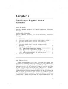
Note that αj* = 0 in (17a) and so is αj = 0 in (17b). Again, it is much better to calculate the bias term b by an averaging over all the free support vector data points. There are few learning parameters in constructing SV machines for regression. The three most relevant are the insensitivity zone ε, the penalty parameter C (that determines the trade-off between the training error and VC dimension of the model), and the shape parameters of the kernel function (variances of a Gaussian kernel, order of the polynomial, or the shape parameters of the inverse multiquadrics kernel function). All three parameters’ sets should be selected by the user. To this end, the most popular method is a crossvalidation. Unlike in a classification, for not too noisy data (primarily without huge outliers), the penalty parameter C could be set to infinity and the modeling can be controlled by changing the insensitivity zone ε and shape parameters only. However, in the case of high noise, or in the presence of outliers, it is highly recommended to use penalty parameter C which helps in ignoring the outlying points and may improve the generalization capacity of the final model significantly. The example below shows how an increase in an insensitivity zone ε has smoothing effects on modeling highly noise polluted data. Increase in ε means a reduction in requirements on the accuracy of approximation. It decreases the number of SVs leading to higher data compression too. Example: Construct an SV machine for modeling 31 data pairs. The underlying function (unknown to the SVM) is f(x) = x2sin(x)) and it is corrupted by 25% of normally distrib-

uted noise with a zero mean. Analyze the influence of an insensitivity zone ε (ε = 1, and ε = 0.75) on modeling quality and on a compression of data, meaning on the number of SVs. Two solutions are shown in Fig. 2 below. The approximation function (a thick solid red line) is created by 9 and 18 weighted Gaussian basis functions for ε = 1 and ε = 0.75 respectively. These supporting Gaussian functions are not shown in the figure. However, the way how the learning algorithm selects SVs is an interesting property of support vector machines and in Fig 3 we also present the supporting Gaussians. Note that the selected Gaussians lie in the dynamic area of the function in Fig 3. Here, these areas are close to both the left hand and the right hand boundary. In the middle, the original function is pretty flat and there is no need to cover this part by supporting Gaussians. The learning algorithm realizes this fact and simply, it does not select any training data point in this area as a support vector. Note also that the Gaussians are not weighted in Fig 3, and they all have the peak value of 1. The standard deviation of Gaussians is chosen

10

Vojislav Kecman

in order to see Gaussian supporting functions better. Here, in Fig 3, σ = 0.6. Such a choice is due the fact that for the larger σ values the basis functions are rather flat and the supporting functions are covering the whole domain as the broad umbrellas. For very big variances one can’t distinguish them visually. Hence, one can’t see the true, bell shaped, basis functions for the large variances. One-dimensional support vector regression by Gaussian kernel functions

5 4

One-dimensional support vector regression by Gaussian kernel functions

6

y

y

4

3 2

2

1 0

0 -1

-2 -2 -3

-4

-4

x

x

-5

-6 -3

-2

0

-1

1

2

3

-3

-2

-1

0

1

2

3

Figure 2 The influence of an insensitivity zone ε on the model performance. A nonlinear SVM creates a regression function f with Gaussian kernels and models a highly polluted (25% noise) function x2sin(x) (dotted). 31 training data points (plus signs) are used. Left: ε = 1; 9 SVs are chosen (encircled plus signs). Right: ε = 0.75; the 18 chosen SVs produced a better approximation to noisy data and, consequently, there is the tendency of overfitting. y

1-dimensional SVMs regression by Gaussian functions - the selected supporting Gaussian functions are also shown

4 3 2 1 0 -1 -2 -3 -4 x -5

-3

-2

-1

0

1

2

3

Figure 3 Regression function f created as the sum of 8 weighted Gaussian kernels. A standard deviation of Gaussian bells σ = 0.6. Original function (dashed thick line) is x2sin(x) and it is corrupted by . 25% noise. 31 training data points are shown as plus signs. Data points selected as the SVs are encircled. The 8 selected supporting Gaussian functions are centered at these data points.

2 Active Set Method for Solving QP Based SVMs’ Learning4 In both the classification SVMs and the regression ones the learning problem boils down to solving QP problem subject to the so-called ‘box’-constraints and to the equality constraint in the case that a model with a bias term b is used. The size of the QP’s Hessian matrix H and its density (the sparser the better for solving the QP problem) define the feasibility of the solution. Unfortunately, in SVMs training, Hessian H is always (extremely) dense (meaning ill-conditioned) and it scales with the number of data N. Thus, the SV training works almost perfectly for not too large training data set. However, when the number of data points is large (say N > 2,000) the QP problem becomes extremely difficult to solve with standard QP solvers and methods. For example, a classification training set of 50,000 examples amounts to a Hessian matrix H with 2.5*109 (2.5 billion) elements. Using an 8byte floating-point representation we need 20,000 Megabytes = 20 Gigabytes of memory (Osuna et al, 1997). This cannot be easily fit into memory of present standard computers, and this is the single basic disadvantage of the SVM method. There are four basic approaches that resolve the QP for large data sets. Vapnik in (Vapnik, 1995) proposed the chunking method that is the decomposition approach falling into the class of active set approaches. Another decomposition algorithm is suggested in (Osuna et al, 1997). The sequential minimal optimization (SMO) algorithm (Platt, 1997) is of different character and it seems to be very popular in SVM learning. The most recent Huang and Kecman’s Iterative Single Data Algorithm (ISDA) software seems to be the fastest one and very efficient for huge data sets (Kecman, Huang and Vogt, 2005; Huang, Kecman and Kopriva, 2006). SMO and ISDA belong to the so-called working set algorithms. A systematic exposition of these various techniques is not given here, as all four would require a lot of space. Vogt and Kecman in (Vogt & Kecman 2004, 2005) present and discuss the application of an active set algorithm in solving small to medium sized QP problems. The method also works for large data sets and very ill-conditioned matrix H setting, providing that the number of SVs is not too high a percentage of the training data used. For such data sets, and when the high precision is required, the active set approach in solving QP problems is superior to other approaches (notably the interior point methods, and working set ones SMO and ISDA algorithms). (Vogt and Kecman, 2005) can be downloaded from http://www.support-vector.ws). Active-set algorithm’s suitability is due to the fact that they need O(Nf 2 + N) memory where Nf is the number of free (unbounded, |α|i < C) SVs. Nf is typically much smaller than the number of the data N, and it dominates the memory consumption for large data sets due to its quadratic dependence. The basics of active set method and its comparisons with the SMO based algorithms are given in the references above where the detailed derivation of the active set is pre4

This part on active set method for solving SVMs QP problem can also be skipped. It talks about the motives and inspirations that led to developing an AS-LS algorithm which will be introduced in section 3, page 15. However, there is a deeper connection between the active set solution of the SVMs QP problem, and AS-LS which can be found at the bottom of page 34.

12

Vojislav Kecman

sented for both classification and regression problems without the bias term b and with it. In addition, all the details of the implementation by using Cholesky decomposition are presented in 2005 reference. Below, just the basic idea of an active set algorithm for SVMs is presented and later transformed into solving regression tasks by active set least squares method. Active set algorithms are the classical solvers for QP problems. They are known to be robust, but they require more memory than working set algorithms. The first active sets algorithms utilized for training the SVMs in an almost identical way for classification and regression are derived in (Vogt & Kecman 2004). The general idea is to find the active set A, i.e., those inequality constraints that are fulfilled with equality. If the set of active support vectors A is known, the Karush-Kuhn-Tucker (KKT) conditions reduce to solving simple system of linear equations which leads to the solution of the QP problem. Thus, active set algorithm is an iterative procedure where in each iteration step a single SV, the worst KKT violator, is added to the active set. In the beginning of computation A is unknown and it must be constructed iteratively by adding and removing constraints and testing if the solution remains feasible. The construction of A starts with an initial active set A0 containing the indices of the bounded variables (lying on the boundary of the feasible region) whereas those in F0 = {1, . . . , N}\ A0 are free (lying in the interior of the feasible region). Then the following steps are performed repeatedly for k = 1, 2, …: S1. Solve the KKT system for all variables in Fk. S2. If the solution is feasible, find the variable in Ak that violates the KKT conditions most, move it to Fk, then go to S1. S3. Otherwise find an intermediate value between old and new solution lying on the border of the feasible region, move one bounded variable from Fk to Ak, then go to S1. The intermediate solution in step S3 is computed by affine scaling as a k = η a k + (1 − η )a k −1 with maximal η∈ [0, 1] , where a k is the solution of the linear system in step S1, i.e., the new iterate a k lies on the connecting line of a k −1 and a k . The optimum is found if during step S2 no violating variable is left in Ak. See in (Vogt and Kecman, 2005) for all the details. Active set learning algorithm for the regression problems is to solve the following system of equations in each S1 step, H k a k = ck

(18)

where

aik = α ik − α i*k k ij

h = K ij

for i ∈ F k ∪ F *k

(19)

2 Active Set Method for Solving QP Based SVMs’ Learning

cik = yi −

∑

a kj K ij +

j∈ ACk ∪ AC* k

13

−ε for i ∈ F k

ε for i ∈ F *k

Note that in the active set method one uses variables ai = α i − α i* and just the size of the matrix H is a half of the one in classic SVMs regression setting. Sets ACk and AC*k contain all the indices of the bounded SVs, meaning the ones for which α ik = C , α i*k = C . Also note that in the first step (k = 1), the worst violating data is chosen, and then k increases to 2, 3, 4, …., and so on. Thus, in each step there is one more equation to solve. Step S2 of the algorithm calculates

λik = ε + Eik λi*k = ε − Eik

for i ∈ A0 k ∪ A0*k

(20a)

for i ∈ AC k ∪ AC *k

(20b)

and

µik = −ε − Eik µi*k = −ε + Eik

where Ei = f (xi ) − yi denotes the prediction error. The multipliers λi and µi are checked for positiveness with precision τ, and the variable with the most negative multiplier is transferred to Fk or F*k. The algorithm above is valid for positive definite kernels when the model does not have bias term. In the case of bias term there is slightly change of equation (18) only. Graph in Fig 4 below shows the active set steps more clearly. An implementation is as follows: The most memory required and the biggest CPU time consuming part is solving system of equations (18). Since all the algorithms assume positive definite kernel functions, the kernel matrix H has a Cholesky decomposition H = RTR, where R is an upper triangular matrix. For a fixed bias term, the solution of the linear system in step S1 is then found by simple back-substitution. For variable bias term, the blockalgorithm as described in (Vogt and Kecman, 2005) is used. The use of Cholesky decomposition speeds up the calculation a lot. There are many details to care about during the implementation while adding to and removing from the variables of an existing Cholesky decomposition. Also, a clever strategy should be used for implementing shrinking heuristics and for cashing kernel values. (See the reference above). Before introducing active set least squares algorithm for regression we will point out basic findings about the active set method for training SVMs. Experimental results show that active-set methods are advantageous • • • • •

for ‘medium’ sized data sets, when the number of support vectors is small, when the fraction of bounded variables is small, when high precision is needed, when the problem is ill-conditioned.

14

Vojislav Kecman Initialization

Solve linear system on F

Solution feasible

no

Reduction step Move blocking variables to A

yes

affine scaling

Find worst KKT violator in A

a2 a Move violators to F

yes

Violator found no

k

a2, a2 ≥ 0 a = η a k + (1 − η )a k −1 k

a k −1

a1

STOP

Figure 4 Flow chart of an active-set algorithm and affine scaling of the non-feasible solution (M. Vogt’s graph, 2006)

In the rest of the report, the active set least squares algorithm will be introduced by using the same approach in selecting worse violating data point as the active set method for training the SVMs. The worse violating data point is the one where there is the biggest deviation of the measured target values from the actual approximating function in the k-th iterative step. However, weight vector at the step k + 1 wk + 1 will be calculated differently. Next, the Householder reflections based QR factorization method in an updating form will be presented ensuring accurate and fast method for solving least squares problems arising within the AS-LS. This is the tool proposed here for calculating wk + 1. Then, the AS-LS algorithm for constrained values of the weights will be developed and finally, the comparisons with the SVMs on two standard regression benchmark problems will be shown. Note that the proposed AS-LS algorithm is relaxing many requirements present in SVMs. First, the basis functions don’t have to be strictly positive definite kernels. Any basis functions ensuring full rank of matrix H will do. Second, basis function don’t have to be associated with the measured training inputs. Third, and this may eventually be the strongest point in the future, more than a single basis function can be associated with each training data point (e.g., several Gaussian hyperbells with different widths may be placed at a single data points). The last opportunity will only cause slower learning (with a decrease in a speed being proportional to the number of basis functions used at a single data points) offering at the same time possibly huge improvements in modeling performance (higher accuracy, less SVs, higher accuracy).


15


The basic feature of the active set method for SVMs is that in each iteration step k, the values of dual variables α ik , α i*k are solutions of a linear system for k support vector variables by using only the selected k variables. In other words, if in some iteration step the training data (regressors, support vectors) m, n, o, p and q are selected the matrix H will be a square (5, 5) matrix formed of columns and rows m, n, o, p and q, and the current approximating function fa(x) will be created only by data points m, n, o, p and q. The approximator fa(x) accommodates desired values ym, n, o, p, q on the ε-tube. The rest of training data does not contribute to the forming of current approximating function fa(x) at all. Thus, in-between the data points m, n, o, p and q the function fa(x) may behave (and it usually does) as ‘wild’ and as ‘hairy’ as needed to suit only the five outputs yi (i = m, n, o, p, q) on the ε-tube. The unselected data points (non-regressing data, i.e., non-SVs at the step k) do not have any (primarily smoothing) influence on fa(x). Thus, at the end of a learning, the final approximating function fa(x) will be the one created without any influence of the great portion of the training data points i.e., fa(x) is ignoring them as long as they are fitted within the εtube in the case of the hard regression. As for the soft regression, some data points will be allowed to be left out of the tube and their corresponding dual variables α i and α i* will be bounded at the value of the penalty parameter C. The ‘wild’ behavior of fa(x) is illustrated by an approximation of a ‘dynamic’ 1dimensional function in Figs 5 where the first few iterations and two final ones are shown. Left column shows a progression of approximations by an active set SVMs (thick solid red line with the ε-tube shown, ε = 0.75), while the right one shows the approximations obtained by the active set least squares method (blue thick curve). In all simulations data was spoiled by 10% Gaussian noise having zero mean. The width of Gaussians was 9 times an average distance between the data points. Note that the final AS-LS model is sparser (29 SVs only) than a classic SVM’s one (45 SVs). Note also that in the case of an active set SVM (left column graphs) the sum of errors squares over all the training data generally decreases but in a wild, non-smooth, manner. Therefore, it can’t be used as reliable stopping criterion. This is not the case with the ASLS (right column graphs) where the sum of error squares continuously decreases by an increase in a number of selected SVs (basis functions, hidden layer neurons, regressors). Hence, in an addition to the fitting of all the training data inside the ε-tube sum of errors squares over all the training data can, and it will, be used as a stopping criterion for the AS-LS algorithm.

16

Vojislav Kecman

SVMs Approximation by 1 Support Vectors

Solution obtained by 1 RBF Support Vectors

35

35

30

30

25

25

20

20

15

15

10

10

5

5

0

0

-5

-5

-10

-10

0

2

4

6

8

10

12

0

SVMs Approximation by 2 Support Vectors 35

30

30

25

25

20

20

15

15

10

10

5

5

0

0

-5

-5

-10

-10

2

4

6

8

4

6

8

10

12


35

0

2

10

12

0

2

SVMs Approximation by 3 Support Vectors

4

6

8

10

12


35

35

30

30

25

25

20

20

15

15

10

10

5

5

0

0

-5

-5

-10

-10

0

2

4

6

8

10

12

0

2

4

6

8

10

12

Figure 5 Progression of approximations: left column - by active set SVMs (red solid curve with the

ε-tube shown), and right column - by active set least squares method (blue solid curve). Green stars * are 100 training data, blue dashed curve is true function, and current SVs are encircled data points. Figure continues on the next page.




35

30

30

25

25

20

20

15

15

10

10

5

5

0

0

-5

-5

-10

-10

0

2

4

6

8

10

0

12

2


30

30

25

25

20

20

15

15

10

10

5

5

0

0

-5

-5

-10

-10

2

4

6

8

10

4

6

8

10

12


35

0

17

12

0

2

4

6

8

10

12



35 30

30

25

25

20

20

15

15

10

10

5

5

0

0

-5

-5

-10

-10

0

2

4

6

8

10

12

0

2

4

6

8

10

12

Figure 5 (continued) Progression of approximations: left column - by active set SVMs (red solid

curve with the ε-tube shown), and right column - by active set least squares method (blue solid curve). Green stars * are 100 training data, blue dashed curve is true function, and current SVs are encircled data points. Figure continues on the next page.

18

Vojislav Kecman Solution obtained by 21 RBF Support Vectors


35

30

30

25

25

20

20

15

15

10

10

5

5

0

0

-5

-5 -10

-10

0

2

4

6

8

10

0

12


30

30

25

25

20

20

15

15

10

10

5

5

0

0

-5

-5

-10

-10

2

4

6

8

10

4

6

8

10

12


35

0

2

12

0

2

4

6

8

10

12

Figure 5 (continued) Progression of approximations: left column - by active set SVMs (red solid

curve with the ε-tube shown), and right column - by active set least squares method (blue solid curve). Green stars * are 100 training data, blue dashed curve is true function, and current SVs are encircled data points.

The non-smooth behavior of the approximating functions shown in the left columns of the graphs in Fig 5 led naturally to the idea of changing the active set method for SVMs so that instead of solving the system of k linear equations in k unknowns (18) originating from k selected regressors (i.e., SVs), one solves an overdetermined system of N equations in k unknowns in the least squares sense as given below Hk wk ≅ y

(21)

where Hk is an (N, k) matrix and y is the complete desired (N, 1) vector. Thus, if in step k the training data (regressors, support vectors) m, n, o, p and q are selected, the matrix Hk will be a rectangular (N, 5) matrix formed of columns obtained by kernels m, n, o, p and q but now, the kernels (basis functions) will be calculated for all the N available training data points. After solving (21) for wk, the approximating function fa(x) at each step k equals fa(x)k = Hkwk Having fa(x)k one finds the worst violating data point xwv from

(22)


(

)

Arg max abs y − f a (x) k .

19

(23)

x wv

xwv is then added to the set of supporting vectors F for solving the system H k +1w k +1 = y in the next iteration step. Thus, in the iteration step k + 1 matrix Hk+1 is an (N, 6) matrix, and 6 weights for 6 basis functions have to be found. This algorithm is called the active set least squares (AS-LS) method. AS-LS works with or without bias term b. In the case that one wants to use the bias term b the first system to be solved in a first step (k = 1) is H1 w1 = 1w1 ≅ y

(24)

where 1 = [1 1 1 … 1]T i.e., it is an (N, 1) vector of ones. It is obvious that the first approximating function fa(x)1 will model the constant mean value of the data.

3.1 Implementation of the Active Set Least Squares Algorithm

One of the basic requirements of any new machine learning (data mining) algorithm is to be able to handle huge amount of data and to do the calculation as fast as possible. This naturally concerns the AS-LS algorithm which is aimed at ‘medium’ sized data and the ‘medium’ is defined as the size at which the matrix Hfinal can still be stored in the memory of the computer, where the matrix Hfinal is an (N, NSV) size matrix. Actually, the storing can also take place at hard drive and then the definition ‘medium’ just increases. However, reaching hard drive at each iteration step may be time consuming, and hard drive damaging too, so we stick to the previous definition. Thus, the task to solve now is to develop fast updating algorithm for solving an increasing in the size series of least squares problems. There are many algorithms that can be used for solving least squares problems (forming normal system of equations, application of the pseudo-inversion, using ShermanMorrison-Woodbury formula, performing LU decomposition, doing an SVD factorization and the list goes on. For an extensive analysis of the properties of various LS algorithms the reader is referred to (Mrosek, 2006). However, for many reasons (foremost due to its impeccable numerical properties) the most promising approach is to use the QR decomposition as given below R k  R k  Q k H k =  k  , or H k = Q kT  k  0  0 

in an iterative updating fashion.

20

Vojislav Kecman

3.1.1 Basics of Orthogonal Transformation

Decomposing the matrix H (N, k) into an (N, N) orthogonal matrix Q (QQT = QTQ = I) and an upper triangular matrix R (N, k) avoids all the numerical difficulties while using the normal system of equations. Thus, the QR factorization of a matrix is one of the most powerful factorization and the one realized by Householder reflections (HRs) is numerically impeccable method. This is why the MATLAB’s backslash operator uses the Householder reflections. (The other three methods for the QR decomposition are the Gram-Schmidt orthogonalization, modified Gram-Schmidt orthogonalization and an application of Givens rotations). In addition to its great numerical properties, the QR algorithm based on the HRs can be easily transformed into an efficient iterative updating routine which is of particular interest for AS-LS approach in regression. In solving LS problems, a nice property of the orthogonal matrix that it preserves the Euclidean norm of the vector v is used. Namely, the following is valid, Qv

2 2

2

T

= ( Qv ) ( Qv ) = vT QT Qv = vT v = v 2 ,

(25)

and this will be exploited in sequel. Additionally, there is a benefit of having the upper triangular matrix R due to its usability in solving an overdetermined linear system of equations by a back-substitution. Namely, in solving  v1  R   0  w ≅ v  ,    2

(26)

it turns out that the error (residual) is 2

2

2

e 2 = v1 − Rw 2 + v 2 2 ,

(27)

and, because the regular square system of equations Rw = v1 can be exactly solved, the 2

minimal squared error equals v 2 2 . Thus, in each iteration step, the QR factorization

factorizes the (N, k) matrix Hk into the product of an (N, N) orthogonal matrix QT and the matrix [RT 0T]T where R is an (k, k) upper triangular matrix as follows R k  H k = Q kT   , 0 

(28)

Thus, the overdetermined LS problem (21) H k w k ≅ y is, after multiplying by Q, transformed into the triangular LS task as shown below (indexing by k is avoided for the sake of notation’s simplicity ) v  R  QHw =   w ≅ Qy =  1  . 0    v2 

(29)

The last expression has the same solution as Hw ≅ y because multiplying both sides of a least-squares equation by an orthogonal matrix Q doesn’t change the solution. This follows from the fact in (25) which shows that the orthogonal transformation preserves the Euclidean norm. Namely, the lines shown below


2

e 2 = y − Hw

2 2

R  = y −Q  w 0

2

T

2

R  = Qy −   w 0

21

2 2

= v1 − Rw 2 + v 2

2 2

2

= v 2 2 , (30)

2

prove that the norm of the solution error doesn’t change after application of QR transformation.

3.1.2 An Iterative Update of the QR Decomposition by Householder Reflection

There are many ways how one can apply QR factorization while solving LS tasks. In (Mrosek, 2006) the following MATLAB’s implementation have been investigated - standard QR factorization, transpose QR factorization, economy size QR factorization, column insert QR factorization, column append QR factorization and QR factorization without computing Q matrix (limited to sparse matrices). The column append QR factorization is not a standard MATLAB routine. It is an Mrosek’s MATLAB implementation of the algorithms from Craig Lucas’ PhD thesis (Lucas, 2004). (There are few more routines based on Givens rotations presented in the thesis). As shown in (Mrosek, 2006) the MATLAB’s insert column and append one are the fastest routines for solving LS problems. In this section we introduce an even faster QR implementation particularly suited for an iterative (appending columns) procedure as required in AS-LS, which was used for the experiments here. This is an iterative method for solving a series of equations (21) based upon the Householder reflections as introduced in (Moler, 2004) and implemented here and in (Mrosek, 2006). This novel implementation of the Householder algorithm avoids the calculation of matrix Q at any stage of the solution, and it is capable of solving the linear least squares problem arising from the AS-LS algorithm faster than all the other alternative algorithms for solving LS problems. To compute a QR factorization of matrix H, HRs are performed in order to annihilate subdiagonal entries of each successive column of H. This is done by a sequence of transformations applied to the columns h of the matrix H to produce the matrix R, where in each step i a transformation matrix Ti is formed as follows Ti = I − 2

vi viT . v iT v i

(31)

In order to transform the vector h, the vector v used in (31) is formed as shown below 2

v = h − α e, α = ± h 2 ,

(32)

and the sign of α is chosen to avoid the cancellation of i-th entry of the transformed column h. Suppose we want to apply an HR to the vector h = [-1 2 3]T. First we form vector

22

Vojislav Kecman

 −1 1   −1 α   −4.7417  v =  2  − α  0 =  2  −  0  , α = h = 3.7417, v =  2  ,  3   0  3   0   3  where the sign for α is chosen positive because v1 is a negative number. The matrix T is

T = I−2

-0.2673 0.5345 0.8018  3.7417  vvT   ⇒ Th =  0  = 0.5345 0.7745 -0.3382    vT v   0.8018 -0.3382 0.4927   0 

If one wants to transform solving of the LS problem Hw = y into solving the system of equations using the upper triangular matrix R, the matrix H should be transformed by applying a sequence of HRs to H such that QH = R or H = QTR. For a matrix H given as 1 1  1 H= 1 1  1 this is performed by starting T 2

h1 = [1 1 1 1 1 1]

2

2 3 3 3  2 3  1 2 1 2  1 2 

with the first column (note that the norm

= 2.4495 ), creating the vector v1, making the reflection ma-

trix T1,

1  −2.4495 3.4495 -0.4082 -0.4082 -0.4082 1  0   1  -0.4082 0.8816 -0.1184       1  0   1  -0.4082 -0.1184 0.8816 v1 =   −  =  , T1 =  1  0   1  -0.4082 -0.1184 -0.1184 1  0   1  -0.4082 -0.1184 -0.1184       -0.4082 -0.1184 -0.1184 1  0   1  and multiplying H by T from left as below

-2.4495  0.0000   0.0000 T1H =   0.0000  0.0000   0.0000

-4.0825 -6.1237  1.2367 0.3551  0.2367 0.3551  . -0.7633 -0.6449  -0.7633 -0.6449   -0.7633 -0.6449 

-0.4082 -0.4082 -0.4082  -0.1184 -0.1184 -0.1184  -0.1184 -0.1184 -0.1184   0.8816 -0.1184 -0.1184  -0.1184 0.8816 -0.1184   -0.1184 -0.1184 0.8816 


23

Next, the transformation matrix T2 is calculated by first forming vector v2 from the matrix T2H above as follows,

0    1.2367     0.2367     -0.7633  -0.7633    -0.7633

2

2

 0   0   0  1.2367   −1.8257  3.0624        0.2367   0  0.2367  = 1.8257, v 2 =  − = , -0.7633  0  -0.7633 -0.7633  0  -0.7633       -0.7633  0  -0.7633

0 0 0 0 0 0 1   0 -0.6774 -0.1296 0.4181 0.4181 0.4181     0 -0.1296 0.9900 0.0323 0.0323 0.0323  T2 =    0 0.4181 0.0323 0.8958 -0.1042 -0.1042   0 0.4181 0.0323 -0.1042 0.8958 -0.1042     0 0.4181 0.0323 -0.1042 -0.1042 0.8958  Notice the way how the vector v2 is formed from the 2nd column of a matrix T1H, above (v2(1) was set to 0) and follow the same way in forming the vector v3 from the 3rd column of the matrix T2T1H below -2.4495 0.0000  0.0000 T2 T1H =  0.0000 0.0000  0.0000

-4.0825 -6.1237  -1.8257 -1.0954  0.0000 0.2429  . 0.0000 -0.2834  0.0000 -0.2834   0.0000 -0.2834 

Now we’ll use the slightly changed 3rd column of T2T1H in forming the vector v3 namely, this one [0 0 0.2429 -0.2834 -0.2834 -0.2834]T is used in calculation of v3 below

 0   0    0.2429    -0.2834 -0.2834   -0.2834

2

2

 0   0   0   0   0   0        0.2429   −0.5477  0.7907  = 0.5477, v 3 =  − = , -0.2834   0  -0.2834 -0.2834   0  -0.2834       -0.2834   0  -0.2834

24

Vojislav Kecman

    T3 =     

1.0000 0 0 0 1.0000 0 0 0 -0.4435 0 0 0.5175 0 0 0.5175 0 0 0.5175

0 0 0.5175 0.8145 -0.1855 -0.1855

0 0   0 0  0.5175 0.5175   -0.1855 -0.1855 0.8145 -0.1855  -0.1855 0.8145

The sequence of Householder transformations produced the following QR factorization of matrix H R  T3 T2 T1H =   0 Note two interesting facts; first a product of transformation matrices Ti equals the orthogonal matrix Q,     Q = T3 T2 T1 =     

-0.4082 -0.1826 -0.5477 -0.4082 -0.4082 -0.4082

-0.4082 -0.7303 0.5477 0.0000 0.0000 0.0000

-0.4082 -0.1826 -0.5477 0.4082 0.4082 0.4082

-0.4082 0.3651 0.1826 0.6667 -0.3333 -0.3333

-0.4082 0.3651 0.1826 -0.3333 0.6667 -0.3333

-0.4082  0.3651  0.1826   -0.3333  -0.3333   0.6667 

and second, the explicit form of Q was not needed for computing the triangular matrix R. This fact will be used in implementing iterative updating algorithm for AS-LS increasing in this way the speed of computation as well as reducing the memory space for not saving the matrix Q at all. The algorithm to implement starts with the first LS equation to solve H1w1 = h wv1w1 ≅ y

(33)

After finding the first transformation matrix T1 HR is performed and one gets

 y1   r1  y  0  2   1 1 T1h wv1w =  0  w ≅ T1  y3          yN   0 

(34)

Having the first weight w1 calculated from (34) the approximating function fa(x)1 = h1w1 is computed and the worst violator is found. Now, the column vector corresponding to the


25

worst violator is appended to the previous matrix H1, new matrix T2 is to be found and the process repeats itself until some stopping criterion is met. The stopping criterion is either fitting all the data within the prescribed ε-tube, or the updating and increasing the size (number of basis functions, regressors, SVs) of the model goes as long as the sum of error squares decreases. It is easy to show that the sum of error squares for an AS-LS algorithm can’t increase at any point. This is contrary to the behavior of an error function in SVMs’ learning when the change of cost function can be fairly wild. Note also that the proposed AS-LS algorithm does not delete already selected support vectors from the active set. Once SVs is chosen, means a selection ‘for life’. Also note that adding new regressors typically deteriorates the condition number of matrix H, and if the ‘fitting within the tube’ is not met, the training goes until the condition of the matrix Hk is so bad that the error starts increasing due to the loss of the rank of some sub-matrices within the routine. The whole art and science of solving AS-LS learning problems focuses now on a sophisticated code for implementing an iterative sequence of HRs presented earlier while avoiding calculation of a Q matrix and by saving as much of computer memory as possible, having in mind that the algorithm should be able to cope with huge number of training data. Within this report and jointly with (Mrosek, 2006) two codes for an orthogonalization of the LS problem arising in AS-LS method given in appendix have been developed showing the better performance (great accuracy, faster algorithm and lower requirements on a memory) than all the other QR factorization implementations. These two codes are hhcolappend.m and backsubs.m. Note that in each iteration step both routines are called for a calculation of the weight vector w, followed by finding the approximation function fa, picking up the worst violator xwv, adding it to the set of selected basis functions, and running the new iteration step. (How such an updating works on a 1-dimensional problem in approximating a decreasing sinus function is shown in the Appendix). The final LS problem to solve at the point of stopping in the step K is the one with (N, K) matrix H, and the (K, 1) weight vector w obtained from the least squares solution of the equation Hw = y. As it can readily be seen, when the number of data goes into thousands one better hopes the number of supporting vectors K be just a small fraction of the training data set. Luckily, at many instances this is often the case. However, if it is not that way one should either take into account slow learning process or one must switch to the working set kinds of algorithms for training SVMs (ISDA or SMO for example). The AS-LS has shown very good results on some renown benchmark, and some tough although toy in size, problems. This will be shown shortly. Now, however, we’ll extend the AS-LS learning algorithm to the one with a weight constraints.

26

Vojislav Kecman

3.2 An Active Set Least Squares with Weights Constraints – Bounded LS Problem As it is very well known, solving LS problems when the matrix H is not well conditioned (which is often the case in machine learning) results in huge values of the weight vector. This is a consequence of the fact that with an increase of the conditional number the value of the determinant of the matrix H approaches zero, and it is this value which is in the denominator while calculating the vector w whenever one uses matrix inversions. Here, while applying HRs one doesn’t use the inverse at any point but the effects of bad conditioning are present and they lead to high weights’ values through the very low values of the matrix R too. For badly conditioned matrices the upper triangular matrix R is closing to the singular matrix. At the same time, constraining the weights used to be and still is a standard and traditional method in avoiding data overfitting and basically bad performance of the model associated with it. This idea has been lifted particularly high in the learning algorithms for SVMs where (initially the only, and today) the important part of the cost function is a norm of the weight vector w which must be as small as possible. Constraining the weights values is both a right and good step and it is one of the basic foundations of the statistical learning theory (Vapnik, 1995, 1998). Therefore, after the experiments with the AS-LS algorithm have often resulted with the huge weights’ values, the natural extension of the AS-LS is to enable learning with limiting the weights. A novel AS-LS algorithm with weights constraints will be presented in this section. Before presenting the algorithms developed and used within this report it has to be mentioned that few more routines and approaches have been tested for solving the bounded least squares (BLS) problem (35) posed below. They have been performing fine on toy problems but all of them failed on a tougher benchmark problem (e.g., on the dynamic problem of a Mackey-Glass time series prediction). The first attempt was exploiting the MATLAB’s lsqlin routine. In addition, the sparse least squares Matlab toolboxes (SBLS and SBLS2) developed within the PhD thesis presented in (Adler, 2000) have also been used. None of the algorithms has shown good performance beyond the ‘toy’ 1-D problems. As for SBLS and SBLS2 routines developed for sparse problems, it was hard to believe that they may perform well on problems involving extremely dense matrices. This is why another, more efficient, approach has been taken for solving the constrained AS-LS task below. In section 4 it is shown that such an approach for the bounded AS-LS algorithm competes favorably with the SVMs algorithm. The Active Set Bounded Least Squares (AS-BLS) problem to solve now is - in each iteration step k find wk of the LS problem Hk wk ≅ y ,

(35a)

−C ≤ wi ≤ C , i = 1, k .

(35b)

such that


27

This is resolved by applying the series of algorithms introduced in (Lawson, Hanson, 1995) as follows. First, by an introduction of a (2k, k) matrix K = [I -I]T and a (2k, 1) vector c = [-C -C . . . -C]T problem (35) is transformed into the least squares problem with linear inequality constraints (LSI) which is posed as - minimize

Hw − y

w

,

(36a)

subject to

Kw ≥ c .

(36b)

The LSI problem is transformed into the least distance programming (LDP) task which, finally, uses the non-negative least squares (NNLS) algorithm as the solving tool. The mentioned sequence of routines is given in Fig. 6 graphically.

H, y , K, c

KKR, c-KKR*y1 LSI

w

E = [K ’; c’], f LDP

x=-r/rnn , r = Eu - f

u NNLS

u

Figure 6 The sequence of algorithms for solving Active Set Bounded Least Squares problems

Here, in creating the final efficient sequence of three algorithms the Rasmus Bro’s implementations of LSI and LDP (Rasmus, 2006) were combined with Uriel Roque’s (Roque, 2006) block pivoting algorithm from (Portugal et al, 1994) which may update more than one element at the same time and is more robust and faster than other NNLS algorithms tried within the AS-BLS loop in Fig 6. Here, the Roque’s blocknnls.m was slightly adapted in order to robustly handle dense badly conditioned matrices appearing in AS-BLS regression algorithm. Basically, the breaking line of the code (when certain sub-matrices involved in solving NNLS lose their rank) has been introduced. This simple addition closed the loop in Fig 6 and made the whole AS-BLS a robust algorithm. The most CPU time consuming part of the algorithm is solving the NNLS problem. This is particularly critical when the data sets is big (several thousands of training data) and the character of the problem is such that good model needs a lot of supporting data points (regressors, SVs, basis functions) in creating final approximation function. In the experimental part of the report (performed in MATLAB) many algorithms for solving NNLS have been tried and most of them failed on Mackey-Glass time series prediction due to conditioning of underlying matrices. (However, all of them perform nicely for smaller and well conditioned problems). Conditioning is related to the parameters of the kernels used. It basically increases with higher overlapping of Gaussian radial basis kernels (‘big’ width parameter σ of Gaussian ‘hyper-bells’) as well as with the increase of the order of the poly-

28

Vojislav Kecman

nomial kernels. The simulations have been executed by using MATLAB’s lsqnonneg.m as well as Rasmus’ fnnls.m, and Roque’s three different solvers for NNLS problem – Predictor-Corrector solver pcnnls.m, Active Set solver activeset.m, and Newton’s solver newton.m. Note that solving regression tasks in high dimensional spaces by kernels usually leads to extremely badly conditioning of matrices involved and this is why none of the routines performed well for various reason (one is aimed at squares matrices only, another one is prone to cycling of the algorithm, yet another one looses the rank of some sub-matrices, or some are slow and just leading to the seemingly never ending convergence etc). However, the Roque’s blocknnls.m was good enough and helped in proving the soundness of the AS-LS approach. With our tiny adaptation it has displayed very good performance on many problems as well as high modelling capacity. In the next section, it will be shown that both unconstrained AS-LS and bounded AS-BLS algorithms successfully compete with SVMs in solving complex benchmark problem of predicting very difficult to forecast dynamic Mackey-Glass time series.

29

4 Comparisons of SVMs and AS-LS Regression Predicting nonlinear dynamic (chaotic) system such as Mackey-Glass time series (Lapedes and Farber, 1987; Majetic, 1995, Mukherjee et al., 1997, Müller et al, 1998, Shah, 1998) is a very difficult task but such a series forms a good test to investigate the capability and performance of machine learning techniques. Here, we will compare performances of ASLS and AS-BLS algorithms with the results obtained by SVMs. There are many examples of chaotic systems in nature including - chemical reactions, turbulence phenomena in fluids, nonlinear vibrations, etc. Lapedes and Farber (1987) suggested and first used the Mackey-Glass time series as a good benchmark for neural networks learning algorithms since it has a simple definition but is still hard to predict. The Mackey-Glass equation is a non-linear differential delay equation (originally introduced as a model of a blood cell regulation) given as

ax ( t − τ ) dx = − bx(t ) dt 1 + x10 ( t − τ )

(37)

with a = 0.2, b = 0.1 and delay τ = 17. For 1,000 time steps the Mackey-Glass time series without the noise is shown in Fig 7. Mackey-Glass time series, no noise 1.4 1.3 1.2 1.1 1 0.9 0.8 0.7 0.6 0.5 0.4

0

100

200

300

400

500 Time

600

700

800

900

1000

Figure 7 The Mackey-Glass chaotic time series with a = 0.2, b = 0.1 and τ = 17 for 1,000 time steps

The objective of the forecast is to use known previous values in the time series to predict the value at some point in the future. In SVMs based prediction a mapping of the historical values is described as the function

b

g m bg b

g b

g

b

x t + P = f x t , x t − ∆ , x t − 2 ∆ ,..., x t − m∆

gr

(38)

where P is a prediction time in future, ∆ is a time delay and m is an integer defining the embedded dimension of the problem d = m + 1. Embedded dimension defines the number

30

Vojislav Kecman

of terms used in the input vector i.e., it defines the dimensionality of the input vector. Here, we make one step prediction. Therefore, P = 1, time delay ∆ = 6, and the so-called embedded dimension is 6, meaning m = 5. Thus, the model uses the training data pairs (xi, yi, i= 1, N ), where xi is a 6-dimensional vector of the inputs composed of a present value of the Mackey-Glass (M-G) series x(t) and 5 delayed ones, and the output is the next value of the M-G series x(t + 1). The function f is a subject of training for the SVMs model which maps the input data onto the output space x(t + 1). In all the simulations the initial condition was x(t = 0) = 0.9. Also, in order to minimize the effect of the initial conditions and to reach the steady-state the first 200 elements of the series are discarded. Here, the results are shown for three sizes of training data set. In all the experiments the length N of the training session and the test one was the same. The experiments have been performed for 250 pairs of the training and test data, 500 pairs and 1,000 ones. Thus, Fig 8 shows the setting of all the experiments where N stands for 250, 500 and 1,000.

Training data points 0

Test data points N 0

N

Figure 8 The setting of a training and testing phase for the Mackey-Glass time series. Three series of experiments have been done for N = 1,000, 500 and 250 data pairs

The data shown in Figs 7 and 8 are noiseless. The true training data used here are polluted by a Gaussian noise with zero mean and various variances as well as with the uniform noise. Test was always executed by using N noiseless data enabling in this way measuring the models’ ability to approximate the true time series. As it can be seen in the results tables, several noise levels have been used. The noise ratio (NR) is calculated as follows NR% =

2 σ noise 100%, , 2 σ data

(39)

where the variances are calculated as

σ2 =

2 1 N ( xi − x ) , ∑ i =1 N −1

(40)

4 Comparisons of the SVMs and AS-LS Regression

31

Four segments of the M-G series polluted with a noise of various levels are shown in Fig 9. The training data used were either one of the noisy samples shown.

Figure 9 Four segments of Mackey-Glass time series polluted with Gaussian noise of various levels

In the training phase, the training data pairs of the present and previous inputs at the step k and the next output ( x k , xk +1 ) = ([ xk xk − 6 xk −12 xk −18 xk − 24 xk − 30 ] , xk +1 ) are used in order to learn the mapping f(*). After the training, given some input vector x the model predicts next value just implementing the trained function as xˆk +1 = f

([ x

k

xk − 6 xk −12 xk −18 xk − 24 xk − 30 ]) ,

(41)

where the hat sign denotes the next estimated value of the time series. The test is, however, carried out in a dynamic fashion meaning by feeding back the estimated values xˆ and, in a test mode, the following mapping at each iteration step is performed xˆk +1 = f

([ xˆ

k

xˆk − 6 xˆk −12 xˆk −18 xˆk − 24 xˆk − 30 ]) .

(42)

In the test phase the performance of each selected model is estimated for three different scenarios as in (Müller et al, 1998). The error is calculated for the one step prediction, for the 100 steps prediction and in the dynamic prediction mode over the whole sequence of N data. The one step prediction is in fact static mapping where at no point estimated values xˆ is fed back and thus, it doesn’t influence future predictions. The prediction starts with the initial state at k = 31, and at each iteration step the known (measured) test data are used to predict the next value only. This is done for all known input vectors in a test set. It’s different for the 100 steps predicting scenario. Starting from the initial known input vector at k = 31, the 100 steps model feeds back the predicted outputs for the next 100 steps. Then, the known 132nd measured input vector composed of 6 known entries (not the estimated ones) is used and the next 100 steps are predicted, based upon the known initial states. A true dynamic scenario (model) starts from the initial state k = 31 and feeds back the predicted outputs for the all N - 31 test data.

32

Vojislav Kecman

The cost (error) functional E used is the root mean square error (RMSE) over all the predicted outputs for all three scenarios as follows E=

∑

N − 31 i =1

( xˆi − xi ) 2

N − 31

(43)

.

4.1 Performance of an Active Set Least Squares (AS-LS) - without Constraints

The experimental part is aimed at finding good AS-LS based machine learning model or the SVM one, by picking the right design parameters. Here, in all the simulation the Gaussian kernel is used and there are three design parameters for both AS-LS and SVMs. They are the penalty parameter C defining the maximal absolute weight value of the model, width of Gaussian basis functions σ and the size of the ε-tube defining desired closeness of the model to data points. (Note that picking C = ∞ and ε = 0 means that one wants to interpolate the data points, which is usually bad idea because one typically wants to filter the noise out). For both models a series of runs for various values of the design parameters have been performed and the results are shown in Tables 2 – 7. Table 2 1,000 data Mackey-Glass series – RMSE Comparisons AS – LS vs. SVMs Noise Normal

Uniform

NR %

1 step error AS-LS SVM

0 11 22.15 44.3 6.2 18.6

0.0001 0.0161 0.0219 0.0307 0.0115 0.0260

0.0003 0.0174 0.0241 0.0315 0.0111 0.0187

100 steps error AS-LS SVM

0.0014 0.0910 0.1398 0.1620 0.1090 0.1417

0.0043 0.1111 0.1342 0.1368 0.0816 0.1362

dynamic error AS-LS SVM

0.0186 0.1071 0.1148 0.2141 0.1183 0.1412

0.0951 0.1124 0.1146 0.1141 0.1205 0.1116

Table 3 500 data Mackey-Glass series – RMSE Comparisons AS – LS vs. SVMs Noise Normal

Uniform

NR %


0 11 22.15 44.3 6.2 18.6

0.0002 0.0214 0.0248 0.0400 0.0123 0.0208

0.0004 0.0213 0.0290 0.0407 0.0120 0.0183


0.0033 0.0887 0.1052 0.1297 0.0755 0.1254

0.0034 0.1114 0.1202 0.1210 0.0875 0.1149


0.0230 0.1148 0.1169 0.1257 0.1036 0.1258

0.0132 0.0750 0.1126 0.1116 0.1100 0.1152

Table 4 250 data Mackey-Glass series – RMSE Comparisons AS – LS vs. SVMs Noise Normal

Uniform

NR %


0 11 22.15 44.3 6.2 18.6

0.0007 0.0323 0.0307 0.0464 0.0179 0.0301

0.0009 0.0222 0.2860 0.0398 0.0176 0.0258


0.0104 0.0795 0.0946 0.1078 0.1077 0.1026

0.0296 0.0715 0.0928 0.0933 0.0969 0.0938


0.0090 0.0795 0.0851 0.0963 0.0786 0.0920

0.0311 0.0680 0.0804 0.0879 0.0707 0.0736


33

First three tables compare unconstrained (C = ∞) AS-LS models with the SVMs optimized over several penalty parameters C. Usually, and this is a typical LS method’s characteristics, this leads to high values of the output layer weights. From Tables 2 – 4 few conclusions can be drawn. First, there are three different models performances shown in the tables – static one (1-step prediction) and complete dynamic model, as well as one intermediate one (100 steps prediction). Thus, a model which is performing well on the 1step prediction doesn’t necessarily have to perform well on the 100-step prediction and/or on the dynamic model prediction. Second, both models perform similarly in terms of the RMSE on the test data. Third, unconstrained AS-LS has tiny advantages for more training data and Gaussian noise, while SVMs is a little better for smaller data sets and when the noise is uniformly distributed. However, such performances have been expected because SVMs basic claim is to be good on the tasks when the data sets are sparse and polluted by unspecified noise distribution. At the same time AS-LS has shown all the good characteristics of LS based solutions performing well when there are plenty of data polluted by normal noise distribution. The strength of SVMs comes also from a constraining of the weights vector’s norm and it may be interesting to see whether the bounding of the weights works for AS-LS approach. As, it is shown in tables 5 - 7 it works indeed, and constraining the weights in the AS-BLS routine has shown better performances working within the true SVMs environment – meaning for sparse uniformly polluted data points.

4.2 Performance of a Bounded Active Set Least Squares (AS-BLS) with Constraints

Table 5 1,000 data Mackey-Glass series – RMSE Comparisons AS – BLS & AS-LS vs. SVMs 1 step error Noise normal uniform

100 steps error

dynamic error

NR %

AS-BLS

AS-LS

SVM

AS-BLS

AS-LS

SVM

AS-BLS

AS-LS

SVM

22.15 44.3 6.2 18.6

0.0256 0.0345 0.0116 0.0220

0.0219 0.0307 0.0115 0.0260

0.0241 0.0315 0.0111 0.0187

0.1363 0.1376 0.1151 0.1376

0.1398 0.1620 0.1090 0.1417

0.1342 0.1368 0.0816 0.1362

0.1133 0.1141 0.1059 0.1157

0.1148 0.2141 0.1183 0.1412

0.1146 0.1141 0.1205 0.1116

Table 6 500 data Mackey-Glass series – RMSE Comparisons AS – BLS & AS-LS vs. SVMs 1 step error Noise normal uniform

100 steps error

dynamic error

NR %

AS-BLS

AS-LS

SVM

AS-BLS

AS-LS

SVM

AS BLS

AS-LS

SVM

22.15 44.3 6.2 18.6

0.0277 0.0386 0.0109 0.0170

0.0248 0.0400 0.0123 0.0208

0.0290 0.0407 0.0120 0.0183

0.0989 0.1220 0.0847 0.1224

0.1052 0.1297 0.0755 0.1254

0.1202 0.1210 0.0875 0.1149

0.1159 0.1267 0.1127 0.1139

0.1169 0.1257 0.1036 0.1258

0.1126 0.1116 0.1100 0.1152

Table 7 250 data Mackey-Glass series – RMSE Comparisons AS – BLS & AS-LS vs. SVMs 1 step error Noise normal uniform

100 steps error

dynamic error

NR %

AS-BLS

AS-LS

SVM

AS-BLS

AS-LS

SVM

AS BLS

AS-LS

SVM

11 22.15 44.3 6.2 18.6

0.0229 0.0312 0.0406 0.0172 0.0263

0.0323 0.0307 0.0464 0.0179 0.0301

0.0222 0.2860 0.0398 0.0176 0.0258

0.0842 0.0955 0.0941 0.0949 0.0972

0.0795 0.0946 0.1078 0.1077 0.1026

0.0715 0.0928 0.0933 0.0969 0.0938

0.0646 0.0779 0.0958 0.0701 0.0876

0.0795 0.0851 0.0963 0.0786 0.0920

0.0680 0.0804 0.0879 0.0707 0.0736

34

Vojislav Kecman

Note that AS-BLS improved the AS-LS exactly in situations not traditionally well suited for LS approaches, namely for sparse data sets polluted by not a Gaussian noise. Thus, as expected, constraining the weights helps in such situations. Note however that there are no too big differences in final RMSEs obtained. AS-(B)LS and SVMs show similar performances. Interestingly, AS-(B)LS seem to outperform SVMs in dynamic modeling However, there are differences in the final sizes of the models and in related training time needed. AS-LS method produces more parsimonious models (meaning the models having less SVs i.e., regressors i.e., hidden layer basis functions) than SVMs. There are always 1.5 to 3 times less SVs in AS-LS and AS-BLS than in SVM network. This then leads to faster learning. The ε-insensitivity zone (tube) does not have big impact on the AS-(B)LS model’s quality. AS(B)LS model work fine for a wide range of ε. This comes from the fact that AS-LS doesn’t strictly aims at accommodating all the data within the tube, and the learning stops until there is no significant improvement in terms of RMSE over all the data. It’s different for SVMs trained by active set method, where in each step exact solution for selected k regressors has to be found, and the learning goes until all the data are conformed within the ε-tube (except some bounded SVs in soft regression). In SVM regression a small parameter ε leads definitely to a huge amount of support vectors. The regression only stops when all the data outside the ε-tube are chosen as a support vector. Therefore the new AS-LS algorithm is more robust against careless chosen parameters. Note that an AS-LS algorithm can be readily extended to perform the weighted least squares in order to calculate the weights wi i = 1, k at each step. As it is very well known, the weighted LS solution for a weight vector w is

w = ( WH k )\(Wy ) .

(44)

where the (N, N) weigh matrix W is a diagonal matrix containing ones for supporting data points and the weighing factor 0 ≤ υ ≤ 1 for the other ones. The basic version presented here weighs the errors at all the data points equally (i.e., the weighing factor υ = 1). By weighing the errors on the selected support vectors by υ = 1, and the ones at the other data points by a weighing factor υ = 0, AS-LS method becomes very close to the active set method for solving the SVMs’ QP problem. The only difference in this case is that in an active set solving of the SVMs’ QP problem one approximates either the values yi + ε or yi − ε and not exactly the target values yi as in AS-LS. The tiny difference can be easily incorporated within the weighted AS-LS and this will be investigated as a continuation of the research on the AS-LS algorithm. At the time of writing this report, we have also run the weighted AS-LS. However, we postpone its presentation at the moment. The weighted AS-LS is still an interesting research avenue which will be reported about after getting more theoretical understanding and/or after collecting more experience and results later. Note that in addition to the width parameter of Gaussian basis functions (or to the order of polynomial, or to other ‘geometric’ parameters of basis functions) and to the penalty parameter C, the weighted LS brings a new design parameter into the training – weighing factor for non-supporting data points υ for which the following is valid 0 ≤ υ ≤ 1 . This only means a longer training stage which may possibly be rewarded with much improved models. Thus, this avenue of investigating the characteristics of the weighted AS-LS is worth of walking on in the future.


35

Conclusions The report presents novel learning algorithm called Active Set Least Squares (AS-LS) for solving regression problems. AS-LS is suitable for training various data modeling networks notably kernel machines a.k.a. SVMs, RBF (a.k.a. regularization) networks and multilayer perceptron NNs. For an implementation of the AS-LS training, the basis functions don’t have to be strictly (semi)positive definite. Any basis functions ensuring the full rank (linear independency of the column) of design matrix H can be utilized within the ‘hidden layer neurons’. Also, more than a single basis function per a training data can be used at the cost of the prolonged learning time only. The AS-LS learning rule originates from an extension of the active set training algorithm for SVMs as presented in (Vogt and Kecman, 2004, 2005). Unlike at SVMs, in the AS-LS algorithm, all the training data are used for calculating the weights wi of the regressors (i.e., SVs, i.e., basis functions) chosen at a given iteration step. Training phase is an iterative process and in each step the model size increases for one. In such an iterative algorithm the overdetermined least squares problem should be solved at each step. A novel updating learning algorithm for a QR factorization by using Householder reflections (HRs) is developed without ever calculating matrix Q. AS-LS produces sparse models (small number of SVs) and this, together with a new implementation of HRs, makes AS-LS a greedy fast algorithm. In addition, AS-LS algorithm with box-constraints -C ≤ wi ≤ C i = 1, NSV, has also been developed and this resembles the soft regression in SVMs. Constraining the weights improves the performance of AS-LS for sparse data sets and non-Gaussian noise significantly. Comparisons of AS-LS models to the SVMs show similar performances in terms of RMSE on a difficult Mackey-Glass chaotic time series prediction. However, in terms of the size of the final model AS-LS has an advantage because it produces significantly smaller networks. This also contributes to faster learning. While AS-LS algorithm without weights constraints learns fast and without any major numerical problems, there is still a lot of space for improving the learning algorithm for a constrained AS-LS method. The next step will also be an application and benchmarking of the AS-LS for classification problems. The results obtained on regression problems are encouraging. AS-LS training algorithm can also be looked at under different angle. Namely, the version of the AS-LS algorithm experimented with here can be readily extended into a weighted least squares algorithm. There is, then, even stronger similarity to the active set based solving of the QP problem for SVMs which, under this light, can be considered as an AS-LS method that weighs the errors at the selected supporting vectors with a weighing factor 1, and the ones at non-supporting vectors with a factor 0. An investigation of the properties and capacities of the weighted AS-LS will also be an interesting avenue for the future research. AS-LS iterative learning algorithm, is a subset selection algorithm and in this respect it is similar to many other methods (including orthogonal least squares, matching pursuit and QP based SVMs learning algorithm). In its unconstrained version, and in an addition to being greedy and fast method, it is also numerically very stable algorithm due to the impeccable properties of the QR factorization based on Householder reflections.

Appendices

Appendices Subroutines for Householder iterative factorization function [U, R, y, rho] = hhcolappend(U, R, y, rho, newcol) % Updating the QR-factorization based upon Householder reflections for the AS-LS method % This function is specially optimized for column appending problems arising in AS-LS method, % where the matrix H is formed from the columns h_1...h_n. % % The linear least square problem min ||Hw -y|| is solved by applying Householder transformations % to matrix H and y. Matrix H is transformed to an upper triangular matrix R_(k+1), y to y_(k+1). % % The solution of the linear least squares problem is obtained via backsubstitution: % w = backsubs(R_i,y_i) % % Initial function call: U = [], R = [], rho = [], y_0, newcolum % Following function call at k+1: U_k, R_k, y_k, rho_k, newcolum % % % [1] Cleve Moler: Numerical computing with MATLAB. % [2] Matthias Mrosek: Modeling and Optimizing of a Biotechnological Reactor by SVMs %%%%%%%%%%%%%%%%%%%%%%%%%%%%%%%%%%%%%%%%%%%%%%% m = length(newcol); %number of training data if isempty(U) %if isempty U also isempty H -> first function call i = 1; else i = size(U,2) + 1; end if i>m display('Undertermined system of equations cannot be solved.') else %--- apply previous Householder reflections --for j = 2:i utg = U(1:m+2-j,j-1)'*newcol(j-1:m)*rho(j-1); %tau = rho*u'*h newcol(j-1:m,1) = newcol(j-1:m,1) - U(1:m+2-j,j-1)*utg;%Th = h - tau*u end %for j %--- calculate vector u und rho for k+1th Householder reflection ---

37

38

Vojislav Kecman

if sign(newcol(i,1)) == 0 sigma = norm(newcol(i:m,1)); else sigma = sign(newcol(i,1))*norm(newcol(i:m,1)); end U(1:m,i) = [newcol(i:m,1); zeros(i-1,1)]; U(1,i) = U(1,i) + sigma; rho(i) = 1/(sigma*U(1,i)); %--- apply k+1th householder transformation to k+1th column --if i~= m utg = U(1:m+1-i,i)' * newcol(i:m)*rho(i); %tau = rho*u'*h newcol(i) = newcol(i) - U(1,i)*utg; %only regard k+1th element, %all other are zero. for k = 1:i %Update the nonzero values of the new R(k,i) = newcol(k); %column to R_(k+1) end %--- modify right side of equation --tau = U(1:m+1-i,i)'*y(i:m)*rho(i); y(i:m) = y(i:m) - tau * U(1:m+1-i,i);

%tau = rho*u'*y %Ty = y - tau*u

else %---When the matrix is square the last element of the last column % hasn't to be reflected anymore, since the matrix is already upper % triangular --for k = 1:i % just update the new elements R(k,i) = newcol(k); end end %if end %if i>m underdetermined system of equations function x = backsubs(R, y) % BACKSUBS. Back substitution. % For upper triangular R, x = backsubs(R,y) solves R*x = y. [n,n] = size(R); x=zeros(n,1); x(n) = y(n)/R(n,n); for k = n-1:-1:1 j = k+1:n; x(k) = (y(k) - R(k,j)*x(j))/R(k,k); end

Appendices

39

An AS-LS Algorithm by QR Factorization Based on Householder Reflections in an Approximation of a 1-Dimensional Decreasing Undamped Sinus Function

Here we present how the two algorithms presented on previous pages and implementing the Householder reflections work within an iterative updating scheme. The function to be modeled is a decreasing sinus f = 4sin(x) - 10 – x, xi ∈ [-10, 11]. Twelve only noisy data are sampled. In the first step, the last point is the one having highest deviation and the updating (12, 1) matrix U, upper triangular (1, 1) matrix R, updated target vector y (34) and the (1, 1) weight vector w are  37.4110  1.5075   -5.6509   0.0000       -3.0535   0.0000       -2.9765   0.0003   -10.0477   0.0022       -11.6383   0.0111  , w = [ -24.8172 ] . , R = [-1.5075], y =  U= 0.0439  -5.4818       -9.9690   0.1353       -13.7466   0.3247   -1.3632   0.6065       3.6386   0.8825   -2.3698  1.0000     

(A1)

The first selected Gaussian bell multiplied by w1 approximates the 12 given data as shown below. Note, the weight’s value equals the first entry of y divided by R1 i.e., w1 = y1 / R1 Solution obtained by 1 RBF Support Vectors 5

0

-5

-10

-15

-20

-25 -10

-8

-6

-4

-2

0

2

4

6

8

10

12

Figure A1 The approximation after the first iteration. True function (dashed red curve), data points (blue stars), approximator (solid blue curve), SVs (red encircled star), next selected data point (big encircled data)

40

Vojislav Kecman

Now, the above encircled 9th measurement is the worst violating point (it is the farthest point from the first solid blue approximation to data points) and adding the Gaussian kernel centered at this point one gets the following Householder updates,

1.5075 0.0000  0.0000  0.0003 0.0022  0.0111 U= 0.0439  0.1353  0.3247 0.6065  0.8825 1.0000 

1.4114  37.4110   18.3462  0.0111    -2.8652  0.0437     0.1335  -2.2342  -7.7774  0.3155     0.5704   -14.1053 -1.5075 -1.2404  -6.2740  , R = , y =  0   4.2155  , w = -13.0184  . 0.7711  -1.4093        0.7328   3.1413     0.3833  -1.2877   5.1535  -0.1198     -0.4984   1.6017    0.0000  -10.8434 

(A2)

Note that the first and second supporting vectors (samples) are encircled in figure below. Solution obtained by 2 RBF Support Vectors 5

0

-5

-10

-15

-20

-25 -10

-8

-6

-4

-2

0

2

4

6

8

10

12

Figure A2 The approximation after the second iteration. True function (dashed red curve), data points (blue stars), approximator (solid blue curve), and SVs (red encircled stars)

Appendices

41

The updating goes as given on the next few pages, where only first 7 steps will be shown, as well as the final approximation with the change of the cost function during the iterations. 3rd iteration: 1.5075 0.0000  0.0000  0.0003 0.0022  0.0111 U= 0.0439  0.1353  0.3247 0.6065  0.8825 1.0000 

1.4114 0.0111 0.0437 0.1335 0.3155 0.5704 0.7711 0.7328 0.3833 -0.1198 -0.4984 0.0000

2.2839  37.4110  18.3462   0.8468    11.1880  0.8905     0.6229   2.9761   -2.2978  0.1333     -1.5075 -1.2404 -0.1098 -16.8323 -0.3275  -2.4414    , w =  -9.1171  . (A3) , R =  0.0000 -1.4093 -0.8287  , y =  5.0358  -0.5163     0.0000 0.0000 -1.6864   -6.6342  -0.3679 1.1263     -0.0345  -4.4644   2.8898  0.2469    0.0000  1.3895   -9.3244 0.0000    Solution obtained by 3 RBF Support Vectors

5

0

-5

-10

-15

-20

-25 -10

-8

-6

-4

-2

0

2

4

6

8

10

12

Figure A3 The approximation after the third iteration. True function (dashed red curve), data points (blue stars), approximator (solid blue curve), and SVs (red encircled stars)

42

Vojislav Kecman

The updated target vector y is no longer shown due to the lack of the space below. 4th iteration: 1.5075 0.0000  0.0000  0.0003 0.0022  0.0111 U= 0.0439  0.1353  0.3247 0.6065  0.8825 1.0000 

1.4114 0.0111 0.0437 0.1335 0.3155 0.5704 0.7711 0.7328 0.3833 -0.1198 -0.4984 0.0000

2.2839 -1.5164  0.8468 -0.4697  0.8905 -0.5315   0.6229 -0.4701  0.1333 -0.4047   -1.5075 -1.2404 -0.1098 -0.0012  -17.1149       -0.3275 -0.3978   0.0000 -1.4093 -0.8287 -0.0450  , w =  -8.7044  . R , =  0.0000 0.0000 -1.6864 -0.7237   -7.4374  -0.5163 -0.4416       -0.3679 -0.4874   0.0000 0.0000 0.0000 1.3216   1.8718   -0.0345 -0.4797  0.2469 0.0000   0.0000 0.0000  0.0000 0.0000 

Solution obtained by 4 RBF Support Vectors 5

0

-5

-10

-15

-20

-25 -10

-8

-6

-4

-2

0

2

4

6

8

10

12

Figure A4 The approximation after the fourth iteration. True function (dashed red curve), data points (blue stars), approximator (solid blue curve), and SVs (red encircled stars)

Appendices

43

5th iteration: 1.5075 0.0000  0.0000  0.0003 0.0022  0.0111 U= 0.0439  0.1353  0.3247 0.6065  0.8825 1.0000 

2.2839 -1.5164 -0.3559  0.8468 -0.4697 -0.1470  0.8905 -0.5315 -0.0906   0.6229 -0.4701 0.0037   -1.5075 0.1333 -0.4047 0.0719   0.0000   -0.3275 -0.3978 0.0929  , R =  0.0000  -0.5163 -0.4416 0.0803    0.0000 -0.3679 -0.4874 0.0562   0.0000  -0.0345 -0.4797 0.0000  0.2469 0.0000 0.0000   0.0000 0.0000 0.0000  0.0000 0.0000 0.0000 

1.4114 0.0111 0.0437 0.1335 0.3155 0.5704 0.7711 0.7328 0.3833 -0.1198 -0.4984 0.0000

-1.2404 -0.1098 -0.0012 -0.0045  -16.8181   -9.1559  -1.4093 -0.8287 -0.0450 -0.1136    0.0000 -1.6864 -0.7237 -1.1234  , w =  -6.2642  .    0.0000 0.0000 1.3216 1.3086   6.6859   -4.8622  0.0000 0.0000 0.0000 0.2527 

Solution obtained by 5 RBF Support Vectors 5

0

-5

-10

-15

-20

-25 -10

-8

-6

-4

-2

0

2

4

6

8

10

12

Figure A5 The approximation after the fifth iteration. True function (dashed red curve), data points (blue stars), approximator (solid blue curve), and SVs (red encircled stars)

44

Vojislav Kecman

6th iteration: 1.5075 0.0000  0.0000  0.0003 0.0022  0.0111 U= 0.0439  0.1353  0.3247 0.6065  0.8825 1.0000 

1.4114 0.0111 0.0437 0.1335 0.3155 0.5704 0.7711 0.7328 0.3833 -0.1198 -0.4984 0.0000

2.2839 -1.5164 -0.3559 -0.1466  0.8468 -0.4697 -0.1470 -0.0517  0.8905 -0.5315 -0.0906 -0.0562   0.6229 -0.4701 0.0037 0.0057  -1.5075  0.0000 0.1333 -0.4047 0.0719 0.0680     0.0000 -0.3275 -0.3978 0.0929 0.0350  ,R =   -0.5163 -0.4416 0.0803 -0.0915  0.0000   0.0000 -0.3679 -0.4874 0.0562 0.0000    -0.0345 -0.4797 0.0000 0.0000   0.0000 0.2469 0.0000 0.0000 0.0000   0.0000 0.0000 0.0000 0.0000  0.0000 0.0000 0.0000 0.0000 

-1.2404 -0.1098 -0.0012 -0.0045 -1.6900  -1.4093 -0.8287 -0.0450 -0.1136 -0.4021  0.0000 -1.6864 -0.7237 -1.1234 0.0862  , 0.0000 0.0000 1.3216 1.3086 0.0371  0.0000 0.0000 0.0000 0.2527 0.0685   0.0000 0.0000 0.0000 0.0000 0.1418 

T

w = [ -47.9982 -21.9568 -1.5187 15.5551 -14.8672 36.9206] . Solution obtained by 6 RBF Support Vectors 5

0

-5

-10

-15

-20

-25 -10

-8

-6

-4

-2

0

2

4

6

8

10

12

Figure A6 The approximation after the sixth iteration. True function (dashed red curve), data points (blue stars), approximator (solid blue curve), and SVs (red encircled stars)

Appendices

45

7th iteration:

1.5075 0.0000  0.0000  0.0003 0.0022  0.0111 U= 0.0439  0.1353  0.3247 0.6065  0.8825  1.0000 -1.5075 0.0000  0.0000  R = 0.0000 0.0000  0.0000 0.0000 

1.4114

2.2839 -1.5164 -0.3559 -0.1466

0.0111

0.8468 -0.4697 -0.1470 -0.0517

0.0437

0.8905 -0.5315 -0.0906 -0.0562

0.1335

0.6229 -0.4701

0.0037

0.0057

0.3155

0.1333 -0.4047

0.0719

0.0680

0.5704 -0.3275 -0.3978

0.0929

0.0350

0.7711 -0.5163 -0.4416

0.0803 -0.0915

0.7328 -0.3679 -0.4874

0.0562

0.0000

0.3833 -0.0345 -0.4797

0.0000

0.0000

-0.1198

0.2469

0.0000

0.0000

0.0000

-0.4984

0.0000

0.0000

0.0000

0.0000

0.0000

0.0000

0.0000

0.0000

0.0000

0.1827  -0.0381 -0.0548  0.0447  0.0965   -0.0216  , 0.0000   0.0000   0.0000  0.0000   0.0000  0.0000 

-1.2404 -0.1098 -0.0012 -0.0045 -1.6900 -0.4855 -1.4093 -0.8287 -0.0450 -0.1136 -0.4021 -1.5306  0.0000 -1.6864 -0.7237 -1.1234 0.0862 -0.8532   0.0000 0.0000 1.3216 1.3086 0.0371 -0.2387  , 0.0000 0.0000 0.0000 0.2527 0.0685 -0.3197   0.0000 0.0000 0.0000 0.0000 0.1418 -0.2465  0.0000 0.0000 0.0000 0.0000 0.0000 -0.1357 

w = [ -80.1423 -54.7807 -19.2182 -1.8526

T

6.2553 83.1485 26.6042] .

The presentation of iterative approximations and all the matrices and vectors involved is stopped here due to space limitation. On the next page the final approximation obtained by 10 supporting basis functions, together with the dynamics of the RMSE cost function during the iterations are shown. (RMSE cost is the square root of the sum of error squares divided by 12 i.e., by the number of the training data points, as given in (43)). Curious reader may easily understand the advantages of an updating of the matrices U and R, as well as of the vector y by a careful tracking of the changes at each iteration step. It may be seen that at every updating step only a single new column of U and R is calculated and appended to the existing matrices while the previously stored columns stay unchanged. Also, at each step the new target vector y is created according to (34). All the updating calculations mentioned are done in the routine hhcolappend which is followed by the program backsubs for computing the weight vector w from the updated R and y.

46

Vojislav Kecman Solution obtained by 10 RBF Support Vectors 5

True function Data Approximation y a

0

SVecs Margins Margins Test Data Estimations of test data

-5

-10

-15

-20

-25 -10

-8

-6

-4

-2

0

2

4

6

8

10

12

Figure A7 The final approximation after the tenth iteration. True function (dashed red curve), data points (blue stars), approximator (solid blue curve), and SVs (red encircled stars). Note that all the training data are accommodated within the ε-tube, and this is why the iterations are stopped. Root Mean Squares Error Cost Function Dynamics During 10 Iterations 8 7

Error Change

6 5 4 3 2 1 0

1 2 3 4 5 6 7 8 9 10 Number of Basis Functions i.e., Kernels i.e., SVMs i.e., RBFs i.e., HL Neurons

Figure A8 The dynamics of the RMSE during the iterations.

Appendices

47

Note that according to (27), the first value of the cost function which is the RMSE (meaning equal to

∑

12

i =2

12

yi 2

) can be found from the vector y given in (A1) and it has the value

7.2206 (see also Fig A8). In the same spirit, the next value of the RMSE shown in Fig A8 can be calculated from the residual of the updated vector y from (A2) as follows

∑

12

i =3

12

yi 2

= 4.9079 , the third RMSE follows from (A3) as

∑

12

i =4

12

yi 2

= 3.6955 and so

on. This all results from the fact that after the QR factorization the lower part of the matrix R   0  is an (N – k, k) zero matrix (obviously not shown on previous pages) which doesn’t   have any contributions in reducing the error. Thus, the lower part of the updated vector y, namely y(k + 1, N) determines the values of the residual (i.e., sum of the errors squares at each data point left). The learning phase is stopped after the 10th update because all the training data have been accommodated within the ε-tube, despite the fact that the gradient of the RMSE is still big (RMSE curve’s slope is still significant) hinting that by adding a new SV to the existing ones the RMSE can be reduced much farther. AS-LS is inspired by and it originated from the active set SVMs learning algorithm, and thus, the SVMs stopping criterion is used here too. However, it should be mentioned that another stopping criterion was active much more often in modeling Mackey-Glass time series. Usually, the learning stopped because there is no longer significant improvements of the RMSE (say, change of the RMSE per step is smaller than 10-9), while some data points are still outside the tube. In a simulation above, the widths of all the Gaussian RBFs (bells) has been equal to a double average distance between the data points (centers of the Gaussian bells) and thus σ = 2∆c = 3.8182 . Finally, the MATLAB’s implementation of the two algorithms presented earlier is as follows: hhcolappend is called as: [U, R, y, rho] = hhcolappend(U, R, y, rho, newcolum). In the first function call, if working without bias, U, R and rho are empty, y is the original target vector and newcolumn is the column of the complete (N, N) design matrix corresponding to the data point having maximal absolute value of the target vector y. (Note, however, that the complete (N, N) design matrix will be neither needed nor calculated at any stage. In each iteration step, just a basis function associated with the data point where there is the biggest deviation from the approximating function, will be added to a previous design matrix). In the next iteration the variables U, R, rho and y just calculated and accompanied by new newcolumn vector are the new input arguments. The solution of a linear least squares problem (weight vector w) is obtained by back substitution as w = backsubs(R, y). If working with a model having a bias term b, U, R and rho are empty, y is the original target vector and newcolumn is the (N, 1) column of ones, at the first call of the hhcolappend routine.

48

Vojislav Kecman

References Adlers M., Topics in Sparse Least Squares Problems. PhD thesis, Linkoping University, http://www.mai.liu.se/milun/thesis, A matlab toolbox for sparse least squares problems, http://www.mai.liu.se/ milun/sls, 2000 Huang T.-M., V. Kecman, I. Kopriva, Kernel Based Algorithms for Mining Huge Data Sets, Supervised, Semi-supervised, and Unsupervised Learning, Springer-Verlag, Berlin, Heidelberg, 2006, http://www.learning-from-data.com

Kecman, V., 2001, Learning and Soft Computing, Support Vector machines, Neural Networks and Fuzzy Logic Models, The MIT Press, Cambridge, MA, http://www.support-vector.ws Kecman V., T.-M. Huang, M. Vogt, Chapter 'Iterative Single Data Algorithm for Training Kernel Machines from Huge Data Sets: Theory and Performance', in a Springer-Verlag book, 'Support Vector Machines: Theory and Applications', Ed. L. Wang, Series: Studies in Fuzzi-ness and Soft Computing, Vol. 177, pp. 255-274, 2005 Kecman V., Support Vector Machines Basics, Report 616, The University of Auckland, Auckland, NZ, (58 p.), 2004, http://www.support-vector.ws Lapedes A., Farber R., Non-linear Signal Processing using Neural Networks: Prediction and System Modelling, Technical Report LA-U R-87-2662, Los Alamos National Laboratory, Los Alamos, NM, 1987 Lawson C. R., Hanson R. J., Solving Least Squares Problems, vol. 15, Classics In Applied Mathematics. SIAM, 1995 Lucas C., Algorithms for Cholesky and QR factorizations, and the semidefinite generalized eigenvalue problem. PhD thesis, University of Manchester, Manchester, UK, 2004 Majetic D., Dynamic Neural Network for Prediction and Identification of Non-linear Dynamic Systems, Journal of Computing and Information Technology, CIT 3 (2), pp. 99-106, 1995 Mallat S., Zhang Z. F., Matching pursuit with time-frequency dictionaries, IEEE Transactions on Signal Processing, 41(12):3397-3415, 1993 Moler C. B., Numerical computing with MATLAB, Society for Industrial and Applied Mathematics, 2004, (electronic copy downloadable from http://www.mathworks.com/moler), 2004 Mrosek M., Modeling and Optimizing of a Biotechnological Reactor by SVMs, Diploma Thesis, TU Darmstadt, Darmstadt, 2006 Mukherjee S., Osuna N., Girosi F., Non-linear Prediction of Chaotic Time Series Using Support Vector Machines, Proceedings of the 1997 IEEE Signal Processing Society Workshop Neural Networks for Signal Processing VII, Amelia Island, FL, USA, 1997 Müller K.-R., Smola A. J., Rätsch G., Schölkopf B., Kohlmorgen J., Vapnik V., Using Support Vector Machines for Time Series Prediction, Chapter 14 in, Schölkopf B., Burges C. J. C., Smola A. J., Advances in Kernel Methods. The MIT Press, Cambridge, MA, 1998

Appendices 49 49 References

Portugal L. F., Judice J. J., Vicente L. N., A comparison of block pivoting and interior-point algorithms for linear least squares problems with nonnegative variables, Mathematics of Computation, 63, pp. 625–643, 1994 Qian S., Chen D., Chen K., Signal approximation via data-adaptive normalized gaussian function and its applications for speech processing, In ICASSP-1992, pp. 141-144, March 23-26, 1992 Rasmus Bro, http://www.models.kvl.dk/users/rasmus Roque Uriel, in Matlab Central File Exchange, Mathematics, Linear Algebra, http://www.mathworks. com/matlabcentral/fileexchange/loadCategory.do , 2006 Shah F. F., Radial Basis Function Approach to Financial Time Series Modelling, M. Sc. Thesis, Faculty of Engineering, The University of Auckland, Auckland, NZ, 1998 Vapnik, V.N., 1995. The Nature of Statistical Learning Theory, Springer Verlag Inc, New York, NY Vapnik, V.N., 1998. Statistical Learning Theory, J.Wiley & Sons, Inc., New York, NY Vincent P., Bengio Y., Kernel Matching Pursuit, Machine Learning Journal, 48(1), pp. 165-187, 2002 Vogt, M., Kecman, V., An Active-Set Algorithm for Support Vector Machines in Nonlinear System Identification, Proceedings of the 6th IFAC Symposium on Nonlinear Control Systems (NOLCOS 2004), pp. 495-500, Stuttgart, Germany, 2004 Vogt M., V. Kecman, Chapter 'Active-Set Methods for Support Vector Machines', in a SpringerVerlag book, 'Support Vector Machines: Theory and Applications', Ed. L. Wang, Series: Studies in Fuzziness and Soft Computing, Vol. 177, pp. 133-158, 2005, http://www.support-vector.ws

High Dimensional Function Approximation - Support Vector Machines

High Dimensional Function Approximation - Support Vector Machines

Suggest Documents

High-Dimensional Function Approximation for ... - Semantic Scholar

Support Vector Machines - CiteSeerX

Support Vector Machines

Support Vector Machines (SVM)

Compressed Support Vector Machines

Support Vector Machines

Cost-sensitive Support Vector Machines

Support Vector Machines - R Project

Support Vector Machines without Tears

Support vector fuzzy regression machines

pdf test - Support Vector Machines

Support Vector Machines - Google Sites

Engineering multilevel support vector machines

Parallel Semiparametric Support Vector Machines

Cryptographically Private Support Vector Machines

Support Vector Machines - CS 229

Multiclass Support Vector Machines Using

Incremental Reduced Support Vector Machines

nested support vector machines - CiteSeerX

Fast Multilevel Support Vector Machines

Multi-Layer Support Vector Machines

Linear subclass support vector machines

Parallel Support Vector Machines - CiteSeerX

On-line Support Vector Machines for Function ... - UPCommons