Noname manuscript No. (will be inserted by the editor)
High Performance Conjugate Gradient Solver on Multi-GPU Clusters Using Hypergraph Partitioning Ali Cevahir · Akira Nukada · Satoshi Matsuoka
Received: date / Accepted: date
Abstract Motivated by high computation power and low price per performance ratio of GPUs, GPU accelerated clusters are being built for high performance scientific computing. In this work, we propose a scalable implementation of a Conjugate Gradient (CG) solver for unstructured matrices on a GPU-extended cluster, where each cluster node has multiple GPUs. Basic computations of the solver are held on GPUs and communications are managed by the CPU. For sparse matrixvector multiplication, which is the most time-consuming operation, solver selects the fastest between several high performance kernels running on GPUs. In a GPU-extended cluster, it is more difficult than traditional CPU clusters to obtain scalability, since GPUs are very fast compared to CPUs. Since computation on GPUs is faster, GPU-extended clusters demand faster communication between compute units. To achieve scalability, we adopt hypergraph-partitioning models, which are state-of-theart models for communication reduction and load balancing for parallel sparse iterative solvers. We implement a hierarchical partitioning model which better optimizes underlying heterogeneous system. In our experiments, we obtain up to 94 Gflops double-precision CG performance using 64 NVIDIA Tesla GPUs on 32 nodes.
Ali Cevahir · Akira Nukada Tokyo Institute of Technology Ookayama 2-12-1, Meguro-ku, Tokyo, 152-8552, Japan E-mail: {ali,nukada}@matsulab.is.titech.ac.jp Satoshi Matsuoka Tokyo Institute of Technology Ookayama 2-12-1, Meguro-ku, Tokyo, 152-8552, Japan National Institute of Informatics Hitotsubashi 4-5-6, Chiyoda-ku, Tokyo, 101-8430, Japan E-mail:
[email protected]
1 Introduction GPUs, which are originally designed for accelerating computer graphics applications, are now being used for wide range of general purpose applications such as physics simulations, bioinformatics, cryptography, etc. [7] Inspired by higher computation rate and memory bandwidth with lower price and power consumption per performance ratios of modern GPUs compared to conventional CPUs, they are considered as a good companion or alternative computing resources to CPUs for applications requiring high computation power and memory bandwidth. Manufacturers like NVIDIA support general purpose computing on GPUs and release software APIs, making easy to program GPUs as highly parallel many core co-processors. Recent GPUs support double precision floating point operations based on IEEE 754 standard, for scientific applications requiring higher accuracy. Compute Unified Device Architecture (CUDA[17]) is NVIDIA’s new generation GPU hardware and software architecture. A CUDA GPU contains number of SIMD multiprocessors. GPU has a device memory that is accessible by all processors. Memory access latency of many core GPU devices is hidden by running high number of threads in parallel. Each multiprocessor contains its own shared memory and read-only constant and texture caches that are accessible by all processors within the multiprocessor. Threads in the same multiprocessor can communicate through fast shared memory. CUDA API supports programming different memory types. Some systems integrate GPU clusters to be used as visualization resources. Examples include installations by GraphStream with 212-node Eureka system at Argonne National Laboratory and 256-node Gauss system at Lawrence Livermore National Laboratory[11].
2
Considering GPUs as high-performance low-cost many core co-processors, GPU clusters are being deployed for high performance scientific computing. One of the world’s largest GPU clusters is deployed in Tokyo Institute of Technology, called TSUBAME, which is currently in 56th place of Top500. TSUBAME integrates 680 NVIDIA Tesla GPUs and is the first system that is listed in Top500 as a GPU-enhanced cluster[16]. Some non-graphics applications in the literature running on GPU clusters are flow simulation using the Lattice Boltzmann model with 32 GPUs[9], biomedical image analysis with 32 GPUs[13] and FEM calculations with 160 GPUs[10]. In this work, we study sparse linear iterative solvers on a multi-GPU cluster. Each node of cluster contains several GPUs, which are controlled by host CPU(s). Particularly, we present our approaches and results on CG. Several BLAS operations are consisted in sparse iterative solvers. Sparse matrix vector multiplication (MxV) is usually the most time-consuming of them. Parallel execution of sparse solvers for unstructured problems on a cluster requires considerable amount of communication, e.g., for sharing input and/or output vector of MxV. Hence, minimization techniques for interprocess communication should be considered for efficient parallel implementations. For a multi-GPU cluster, parallelization is even harder. To achieve an efficient parallel implementation, parallelization inside a GPU between GPU cores, inside a node between GPUs and between nodes should be carefully handled. Kernels running on GPUs require high degree of fine-grained parallelization between cores of a GPU. This imposes careful workload distribution between GPU threads. Optimization techniques for accessing GPU’s complex memory architecture for memory-intensive kernels, e.g. MxV, should be carefully thought. GPU adds heterogeneity to the cluster, which should be handled by careful organization of operations running on GPUs and CPUs. Additional communication between GPUs and CPU cores is required. Compared to very fast GPU computation units, communication between nodes remains slow, as a result reduces parallel efficiency. In our previous work, we study on CG which runs on GPUs in a single node[8]. Multi-node parallelization is much harder than single node implementation, as we discuss in the previous paragraph. In our multi-GPU cluster solver of this work, all basic vector and matrix operations of the CG are held on GPUs. For MxV, the solver automatically selects the fastest between several kernels proposed by NVIDIA[2] and ourselves[8]. For sparse matrix decomposition, to minimize communication and balance loads of MxV between nodes and GPUs, we utilize state-of-the-art 1D hypergraph par-
titioning models[4], which correctly encapsulate total communication volume in the NP-hard decomposition problem. Partitioning models are applied first between nodes, and then between GPUs within nodes for better reduction of communication for slower communication link – network of the cluster among nodes. To demonstrate effectiveness of our proposals, we held experiments on a set of well-known matrices. We show strong scalability by comparing GPU vs. CPU cluster implementations on the same underlying network, providing 20 Gbps per node. We achieve up to 119 Gflops of double-precision CG performance with 32 GPUs on 16 nodes of TSUBAME, and 15.4 times speedup over single GPU implementation. This is 17.4 times faster than CPU implementation of the same number of nodes and CPU cores. We use up to 16 cores per node for CPU experiments, and observe that CG is always faster on GPU cluster than CPU cluster.
2 Background 2.1 Sparse matrix-vector multiplication on GPUs Based on different compressed sparse matrix storage schemes, different MxV algorithms are proposed on the GPU which effectively utilize GPU resources. There are many compressed storage formats of sparse matrices. Please refer [18] for explanations of storage formats. NVIDIA has recently released an MxV library based on CUDA[2]. Six different MxV kernels are explained in the paper for structured and unstructured matrices. Among those different implementations, two of them, which they call CSR vector and HYB kernels, mostly achieve better performance for unstructured matrices. Na¨ıve CSR algorithm is called CSR scalar, in which one thread is assigned to each matrix row. Memory access is costly for this simple row assignment. To reduce memory access time by coalesced memory accesses and better load balancing amongst running threads, they implement CSR vector kernel, in which one warp of threads is assigned for each matrix row. CSR-based kernels are sensitive to matrix row sizes. Another faster kernel, HYB, processes matrix that is decomposed in structured and unstructured parts. HYB utilizes two sparse storage formats: a fixed number of nonzeros per row are stored in ELL format and remaining entries are stored in COO format. ELL format is very suitable for vector architectures and full coalescing for global memory reads can be achieved. One thread is assigned for each nonzero element of the matrix in COO kernel, and segmented reduction operation is performed to compute sums for output vector.
3
We have proposed a JDS-based MxV algorithm[8]. JDS is suitable for vector architectures. Unlike ELL, JDS allows varying number of nonzeros per row. The algorithm utilizes coalesced memory accesses, texture and constant caches for performance. One thread is assigned for each row of JDS-stored matrix. In this work, we are going to use the three kernels we have explained above: HYB, CSR vector and JDS-based kernels. Besides the ones that are mentioned above, several other works are devised for efficient MxV on GPUs. Blocked CSR (BCSR) is used in [3]. BCSR decreases number of memory fetches from the device memory to some extent, however number of elements to be multiplied increases. A similar algorithm to CSR vector kernel of NVIDIA is reported in [1].
the model hypergraph corresponds to rowwise decomposition of the matrix while balancing workloads and minimizing total communication of MxV among K processors. For details of hypergraph partitioning problem and proposed models, please refer to their cited work.
2.2 Hypergraph partitioning for parallel sparse matrix-vector multiplication
3.1 Automatic Selection of MxV kernel
A hypergraph H = (V, E) is defined as a set of vertices V and a set of hyperedges E (also called nets). Each hyperedge ej ∈ E is a subset of vertices in V. Vertices of a hyperedge is called its pins. wi is called the weight of vertex vi and cj is called as the cost of hyperedge ej . Π = {V1 , V2 , . . . , VK } is said to be a K-way partition of H, where each part Vk is a nonempty subset of V, parts are pairwise disjoint, and V1 ∪ V2 ∪ . . . ∪ VK = V. For a balanced partition, equation Wk ≤ (1 + ε)Wavg is satisfied for all parts k, where W k is sum of weights P K of all vertices in part k, Wavg = ( i=1 Wk )/K, and ε is the maximum allowed imbalance ratio. In a partition, a hyperedge connects a part if it has at least one pin at that part. Connectivity λj of a hyperedge ej is the number of parts that are connected by ej . A K-way hypergraph partitioning problem is dividing hypergraph into K balanced parts such that a partitioning objective, which is defined over hyperedges, is minimized. Two widely used partitioning objectives are called connectivity - 1 and cut-net metrics. Partitioning with connectivity - 1 metric miniP mizes ei ∈E di ci (λi − 1), and cut-net metric minimizes P ei ∈E di ci , where di is 1 if λi > 1, 0 otherwise. Catalyurek and Aykanat propose two 1D matrix decomposition models based on hypergraph-partitioning as a preprocessing for efficient parallel sparse matrixvector multiplication[4]. For rowwise decomposition, each row is represented by a vertex to be assigned to a part. Each vertex is weighted with the number of nonzeros that the corresponding row contains. There is a hyperedge for each column. For a column colj , vertices corresponding to the nonzero rows in that column are pins of corresponding net to colj . K-way partitioning of
3 Implementation of CG solver on GPU In this section, we explain sequential implementations of basic operations in CG. Detailed parallel algorithm is explained in next section.
Different MxV algorithms are proposed for GPUs, as summarized in Section 2.1. Matrix sparsity patterns, such as nonzero density and variance of number of nonzeros in rows/columns, greatly affect algorithms’ performance. As a result, different algorithms may be faster for different matrices, according to the matrix processed. On a Tesla GPU, we compared six MxV algorithms of NVIDIA[2], whose implementations are publicly available, and our MxV algorithm[8] for 50 symmetric and positive definite matrices chosen from U. Florida Sparse Matrix Collection[20]. For 28 matrices HYB algorithm is faster, for 16 matrices our JDS-based algorithm is faster, for 4 matrices CSR vector algorithm is faster and for 2 matrices ELL algorithm is faster. Algorithms’ performance difference is usually too big. The fastest algorithm for a matrix instance may be several times faster than the second fastest algorithm for the same matrix. In the implementation of CG, we use the three fastest MxV kernels: HYB and CSR vector of NVIDIA, and our JDS-based kernels. Before CG iterations, the fastest within these three kernels for the problem is chosen to be the actual running MxV kernel during iterations. The selection might be done by some heuristics based on the size and sparsity patterns of the matrix. Some discussions are made in [2] about types of matrices that are suitable for different kernels. Still, it is very difficult to find a good model based on matrix properties for deciding running kernel before iterations. Instead of applying such heuristics for given matrix, we actually run three kernels several times before CG iterations and select the fastest. This selection cost is negligible, since until solution, usually there are thousands of iterations, each consists one MxV.
4 CG(Alocal , Acoupling , bkl , x0 kl kl ) kl ← b r0 kl kl p0 kl ← bkl 0 γ prevkl ← DotProduct(r0 kl , rkl ) for i ← 1, 2, . . . do ) , h pi−1 GPUSendsToHost(pi−1 kl kl if myCPUThreadId = 0 then AsyncExchangeBtwNodes(h pi−1 ) kl qi−1 ← MxV(Alocal , pi−1 ) kl kl kl SynchronizeCP U T hreads( ) GPUrecvsFromHost( pi−1 , h pi−1 ) , pi−1 ) + MxV(Acoupling ← qi−1 qi−1 kl kl kl i−1 αkl ← DotProduct(pi−1 , q ) kl kl γ prev ← AllReduceSum(γ prevkl ) α ← γ prev/AllReduceSum(αkl ) xikl ← VectorSum(xi−1 , αpi−1 ) kl kl rikl ← VectorSum(ri−1 , −αqi−1 ) kl kl γkl ← DotProduct(rikl , rikl ) γ ← AllReduceSum(γkl ) β ← γ/γ prev γ prev ← γ ) pikl ← VectorSum(rikl , βpi−1 kl δ ← sqrt(γ) //L2 norm of ri if δ < ε then break end for Fig. 1 Parallel CG algorithm for CPU thread l of node k.
3.2 Other operations Not only MxV, but all operations of the inner CG solver, other than scalar division and square root operations, are efficiently implemented on the GPU. Note that division and square root operations are not standard compliant with IEEE 754 in CUDA. Dot product operation is implemented as in the parallel reduction example of CUDA SDK [12]. Dot products are computed in log2 n steps, where n is the size of vectors in computations. For DAXPY operations y ← y + ax, where x and y are vectors and a is a scalar, each output element yi is calculated by a different thread. We use L2 norm for convergence, hence there is no need for an extra norm operation. Instead one square root operation suffices.
4 Parallel CG on Multi-GPU-enhanced cluster In this section, we first explain parallel CG algorithm on multi-GPU clusters, for any rowwise decomposition of the matrix and conformable distribution of vector entries. Then, we explain efficient parallelization based on hypergraph-partitioning-based models.
4.1 Parallel algorithm We propose a mixed MPI/CPU-thread/GPU data-parallel algorithm on a GPU cluster, in which each node
has multiple GPUs and at least one CPU. CUDA supports multiple GPUs run together for an application in a node. For each GPU in a node, CPU core(s) hold one thread and organizes communication required by that GPU. MPI calls between nodes are held by one thread from each node. With such MPI/CPU-thread mixed model, total number and volume of communication between nodes is smaller than assigning MPI processes for each GPU; because in mixed communication model only one copy of a vector entry, which is required by different GPUs in a node, is received by the communicating thread of that node. We use non-blocking MPI calls, so that inter-node communications can be overlapped with local MxV on GPUs. The parallel CG algorithm for node k and CPU thread l, which controls lth GPU of that node (Gkl ), is given in Figure 1. In the figure, scalars are written in Greek letters, vectors in Latin letters and capital A denotes the iteration matrix. For scalars, subscript kl denotes the partial result computed in CPU thread l of node k. For matrix A and vector variables, subscript kl denotes the portion of the matrix or vector stored by GPU Gkl . Rowwise decomposition of A and vector partitionings are conformable, i.e., if row i of A is assigned to Gkl , then ith entries of all vectors are also assigned to Gkl . Superscripts local and coupling over matrix A respectively denote submatrices consisting only columns that do not and do incur communication during MxV, i.e., columns corresponding to local input vector entries (pkl ) and communicating input vector entries. Superscripts over vectors are iteration numbers. Function calls written with bold fonts are executed on GPU Gkl . Function calls with italic fonts denote communication. MxV, DotProduct and VectorSum respectively correspond to sparse matrix-vector multiplication, vector dot product and DAXPY operations, whose algorithmic details are explained in the previous section. Vector dot products are computed on GPUs and the scalar result is copied to the node’s host memory. AllReduceSum computes the global sum of the partial scalar results. Global sums are computed first by thread synchronization within each node, then by global MPI communications between nodes. Automatic selection of MxV kernel is done in a similar way with the sequential algorithm. Before execution of the CG solver, each CPU thread executes three MxV algorithms for its local and coupling submatrices –without communicating– several times on its assigned GPU and chooses the fastest one as the MxV kernel during iterations. Hence, GPUs within a node may execute different MxV kernels, according to the sparsity patterns of their assigned submatrices. Note that, selected MxV kernel does not affect the total volume of
5
communication; since the submatrix and vector to be multiplied do not change, but the sparse storage format and multiplication algorithm change. The communication on a GPU cluster is three-fold: communication between GPU cores within each GPU, between GPUs and host CPU(s) in a node, and between nodes. First type of communication is handled in kernels running on GPUs, whose details are given in previous section. Between GPUs and host CPUs, communication occurs for copying scalar results of dot products computed by GPUs to host memory. Also, GPUs communicate host CPUs for exchanging input vector (p) entries of MxV. Host CPUs of each node hold an array h p in main memory to coordinate the communication between GPUs. This array is also used for inter-node communication. Each GPU copies its p vector entries that are required for MxV by other GPUs of the cluster to the corresponding indices of its host h p vector. This operation is called GP U sendsT oHost in the figure. Once each GPU sends vector entries that are required by others, MPI communication between nodes are held. Threads with id 0 of each node are responsible for exchanging p vector entries among nodes. Threads with id 0 overlap computation of their local MxV on their assigned GPU with asynchronous inter-node communication. Before each GPU in a node receive p vector entries that they require for coupling MxV, threads in that node synchronizes to be sure that thread 0 is done with inter-node communication. After GPUs receive required vector entries (GP U recvsF romHost) MxV can be executed for coupling submatrix of the sparse matrix A. The result is added to the output vector computed beforehand by MxV for local submatrix. 4.2 Efficient parallelization Assuming a multi-GPU cluster with K nodes and each node having L GPUs, matrix A should be decomposed in K × L submatrices: one submatrix for each GPU. Note that, we do not count local and coupling matrix decompositions for each GPU. Rowwise matrix decomposition problem can be solved by K × L-way hypergraph partitioning using connectivity - 1 metric defined over hyperedges, as explained in Section 2.2. By direct K × L-way partitioning of model hypergraph, number of nonzeros of the matrix across GPUs are balanced and the total number of input vector entries that are exchanged across GPUs are minimized. Assuming same rate of exchange for each GPU pair within the system, this is an appropriate model. However, in a multi-GPU cluster, communication speed is different for a pair of GPUs in the same node and in different nodes. Here, we face with a mapping problem. Decomposed matrices
should be assigned to GPUs in a way such that less communication should be required for pairs of GPUs that are connected with slower links. That is, load of the cluster network which supplies communication among nodes should be lower. To overcome the problem of heterogeneity that is mentioned above, we propose a hierarchical decomposition model using hypergraph partitioning. In our hierarchical model, we first minimize the inter-node communication, and then minimize inter-GPU communication within nodes using the solution obtained in the first phase. To be precise, the matrix is first decomposed into K submatrices, each for one node. Then, each submatrix within a node is decomposed into L submatrices. In the end, we have K × L submatrices. After the first K-way partitioning, each node has rectangular matrices, which can be decomposed using hypergraph partitioning models. See [19] for an extensive study on dynamic load balancing based on hierarchical graph-partitioning. Each communicating vector entry pi among nodes should be sent to every node that requires it for MxV. Therefore, in the first phase of hierarchical partitioning connectivity - 1 metric should be used (see [4] for details of metrics in partitioning). Within a node, for a vector entry pi that is required by multiple GPUs, owner of pi sends it only once to the host memory, since GPUs in the same node can read the same host memory addresses. Hence, total volume of sends from GPUs to the host can be modeled using the cut-net metric. On the other hand, same vector entry might be sent several times from the host to different GPUs, since several GPUs might require the same vector entry for MxV. Hence, minimizing total receive volumes of GPUs from the CPU (host memory) requires partitioning with connectivity - 1 metric. Connectivity - 1 metric is an upper bound on cut-nets for the resulting partitioning. Therefore, connectivity - 1 metric is used during second phase of the hierarchical partitioning, although it is not the exact model for minimization of total communication volume between GPUs and CPU. Note that, for 2 GPUs within a node, connectivity - 1 metric is equal to the cut-net metric. Recursive hypergraph partitioning tools inherently handle the hierarchical partitioning for clusters in which number of nodes is equal to a power of 2. Recursive tools first partitions hypergraph into 2, and then partitions each part into 2, and so on, until desired number of partitions is achieved (number of partitions is not restricted to powers of 2). Hence, first phase of hierarchical partitioning is already done after log2 K recursive partitioning steps. We use a recursive partitioning tool during our experiments. We demonstrate correctness of
6
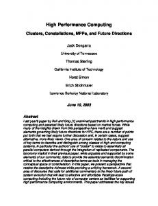
Fig. 2 CG Performance for different matrices and different number of nodes.
our hierarchical partitioning model by comparing internode communication volumes with correct and scrambled GPU mapping for partitioning result. Here, scrambled GPU mapping means, after the first phase of hierarchical partitioning, sub-submatrices obtained after decomposition of each submatrix are assigned to different nodes, instead of assigning them to the same node. For 16 nodes, each node having 2 GPUs, by scrambling the GPU mapping of submatrices acquired via recursive hypergraph partitioning, inter-node communication volume increases by more than 50%, while total communication volume among all GPUs remains the same. In this work, we only explain 1D rowwise matrix decomposition. Although we have thought other alternatives such as 2D partitioning models[6], our experiments suggest that rowwise decomposition is the simplest, yet the most effective solution amongst the ones we have thought.
5 Experimental results We evaluate performance of proposed CG algorithm on a set of multi-GPU nodes of TSUBAME supercomputer[15,16]. Each node of TSUBAME has 8 AMD 2.4 GHz Opteron dual core processors, 2 NVIDIA Tesla GPUs and 32 GB of main memory. We use 1 CPU (2 cores) from each node in our multi-GPU cluster experiments, where each core runs one thread and is responsible for controlling one GPU. Each Tesla GPU contains 30 streaming multiprocessors, each with 8 cores (240 cores in total) and 4 GB of device memory. Nodes are connected with high speed 4x SDR InfiniBand dual rail network, providing 20 Gbps bandwidth per node. Linux version 2.6.16 OS is installed on nodes. C++ programming language is used for coding. CUDA version 2.2 is
used for programming GPUs, pthread library is used for CPU threading and Voltaire MPI is used for MPI communication between nodes. For partitioning hypergraphs, recursive multilevel partitioning tool PaToH[5] is used, which runs sequentially on the CPU. 11 unstructured sparse matrices that are symmetric and positive definite with real value entries from Sparse Matrix Collection of University of Florida[20] are used for performance evaluation. Matrix dimensions vary from 63,838 to 1,585,478 and number of nonzeros varies from 5,080,061 to 77,651,847. The sparsest matrix has 4.8 nonzeros per row and the densest has 221.6 nonzeros per row, on average. Hypergraph partitioning is executed before CG solver as a preprocessing for efficient parallel multi-GPU solver. The preprocessing cost for hypergraph partitioning is amortized during CG iterations. The preprocessing cost for 8-way hypergraph partitioning is worth 35 to 180 sequential double precision CG iterations on the CPU for the matrices in our dataset. Double precision solver performance in Gflops using hierarchical hypergraph partitioning is given in Figure 2. In the figure, we compare sequential and parallel solver performances. 1 GPU denotes sequential performance using single GPU and n × 2 GPUs denotes performance on n nodes, each having 2 GPUs. Matrices are sorted according to the number of nonzeros they contain on x axis. For each CG iteration, executing 1 MxV and 5 vector operations, 2 × nnz + 10 × n flops are counted, where nnz is the number of nonzeros and n is the dimension of the matrix. Gflops is the count of billions of flops per second. Numbers annotated with bars of each matrix is the number of iterations required for CG to converge when ε = 10−10 . As seen in the figure, up to 119 Gflops of CG performance is achieved. Bigger matrices better scale with the
7
increase in number of nodes, because workloads become insufficient to utilize GPU resources for smaller matrices and communication time dominates. Reduction of communication time is the most important factor for performance. Several factors affect inter-node communication time, such as system dependent latencies and application dependent communication number and volume. We can control application dependent values and particularly in this work, we reduce total communication volume. For ldoor matrix, which we obtain best CG performance on 16 nodes, only 26,859 words are communicated between nodes for input vector of MxV, where the dimension of this matrix is 952,203. Local and coupling MxV computation times (excluding communication time) cost 35% of total solution time for this instance. For crankseg 2, which reveals the worst performance, 117,127 words are communicated between 16 nodes, where the dimension of this matrix is 63,838. For this instance, total MxV computation time takes 23% of total solution time. Note that, crankseg 2 is our densest matrix and variation of number of nonzeros within rows for this matrix is very high, which are two main reasons for relatively higher communication volume incurred. For the smallest matrix in the dataset, tmt sym, the ratio of MxV computation time to total time is 15% and for the biggest matrix, audikw 1, the ratio is 37%, on 16 nodes. These numbers confirm that as the matrix gets smaller with increasing number of GPUs, communication time dominates. Chosen MxV kernel is another factor that affects the performance of the solver. We observed that for all 11 matrices, HYB is the fastest sequential MxV kernel. However, on 16 nodes, it is interesting to observe that none of the GPUs select HYB as its MxV kernel, for all matrices. For 8 matrices all 32 GPUs select JDS-based kernel, for 2 matrices all GPUs select CSR vector kernel and for inline 1 matrix 25 GPUs select JDS-based kernel and 7 GPUs select CSR vector algorithm. Hence, as demonstrated, HYB kernel is effective sequentially, but it is not desirable for rowwise parallelization. The reason for that is not the partitioning techniques that we have explained, but decomposition itself. During our experiments with a set of matrices that we do not report all of them in this section, we have found out that HYB performance is worse for smaller matrices. In Figure 3, we demonstrate effectiveness of hypergraph partitioning (HP) and MxV kernel selection for multi-GPU clusters to obtain speedups, and make strong scaling comparisons of multi-GPU cluster with CPU clusters. We present results for two characteristic matrices. For the GPU implementation which does not utilize hypergraph models, nonzeros of the matrix are evenly distributed across GPUs by simply dividing the
Fig. 3 CG performance comparisons of proposed GPU cluster implementation with CPU cluster implementations using hypergraph models and alternative GPU cluster implementations.
matrix rowwise into equal nonzero sizes and vector entries are conformably distributed. As seen in the figure, simple decomposition with equal nonzero sizes does not yield almost any speedup, while using hypergraphpartitioning-based model, we can obtain considerable speedups. Auto-selection of MxV kernel is another factor that increase performance of the multi-GPU solver. For the case that auto-selection is not applied, best sequential GPU MxV kernel (HYB) is used in multi-GPU solver. As can be seen from the figure, best sequential MxV kernel does not scale for large number of GPUs. This deficiency is very severe for crankseg 2 matrix, because of its very irregular nonzero distribution. We used largest symmetric and positive definite matrices from the University of Florida Sparse Matrix Collection; however sizes of the matrices other than the largest one, audikw 1, are still insufficient to obtain speedups for 32 nodes over 16 nodes. Performance of the solver is bounded by the network communication for large number of nodes. We demonstrate this by comparing CG performance on GPU cluster with CPU cluster on TSUBAME using exactly same network between nodes, while theoretical peak flops per node is completely different. Double precision peak performance of 16 CPU cores in a node is 76.8 Gflops and 2 GPUs in a node is 172.8 Gflops. For CPU implementation, pthread library is used for parallelization among cores within a node. As in the GPU case, only one thread from each node is responsible for non-blocking MPI communication. Communication is minimized using hi-
8
erarchical partitioning as explained for multi-GPU clusters. Hence, using two cores per node, exactly same submatrices are assigned to CPU cores, instead of GPUs, and total communication volume between cores is the same with the multi-GPU cluster implementation. Regardless of the number of cores per node, inter-node communication volume is the same, using hierarchical partitioning. We experiment double precision CG with 2 and 16 CPU cores per node. Hence, we use up to 512 CPU cores from TSUBAME. Because of the space constraint, in Figure 3, we present results only for two characteristic matrices, but performance features for other matrices are similar. Without using hypergraph partitioning –although smaller than using hypergraph models– speedups can be obtained for only a few matrices, whose nonzeros are mostly already ordered around the diagonal. Without using kernel selection, multi-GPU solver scales worse for number of GPUs more than 4 to 8. For 2 GPUs/node and 16 CPUs/node, performance saturates around 16 to 32 nodes. Performance scales better for 2 CPU cores per node, because the computation can still be considered as slow compared to network communication time. CPU cluster performance is always below of the proposed multi-GPU cluster performance with the same underlying network. For all matrices, average CG performance is 11.5 Gflops for 64 CPU cores, 31 Gflops for 512 CPU cores and 46 Gflops for 64 GPUs on 32 nodes. To demonstrate effectiveness of our mixed pthread /MPI implementation over assigning one MPI process for each GPU, we have implemented the flat MPI model. We have found out that for 32 GPUs on 16 nodes, flat MPI implementation is slower than mixed model by 33%. For 16 nodes of GPU cluster, peak performance is around 2.76 Tflops, where we achieve up to 119 Gflops, only 4.3% of the theoretical peak. For single GPU, we achieve up to 10.8 Gflops performance over 172 Gflops theoretical peak, which is around 6.3% of the peak. This is because performance of the sparse solver is bounded by the peak memory bandwidth, instead of peak flops. Actually, we achieve up to 101 GB/s effective memory bandwidth using texture cache memory on single GPU, whose theoretical device memory bandwidth is 102.4 GB/s. Assuming cache hit rate of 100%, we achieve device memory bandwidth up to 65 GB/s on single GPU. In other words, we achieve between 63% to 99% device memory bandwidth utilization for single GPU. For 16 nodes and 32 GPUs, our peak effective memory bandwidth utilization is 1112 GB/s using texture cache. Assuming 100% cache hit rate, we achieve up to 716 GB/s device memory bandwidth utilization, which is around 22% for theoretical peak of 3.3 TB/s.
6 Conclusion We have explained a scalable implementation of Conjugate Gradients for unstructured matrices on multiGPU clusters. Although we have explained proposed techniques on a CG solver, they can be easily adopted to other iterative solvers for unstructured sparse matrices. Network communication is bottleneck in performance of parallel sparse solvers on traditional clusters. Interconnection between compute nodes of a GPU cluster –compared to fast GPU computation units– is even much slower for obtaining scalability. However, we have shown that scalability can still be obtained by matrix decomposition techniques based on hypergraph partitioning. To reduce inter-node communication size, we have explained a hierarchical partitioning model for correct mapping of decomposed matrices to GPUs. Each GPU selects the most appropriate kernel that runs during iterations for the matrix it processes. Experimental results confirm the validity of proposed techniques. We have presented strong-scalability experiments for well known matrices and discussed communication bottleneck for large number of nodes. Acknowledgements This research is partially supported by CREST project “ULP-HPC: Ultra Low-Power, High Performance Computing via Modeling and Optimization of Next Generation HPC Technologies” of Japan Science and Technology Agency (JST).
References 1. Baskaran, M. M. and Bordawekar, R.: Optimizing Sparse Matrix-Vector Multiplication on GPUs, IBM Research Report, RC24704 (2008). 2. Bell, N. and Garland, M.: Implementing Sparse MatrixVector Multiplication on Throughput-Oriented Processors, Proc. SC ’09: ACM/IEEE Conference on Supercomputing, Portland, OR, USA (2009). 3. Buatois, L., Caumon, G. and L´ evy, B.: Concurrent Number Cruncher: An Efficient Linear Solver on the GPU, Proc. HPCC 2007, LNCS 4782 , pp. 358–371 (2007). 4. Catalyurek, U. V. and Aykanat, C.: HypergraphPartitioning-Based Decomposition for Parallel SparseMatrix Vector Multiplication, IEEE Transactions on Parallel and Distributed Systems, Vol. 10, No. 7, pp. 673–693 (1999). 5. Catalyurek, U. V. and Aykanat, C.: A Multilevel Hypergraph Partitioning Tool, V. 3.0, Tech. Rep., Dept. of Comp. Eng., Bilkent University (1999). 6. Catalyurek, U. V., Ucar, B. and Aykanat, C.: On TwoDimensional Sparse Matrix Partitioning: Models, Methods, and a Recipe, Tech. Rep., OSUBMI-TR 2008 2008 n04 . 7. Che, S., Li, J., Sheaffer, J. W., Skadron, K. and Lach J.: Accelerating Compute Intensive Applications with GPUs and FPGAs, Proc. IEEE Symposium on Application Specific Processors (SASP) (2008). 8. Cevahir, A., Nukada, A. and Matsuoka, S.: Fast Conjugate Gradients with Multiple GPUs, Lecture Notes in Computer Science, Vol. 5544, Springer, pp. 898–903 (2009).
9 9. Fan, Z., Qiu, F., Kaufman, A. and Stover, S. Y.: GPU Cluster for High Performance Computing, Proc. SC04: ACM/IEEE Conference on Supercomputing (2004). 10. G¨ oddeke, D., Strzodka, R., Mohd-Yusof, J., McCormick, P., Buijssen, S. H. M., Grajewski, M. and Turek, S.: Exploring weak scalability for FEM calculations on a GPU-enhanced cluster, Parallel Computing, Vol. 33, No. 10–11, pp. 685– 699 (2007). 11. GraphStream Inc.: GraphStream Scalable Computing Platforms, http://www.graphstream.com (accessed 2009). 12. Harris, M.: Optimizing Parallel Reduction in CUDA, NVIDIA Developer Technology (2007). 13. Hartley, T. D. R., Catalyurek, U. V., Ruiz, A., Ujaldon, M., Igual, F. amd Mayo, R.: Biomedical Image Analysis on a Cooperative Cluster of GPUs and Multicores, Proc. 22nd ACM International Conference on Supercomputing, pp. 15– 25 (2008). 14. Lengauer, T.: Combinatorial Algorithms for Integrated Circuit Layout , Wiley, Cichester, UK (1990). 15. Matsuoka, S.: The Road to TSUBAME and Beyond, Petascale Computing: Algorithms and Applications, Chapman & Hall Crc Computational Science Series, pp. 289–310 (2008). 16. Matsuoka, S., Aoki, T., Endo, T., Nukada, A., Kato, T. and Hasegawa, A.: GPU-accelerated Computing – From Hype to Mainstream, the Rebirth of Vector Computing, J. Physics: Conference Series 180 , (2009). 17. NVIDIA Corporation: NVIDIA CUDA Compute Unified Device Architecture Programming Guide (2007). 18. Saad, Y.: SPARSKIT: A Basic Tool Kit for Sparse Matrix Computation, Tech. Rep. CSRD TR 1029 , University of Illionis, Urbana, IL (1990). 19. Teresco, J.D., Faik, J. and Flaherty J.R.: Hierarchical Partitioning and Dynamic Load Balancing for Scientific Computation, Proc. PARA’04 , pp. 911–920 (2004) 20. University of Florida Sparse Matrix Collection, http://www. cise.ufl.edu/research/sparse/matrices/.