Nov 18, 2011 - floating point power. Finally, the third challenge ... Wilson-Dslash operator, which on a single-socket, six-core West- mere CPU delivers close ..... In reality they will be implicitly loaded into LLC during ac- cess in Wilson-Dslash.
High-Performance Lattice QCD for Multi-core Based Parallel Systems Using a Cache-Friendly Hybrid Threaded-MPI Approach Mikhail Smelyanskiy1 , Karthikeyan Vaidyanathan1 , Jee Choi4 , Bálint Joó2 , Jatin Chhugani1 , Michael A. Clark3 , Pradeep Dubey1 1 3
Parallel Computing Labs, Intel 2 Thomas Jefferson National Accelerator Facility Harvard-Smithsonian Center for Astrophysics 4 Georgia Institute of Technology
ABSTRACT Lattice Quantum Chromo-dynamics (LQCD) is a computationally challenging problem that solves the discretized Dirac equation in the presence of an SU(3) gauge field. Its key operation is a matrixvector product, known as the Dslash operator. We have developed a novel multicore architecture-friendly implementation of the Wilson-Dslash operator which delivers 75 Gflops (single-precision) R R on an Intel Xeon Processor X5680 achieving 60% computational efficiency for datasets that fit in the last-level cache. For datasets larger than the last-level cache, this performance drops to 50 Gflops. Our performance is 2-3X higher than a well-known implementation from the Chroma software suite when running on the same hardware platform. The novel implementation of LQCD reported in this paper is based on recently published the 3.5D spatial and 4.5D temporal tiling schemes. Both blocking schemes significantly reduce LQCD external memory bandwidth requirements, delivering a more compute-bound implementation. The performance advantage of our schemes will become more significant as the gap between compute flops and external memory bandwidth continues to grow. We demonstrate very good cluster-level scalability of our implementation: for a lattice of 323 × 256 sites, we achieve over 4 Tflops when strong-scaled to a 128 node system (1536 cores total). For the same lattice size, a full Conjugate Gradients Wilson-Dslash operator, achieves 2.95 Tflops.
1.
INTRODUCTION
Lattice Quantum Chromo-dynamics (LQCD) is the lattice discretized theory of the strong force, that which binds together quarks in the nucleon. In LQCD, the propagation of quarks is given by the inverse of a large, sparse matrix known as the Dirac operator. Hence, many systems of linear equations must be solved involving this matrix; it is this requirement that makes LQCD a grand challenge subject. In such linear solvers, the application of the Dirac operator to a vector is the most compute intensive kernel. On the other hand, modern central processing units (CPUs) have continued to evolve, as the number of on chip transistors continues to grow. Their compute capacity has increased through progres-
Permission to make digital or hard copies of all or part of this work for personal or classroom use is granted without fee provided that copies are not made or distributed for profit or commercial advantage and that copies bear this notice and the full citation on the first page. To copy otherwise, to republish, to post on servers or to redistribute to lists, requires prior specific permission and/or a fee. SC11 November 12-18, 2011, Seattle, Washington, USA Copyright 2011 ACM 978-1-4503-0771-0/11/11 ...$10.00.
sively higher core counts and, more recently, wider Single Instruction Multiple Data (SIMD) vector units. Current CPUs feature between 6-8 cores on the same die. SIMD units have increased from 128-bit SSE to 256-bit AVX [16]. Thus comes the first challenge of efficiently utilizing available compute resources. However, memory bandwidth is increasing at a slower rate than compute capability. To reduce bandwidth requirements of memory intensive applications, such as LQCD, modern architectures feature large on-die caches, with capacities of O(10) MB. The second challenge is how to take full advantage of these caches, which may require changing the algorithm to improve data reuse, otherwise the algorithm will not be able to take full advantage of the available floating point power. Finally, the third challenge is parallelizing the algorithm on large scale systems, on which LQCD computation is usually deployed. In this paper we address all three challenges. Specifically, we develop a highly optimized single precision implementation of the Wilson-Dslash operator, which on a single-socket, six-core Westmere CPU delivers close to 75 Gflops of performance for datasets which fit into last level cache (LLC). Furthermore, we apply a recently published 3.5D spatial and 4.5D temporal blocking scheme to QCD, which takes full advantage of large LLC available on modern CPUs [25]. For large realistic datasets, which do not fit into LLC, our 3.5D blocking scheme achieves close to 42 Gflops performance on a single-socket CPU which is within 13% of the achievable memory bandwidth. We further show that in cases where Wilson-Dslash operators are applied consecutively, as in the context of an even-odd preconditioned linear operator, such as one would use in a Krylov subspace solver like Conjugate Gradients [12], we can apply a 4.5D blocking scheme to take advantage of the temporal locality between these operators to further reduce WilsonDslash bandwidth requirements. This scheme, allows us to achieve up to 50 Gflops on a single socket. In addition, we show that the advantages of the 4.5D scheme will continue to increase as the gap between memory bandwidth and compute density is expected to widen in the next generation architectures. Lastly, we demonstrate that our Wilson-Dslash implementation shows good scaling to multiple nodes. For a problem of volume 323 × 256 sites our implementation achieves over 4 Tflops when strong scaled to a 128-node (1536 cores) cluster. Throughout this work we use as a reference the Wilson-Dslash implementation distributed with the Chroma [10] software suite for LQCD. In our single-socket implementation, for problems that fall outside LLC and in our multi-node implementation we typically outperform the reference implementation by a factor of 3X. In the single-socket case, where the problem does fit into LLC the performance advantage in favor of our implementation is 2X.
Figure 1: Example of 2D lattice with even-odd labelling The rest of this paper is organized as follows. In Section 2 we present basic details of Wilson-Dslash, as well as our experimental environment. Section 3 provides details of our implementation. Section 4 presents performance results and analysis. We consider previous and related work in Section 5. Finally, we conclude and present our future work in Section 6.
2.
BACKGROUND
2.1 Lattice QCD LQCD is a formulation of QCD amenable to calculations on computers. It is a relativistic quantum field theory describing the interaction of quarks which are mediated by gauge bosons known as gluons. A full description of LQCD is beyond the scope of this work and the reader is referred to excellent textbooks on the subject [9, 27, 24]. Details of the QCD interactions are captured in the differential operator which couples quarks to the gluons. In terms of numerical computation the key task is the solution of systems of equations involving this operator, known as the Dirac operator. In the standard prescription to move QCD from a continuum to a lattice, quark fields are placed on lattice sites and gluon fields are ascribed to the the links of the lattice connecting the sites. In particular, on the lattice, the gauge fields are represented as the parallel-transporters between the sites which are members of the SU(3) group. In other words, the gauge fields are represented as 3 × 3 complex unitary matrices of unit determinant ascribed to the lattice links. The quark fields are ascribed to the sites of the lattice. A naive first order finite difference discretization of the Dirac operator, however, results in the infamous fermion doubling problem and the need to avoid this has lead to several alternative definitions of the quark fields and the Dirac operator in LQCD. In the following work, we consider the Wilson formulation [32] where a secondorder difference is added to the first order one. This formulation requires the quark fields on the sites to be stored as 12 component complex vectors, where the 12 components are a product of 4 spin components and 3 color indices. The quark objects are also referred to as 4-spinors or just spinors. The Dirac operator; M; then looks like: M = 1 − κD, where κ is a real parameter related to the quark mass and D is the Wilson Dslash term: D=
� 1 4 µ µ† (1 − γµ ) ⊗Ux δx+ˆµ,x′ + (1 + γµ ) ⊗Ux−ˆµ δx−ˆµ,x′ . (1) ∑ 2 µ=1 µ
In the above Ux refers to the gauge link emanating from site x in
the µ direction, where µ is one of x, y, z or t. The δx±ˆµ Kroeneckerdelta symbols correspond to the use of the spinor from the neigh-� boring site in the positive/negative µ direction and the 1 ± γµ terms are projector operators acting on spin indices (but leaving color indices alone). The spin projectors reduce the effective number of spin�degrees of freedom from four to two. In particular, Pµ± = 1 ± γµ can be ± ± written as Pµ± = R± µ Qµ , where Qµ acting on a spinor reduces it to have only two spin components (of 3 vectors so 6 complex numbers). The gauge link matrix U then needs to be multiplied only with the two remaining 3-vectors making up the 2 spin components. The action of R± µ then reconstructs a four component repreµ sentation. Hence the operation Ux (1 ± γµ ) on a 4 spinor ψ is comµ ± ψ. The decomposition operators puted as: R± U χ with χ = Q µ x µ Q± µ typically involve 12 Flops, and permutations of the complex components or flipping their sign. The reconstruction operators R± µ only flip signs or permute complex components and have no floating point costs. It is typical to partition the lattice into sub lattices, which are referred to as either “even”, or “odd” respectively. Sites are considered “even” if their co-ordinates sum to an even number; or “odd” if instead the sum of their co-ordinates is odd. This is equivalent to a red-black checkerboard labeling of the lattice sites. We show, by way of an example, a 2D lattice in Fig. 1. The lattice has 6x4 sites. which are appropriately colored to reflect their parity (e.g. red for “even”, black for “odd”). In this 2D example, there are 2 gauge field links, emanating from each site in the positive direction: from odd to even as well as from even to odd. Effectively, each site has 4 links (8 in 4D): 2 (4 in 4D) in the positive and 2 (4 in 4D) in the negative direction. Note that the link in the negative direction for the site is defined as the positive link of its negative neighbor. Each odd (even) site is updated using 4 (8 in 4D) neighboring sites using all 4 (8 in 4D) links. It can be seen that a nearest neighbor operator such as D will gather sites of one parity (e.g. even) and write to sites of the other (e.g. odd). Hence it is customary to label the operator as Doe or Deo to indicate that it takes even sites to odd ones or odd sites to even ones respectively. An even-odd preconditioning then gives the preconditioned matrix operator: M˜ oo = 1oo − κ2 Doe Deo , which is the Schur complement of M acting only on one parity of the lattice (in this case the odd one). This is typically the operator one would use in a Krylov subspace solver such as Conjugate Gradients [12] or BiCGStab [30]. A high-level view of the Wilson-Dslash kernel is given in Figure 2. For each output site of the even (odd) sub-lattice, we gather neighboring spinors from odd (even) sub-lattice (Step 1). We then apply the appropriate spin projector for each neighbor, and multiply by the gauge link matrix connecting the target and source sites (Step 2, 3 and 4). Finally, for each neighbor we reconstruct the appropriate 4-spinor representation and accumulate the results together to form the output (Step 5). When performance is limited by memory bandwidth, gauge field compression may be employed [8], wherein only the first two rows of the color matrices are stored in device memory, and using unitarity, the third row is reconstructed in registers from complex conjugate of the cross product of the first two rows. Thus the Wilson-Dslash algorithm performs 1320 flops (480 fmadds and 360 fadds) and reads 1440 bytes of data, in single precision, when no gauge field compression is used. If 2-row gauge field compression is used, the algorithm performs 1656 flops (624 fmadds and 408 fadds) and reads 1248 bytes of data.
2.2 Intel Multi-core CPU
nodes, due to the extremely large number of floating point operations required (current simulations require O(10) Tflops/s years worth of computation). As a result, we have mapped our LQCD implementation to a multi-node cluster. In particular, we use a 128-node cluster. Each node consists of a dual-socket CPU with the same configuration to the one described in the previous section, except it runs at the frequency of 2.9GHz. The nodes are connected via an InfiniBand interconnect that supports a one-way latency of 1.5 usecs for 4 bytes, a uni-directional bandwidth of up to 3380 Million bytes/sec and bi-directional bandwidth upto 6474 Million bytes/sec. Such a system is typical of clusters used in the analysis phase of LQCD calculations and is similar to clusters deployed at Fermi National Accelerator Laboratory and Thomas Jefferson National Accelerator Facility as part of the National Lattice QCD Computational Facility project. The so called gauge generation phase of LQCD requires scaling to leadership scale facilities and to simulate scaling to such large partitions we have carried out weak scaling tests with local, per-node problem sizes such as those that would be expected when running on partitions of O(10,000) cores.
for each output site do for each of 8 neighbors do 1. Gather neighbor spinor (24 numbers) 2. Spin project from 4 to 2 spinor components (12 flops) 3. Load gauge matrix for neighbor direction (18 numbers or 12 with gauge compression) 4. Multiply the 2-spin components by the SU(3) link matrix (2x66=132 flops or 174 with 2-row gauge compression) 5. Reconstruct the result of 4 and accumulate to output spinor (24 numbers, 24 flops) endfor endfor
Figure 2: The structure of the Wilson-Dslash kernel.
3. QCD IMPLEMENTATION R
R
Our experimental testbed consists of a single-socket Intel Xeon R CoreT M i7 microarchiProcessor X5680, which is based on Intel tecture. Read Write Non-temporal write
LLC 122 32 n/a
DRAM 21 11 20
Table 1: Measured achievable bandwidth (in GB/s) for LLC R CoreT M i7. and memory on Intel This is an x86-based multi-core architecture, which provides six cores on the same die. Each core is running at 3.3GHz. The architecture features a super-scalar out-of-order micro-architecture supporting 2-way hyper-threading. In addition to scalar units, it has 4-wide SIMD units that support a wide range of SIMD instructions called SSE4 [17]. In a single cycle, it can issue a 4-wide floatingpoint multiply and add to two different pipelines. Compared to architectures which only have fused multiply-add unit, such as [19], it can achieve full hardware utilization, even in case when multiply and add can not be fused. Each core is backed by a 32 KiB L1 and a 256 KiB L2 cache, and all six cores share an 12 MiB last level L3 cache. Together, the six cores can deliver a peak performance of 158 Gflop/s of single-precision arithmetic using SSE. The system has 6 GiB DDR3 memory. It consists of three channels running at 1333 MHz, which can deliver 32 GB/s of peak main memory bandwidth. Table 1 summarizes the achievable bandwidth for both memory as well as last level cache (LLC). The data in the table was measured using a microbenchmark, similar to the one in [23]. Our results are also similar to the results reported in this work. Note that LLC read bandwidth is almost 4x higher than main memory read bandwidth and LLC write bandwidth. We can also see that the DRAM write bandwidth with regular (write back) stores is half the write bandwidth compared to using non-temporal stores.
2.3 Multi-node CPU Lattice QCD problems cannot normally be realized on just a few
Achieving high performance on modern CPU requires algorithms which take full advantage of its compute resources and memory hierarchy. In this section we describe our SIMD- and cache-friendly data lay-out and our implementation of the Wilson-Dslash operator.
3.1 Compute Kernel SIMD-friendly Data Lay-out: the data ordering typical in applications such as Chroma [10], running on a CPU, is to place the space–time site indices running slowest with the internal dimensions (color, spin, and real/imaginary) running fastest. The advantage of this layout is that accesses to nearest neighbors require fetching only a small number of cache lines. For example, accessing a spinor requires fetching at most three cache lines on our CPU. However such implementation constraints SIMD to be exploited within a single site, as done in [21, 14]. This approach will not scale to a wider SIMD on current and emerging architectures [19, 16] due to high overhead of shuffles and limited amount of data level parallelism (DLP). One SIMD-friendly lay-out is to create one stream per field (e.g. spinor, or gauge) component. Such a lay-out is also known as “structure of arrays” (SOA) [33]. Each stream length is equal to the number of lattice sites. This exposes large amount of DLP, wherein SIMD can be exploited across adjacent sites. However, the large number of streams (24 for spinors and 18 for gauges) can exhaust read and write buffers and cause TLB conflicts. Storing subset of components together, as done on GPU [8], requires gather support, which is not available on our CPUs. We propose novel SIMD-friendly ordering that exploits SIMD across sites, yet avoids two of the aforementioned problems. Specifically, we store NX spinors (or gauge fields) in an SOA format: one array per component. Here, NX is number of lattice sites in the X dimension. As the result, sites are stored contiguously in X for each field component. Now we can work on v sites using v-wide SIMD (v=4 in our case). This is illustrated in Fig. 3(a). The shaded regions show the components of the even spinors e14 − e17 suitable to be held in a vector registers, their neighbors o15 − o18 in the positive X (X+) direction, and the neighbors o24 − o27 in the positive Y (Y +) direction. As can be seen from the figure, accessing component of Y + direction, requires an aligned SSE load (MOVAPS) instruction. This
Figure 3: SIMD-friendly data layout: (a) NX spinors are stored contiguously for each component; (b) partition un-friendly data layout, (c) partition-friendly data layout. is true for all other directions, except for X which requires unaligned loads. The unaligned loads incur no extra penalty on our Intel Core i7 architecture, compared to aligned accesses, as long the data being loaded does not span two cache lines. Only when we are at the boundary do the accesses become non-contiguous, as they require data from the opposite boundary, due to periodic boundary conditions. We handle this situation as a special case by reading the scalar value and blending it with the other three values using the Packed Align (PALIGNR) instruction from the SSE4 instruction set.1 Partition-friendly boundary lay-out: While this lay-out exposes DLP across sites, it can result in fragmentation in situations where the lattice is partitioned along the X dimension. This can occur both in our 3.5D blocking scheme (see Section 3.2) as well as in a multi-node implementation (see Section 3.4). Figure 3b) illustrates the situation. Here the grid is divided into two sub-grids along X. Accessing neighbors in the X+ direction requires fetching a new cache line for each component. This will result is substantial amount of memory traffic. To avoid this, we store the boundaries in an array of structure (AOS) format for each partition, as shown in Figure 3(c). Now, accessing the neighbors only requires fetching at most 3 cache lines for all the spinor components. To access the boundary we use (PALIGNR) instruction, as described earlier. This adds a small overhead, most notably for very small sub-lattices where boundary accesses can not be amortized by the large amount of computation in the rest of the sites along the X dimension. Memory organization and single socket parallelization: Our implementation stores even and odd sub-lattices of both gauge and spinor fields in separate data structures. This reduces the stride between accesses and allows them to be easily captured with the hardware pre-fetcher. We exploit three-level parallelization of our code: within socket, across sockets in dual-socket node, and across nodes. Here we describe parallelization on a single socket, while Section 3.4 describes the other two. To parallelize the code for large problem sizes on a single socket, we divide a single XYZ slice among all the cores as evenly as possible. The cores then simultaneously work on one XYZ slice at a time before moving on to the next slice along T dimension. This maximizes data reuse 9 1 PALIGNR takes two registers, concatenates their values and pulls out a register length subset from the result starting at a specified offset.
of spinors in cache as discussed in the next Section 3.2. However, such partitioning increases the amount of inter-core communication due to shared boundary sites, compared to dividing the local 4 dimensional volume into equal contiguous chunks amongst the cores (as is done, for example in the reference implementation from Chroma). Note that inter-boundary communication happens between cores on the same socket and is therefore faster than communication across sockets. Furthermore, inter-boundary communication is amortized by the large amount of work within the Dslash kernel. Nevertheless, for smaller problem sizes which fit entirely into LLC the inter core communication becomes more significant and we take an approach similar to Chroma to reduce this overhead. Finally, we assign Simultaneous Multi-Threading (SMT) threads within a core to work on alternating NX lines. This increases the constructive data sharing among the SMT threads.
3.2 3.5D Blocking Figure 4(a) shows an example of the flow of our algorithm when computing a single Wilson Dslash gathering from odd-sites and writing to even ones for an example with 8 XY Z slices and periodic boundary conditions. In the rest of the paper, we refer to this algorithm as WDS1. Each step i computes slice SEi of the even sub-lattice. Columns 3-5 show three spinor slices from the odd sub-lattice required for this computation (from the previous, current and following values of T ). We see two of the slices are reused across two iterations. For example, SO1 and SO2 required by SE1 at time 1, are also required by SE2 at time 2. Columns 6 and 7 show corresponding gauge slices from odd and even sub-lattices required at each time step. We see that there is no re-use among gauges due to parity. Hence, in order to take advantage of spinor reuse in LLC, it must be large enough to hold at least two spinor slices. However this assumes a perfect LRU policy for cache eviction 2 as well as full associativity. Since modern caches implement pseudo-LRU and have limited associativity, we conservatively require the LLC to hold total of 5 slices, 3 spinor and 2 gauge slices, to guarantee full reuse of spinor slices across the iterations. We rely on streaming stores, which are available on modern CPUs, to write output spinors directly to memory, thus bypassing LLC. If the LLC can hold the required number of slices, every input spinor is only brought in once from memory. In the cases where the 9 2 Perfect LRU evicts the data from the cache as soon as it is no longer used.
Figure 4: Computation pipeline: (a) single dslash, (b) two dslashes combined with intermediate grid stored in LLC estimation κ3.5D in [25]) due to the spinor ghost layer is equal to dimx3.5D dimx3.5D −1
dim3.5D
dim3.5D
y z × dim3.5D × dim3.5D . Note that due to parity, there is −1 −1 y
z
only a single boundary spinor in both directions, compared with two boundary elements in case of seven-point stencil, for example. The redundant traffic is minimized when all blocking dimensions are the same and equal to q dim3.5D ≤ 3 C/(nsslices ∗ S + ngslices ∗ 4 ∗ G) (3) Note that κ3.5D redundant memory accesses refer only to the input spinor sub-lattice; accesses to the output spinors and the input gauge fields do not incur extra traffic. Hence the total redundant memory traffic is (S ∗ (1 + κ3.5D ) + S + 8 ∗ G)/(2 ∗ S + 8 ∗ G). Figure 5: Example of 3.5D blocking: (a) geometric view, (b) pseudo-code LLC is too small to hold the required number of XY Z slices, additional (redundant) memory traffic will result. To minimize this traffic, we apply 3.5D blocking [25] to Wilson-Dslash. Specifically, we perform 3D blocking within a full XY Z slice of size NX × NY × NZ and stream along the fourth dimension (T ), as shown geometrically in Figure 5(a). Figure 5(b) also shows the pseudo-code, which is the generalization of the example in Figure 4(a). For the clarity of exposition, we explicitly load XYZ spinor and gauge slices into LLC. In reality they will be implicitly loaded into LLC during access in Wilson-Dslash. Note also, as described in Section 3.1, computation proceeds in parallel on v sites using v-wide SIMD (v=4 in , and our case). Following the notation in [25], let dimx3.5D , dim3.5D y dim3.5D be the blocking dimensions in X, Y and Z of the spinor z sub-lattice, respectively. We refer to the block region with these dimensions in each XYZ slice as an XYZ sub-slice. To capture the reuse of two sub-slices, we require that (nsslices ∗ S + ngslices ∗ 4 ∗ G) ∗ dim3.5D ∗ dimy3.5D ∗ dimz3.5D ≤ C (2) x Here C is the size of the LLC, and nsslices and ngslices are the minimum number of required XY Z spinor and gauge slices that the LLC must hold to guarantee spinor reuse. The factor of 4 is due to the fact that odd (even) gauge slice contains 4 gauges per site, one in each direction. The parameters S and G are the sizes of an individual spinor (96 bytes in SP) and gauge link matrix (48 bytes in SP when 2 row compressed, 72 when uncompressed), respectively. Once all sub-slices are in the LLC, the computation can be performed on an (dim3.5D − 1) × (dimy3.5D − 1) × (dimz3.5D − 1) × NT x sub-lattice, so that each spinor is only fetched once from memory. Spinors within the boundary spinors (referred to as the ghost layer) will be fetched twice, once for each sub-slice. Thus the amount of redundant traffic from memory (referred to as the over-
3.3 4.5D Blocking In the previous section, we showed how to minimize memory traffic in the Wilson-Dslash by capturing the reuse between spinors in the input sub-lattice. However, as Figure 4(a) showed, there is no reuse of the gauge fields. Note that in a real calculation the Dslash operator forms part of the preconditioned Dirac operator M˜ = 1 − k2 Doe Deo wherein the Dslash kernel is applied twice. The first application maps a spinor from an odd sub-lattice to a temporary even sub-lattice, and the second one maps this temporary sub-lattice back to the odd sub-lattice. We refer to two such applications of Dslashes as WDS2 in the rest of the paper. Note the temporary sub–lattice is not required outside this operation. As the result, it does not need to be written back to memory and therefore can be held in LLC. Gauges can also be reused, as explained next. Figure 4(b) shows an example combining two Dslash operations for NT = 8. At each step t we compute the t-th SEtmp slice (the result of applying the first Dslash) which requires three spinor slices from the old sub-lattice, as shown in the columns 4-6. At the same time we also compute t − 2-th slice of the output Sout which requires SEtmp slices from three previous time steps already computed, as shown in the columns 7-9. The first application maps a spinor from an odd sub-lattice Sin to a temporary even sub-lattice SEtmp, and the second one maps SEtmp back to the odd sub-lattice Sout. Due to the fact that going from odd to even and even to odd sub-lattices exercises overlapping sub-sets of gauges fields, these are also re-used as shown in the last 4 columns of Figure 4(b). For example, positive and negative links G2oe and G3eo, required by SEtmp3 at t = 3, are also required by SEtmp0 at time 4 and SEtmp2 at time time 6. In summary, each step of the WDS2 algorithm does twice as much computation as WDS1, but with the same number of memory accesses. However, for this up to 14 slices, 7 for spinors and 10 for gauges, may need to fit into LLC in the worst case. To reduce redundant memory traffic which arises when the LLC
is too small to hold required number of XYZ slices, we further apply 4.5D blocking to Wilson-Dslash [25]. Specifically, we perform 4D blocking within XYZ slice, as well as across consecutive applications of Dslash, and stream along the fourth dimension (T ). Note in this work we only combine two Dslash operators (blocking factor of two). To capture the reuse of both spinors and gauges, we use Equations 2 and 3, except that required number of spinors and gauge slices (nsslices and ngslices ) has increased. To estimate redundant memory traffic, note that WDS2 starts with dim4.5D × x XYZ slice, and after two application of Dslash, × dim4.5D dim4.5D z y only the data within (dim4.5D − 2) × (dimy4.5D − 2) × (dim4.5D − 2) x z XYZ sub-slice is correct. Hence redundant memory traffic κ4.5D is equal to
dimx4.5D dimx4.5D −2
dim4.5D
dim4.5D
y z × dim4.5D × dim4.5D . Since gauges are reused, −2 −2 y
z
they also incurs redundant memory traffic. Therefore, the total redundant memory traffic is (S + (1 + κ4.5 ) ∗ (S + 8 ∗ G))/(2 ∗ S + 8 ∗ G). There are several ways to parallelize the 4.5D computation. The simplest is to assign each of the slices, SEtmp and SOout to a nonoverlapping subset of cores. The problem with this implementation is that it would create a load imbalance, because as explained earlier, computing SEtmp takes all of its input data from memory, while computing SOout takes all of its input data from LLC. To address this problem, computation of SEtmp slice is merged with the computation of SOout slices. The work is further evenly divided among all the cores, such that each core works on a portion of both slices simultaneously. This way each core will perform roughly the same number of accesses to both LLC as well as memory. Also note, that due to the reuse of SEtmp, we require a barrier synchronization after every step. The overhead of synchronization is not an issue for larger data sets, because in these cases there is enough work per thread to amortize the overhead. The barrier overhead can limit the scalability for smaller datasets. However, small datasets typically fit into LLC and in such cases there is little advantage to be gained from using the WDS2 approach.
3.4 Scaling beyond one socket To scale the WDS1 and WDS2 implementations across multiple sockets within a node, we partition the Dslash grid across sockets and use the OpenMP (OMP) model for parallelization. For scaling across nodes, we use the Message Passing Interface [22] (MPI) model. With the migration of memory controllers (MC) on-chip (per socket), modern processors are subject to non-uniform memory access (NUMA) latencies. Fetching the data from the local MC is faster than accessing the remote MC. To achieve best performance, minimizing accesses to remote MCs is critical. Operating systems map memory in different MCs based on a first touch policy, i.e., the data is mapped to a particular MC if the request to touch the data for the first time is initiated from that MC. Our approach uses this policy to partition the Dslash grid (spinor and gauge) equally across sockets. First, we affinitize the OpenMP threads to hardware threads in the following order: threads per core, cores per socket and sockets per node. Next, we pick all the OpenMP threads that are mapped to each socket and use it to initialize their portion of the Dslash grid. This process ensures that all threads on each socket fetch data from their local MC most of the time to process the internal volume. The remote MC is accessed only when these threads process the ghost region. For scaling across multiple nodes, we use a multi-dimensional partitioning and parallelization strategy based on the MPI model. Our approach follows the standard bulk synchronous computational pattern. Broadly, we partition the problem in all four dimensions
(T , Z, Y and X). Then, we identify the local surfaces (boundaries) to be shared amongst nodes and their corresponding neighbors in each dimension. Next, we exchange the boundaries through explicit message passing to the neighbors on each dimension. After receiving the boundaries, each MPI process concurrently calculates the Wilson-Dslash kernel as well as the linear solver on its own partition. Handling Multi-dimensional Partitioning: The simplest approach of scaling the Dslash operator is to partition the problem along one dimension, typically the longest one available which is most often (but not always) the time dimension. However, with the increasing number of nodes available in modern clusters, one-dimensional partitioning can limit the scaling capability only up to the size of the single dimension. On the other hand, partitioning the problem on multiple dimensions brings in many challenges. Firstly, the boundaries become non-contiguous and exchanging them raises additional issues such as packing the data at the source and unpacking the data at the destination using memory copies. Modern networks such as InfiniBand [15] have the ability to gather the data from non-contiguous buffers and send the data using scatter/gather operations. Using this capability, the MPI model supports features such as defining new data types to specify non-contiguous buffers with constant stride and avoid the need to perform explicit copying. This feature works well only for boundaries that belong to T and Z dimension partitioning. The boundaries for other partitions do not have a constant stride. In such cases, we explicitly pack the data at the source and unpack at the destination. In our implementation, we distribute the problem across the nodes using MPI processes. Each MPI process internally uses OpenMP threads to take full advantage of the cores as well as the cache. Next, we divide the problem along the time dimension (T ), because compared to dividing the problem along other dimensions, this has lower computation to communication ratio when T is large, common case in the lattices we studied. As number of nodes grows, T partition becomes smaller than other dimensions. In this case, we start partitioning the problem along Z, Y, and X, repeating the same process as needed. To seamlessly perform the Wilson-Dslash kernel on the local partition even on boundaries, we oversize the local partition to accommodate the boundaries (ghost layer) exchanged from neighboring nodes. During the exchange process, this buffer is either directly specified, if applicable. Otherwise, data is explicitly copied to the boundary especially for non-contiguous slices. Handling Overlap of Communication with Computation: To overlap communication with computation, we initiate the data transfer of boundaries and ghost layers using non-blocking send and receive MPI calls. While the underlying network performs the data transfer, we process the internal volume to achieve the desired overlap. Modern networks can accelerate this data transfer by directly placing the data in the receive buffer at the destination using DMA without the need for multiple buffering. However, the address of the destination buffer should be known to the sender before initiating the data transfer. Typical MPI implementations use a handshake message between the communicating processes to exchange the address of destination buffers. Thus, to achieve best overlap, it is critical that this handshake message reaches the sender before initiating the data transfer. One approach is to pre-post the receive buffers (potentially many such buffers) prior to the send operation. However, this can result in cases where a process may have posted its send before the receiving process has posted its receive, thereby not achieving the desired overlap. To achieve effective overlap of communication with computation even if processes go out-of-sync,
we exploit the non-blocking MPI_Iprobe feature, in addition to preposting the buffers, to periodically check for outstanding messages and initiate data transfers.
4.
PERFORMANCE RESULTS
In this section we evaluate the performance of both versions of Wilson-Dslash, WDS1 and WDS2, as well as a full Conjugate Gradients solver application for lattice QCD on a single socket Intel Core i7 processor (Intel microarchitecture code name Westmere) as well as multi-node system and analyze the measured results. We compare our performance results with the reference implementation from the Chroma software [10] suite running on the same system.
4.1 Expected Performance To help understand the performance of the Wilson-Dslash operator, we derive several bounds on achievable performance which are summarized in Table 2. Here and in the rest of the paper the reported performance numbers are effective Gflops that may be compared with implementations on other architectures. In particular, the nominal number of flops per lattice site is 1320, which does not include the extra work done in the SU(3) reconstruction when link compression is performed. Bounds Compute bound (WDS1) LLC bound (WDS1) DDR bound (WDS1) DDR bound (WDS2)
Compression 101 239 48 96
No Compression 126 186 37 74
Table 2: Compute, LLC and DDR performance bounds in Gflops on single socket. As mentioned in Section 3.1, uncompressed gauge Wilson-Dslash performs 480 fmadds and 360 fadds. The fadds only utilize 50% of floating point hardware. Since our implementation works on 4 sites, for uncompressed gauge fields we can achieve the computebound performance of 21 Gflops (= 4 sites*1320/((480+360) cycles/3.3 GHz)) on single core or 126 Gflops on 6-core system. This is 80% of the peak floating-point performance (see Section 2.3). Using compressed gauge fields, the code performs 624 fmadds and 408 fadds. Using similar calculation, as in case of full gauge, we derive a compute-bound performance of 17 Gflops on single core or 101 Gflops on 6-core system. This is 64% of the peak. The loss of efficiency comes from the extra work done in the SU(3) reconstruction. This bound is idealized and does not account for other overheads, such as register spills, address calculation, and instruction scheduling. Actual achieved compute-bound performance, which depends on these factors, will be lower. Let us assume, in the case of WDS1, that the entire lattice resides in memory. With perfect spinor reuse in LLC, there is only a single memory access for each piece of data. Therefore, not counting the flops for gauge decompression (these are ’extraneous’ flops), 1320 flops the memory-bound performance of WDS1 is (96+G×8)/R , bw +96/Wbw where Rbw and Wbw are the memory read and write bandwidths respectively, and G is the size of a gauge-field matrix: 48 bytes with compression and 72 without compression. Assuming non-temporal writes, used in our implementation, we plug corresponding values from Table 1. We find that memory-bound performance using compressed gauge fields is 48 Gflops. A similar computation for uncompressed gauge fields gives 37 Gflops. Similar analysis can be done for LLC-bound performance, when the entire lattice resides in LLC and spinors are reused in L2. Us-
Figure 6: Performance for small problems which fit into LLC. ing Table 1, we find, that based purely on the available LLC bandwidth, were flops available, the LLC-bound performance could be as high as 186 Gflops for compressed gauges and 239 Gflops for full gauges. However, in actuality there are not enough compute resources to sustain such a rate. Thus computation will be the limiting factor in performance for datasets which fit entirely into LLC. On the other hand, memory-bound performance is a bottleneck for datasets which do not fit into LLC. For WDS2, when temporal locality is exploited, the memory bandwidth is reduced by half for input spinor and gauge lattices. As the result, the memory-bound performance is twice that of WDS1. Specifically, it is 96 Gflops for compressed, and 76 for uncompressed gauge fields, respectively. The actual achieved performance, which we will talk about next, is limited by the above bounds. As before, memory-bound performance of WDS2 assumes unlimited flops. In reality, its performance is bound by compute, as will be shown in Section 4.3.
4.2 Small Problem Size In this section we provide the performance results and analysis for small problems which fit entirely into LLC. Such problems are important in the context of leadership class systems where the problem is partitioned among very large number of CPUs and the local problem becomes small enough to fit into the LLC of each CPU. Figure 6 shows performance for a range of small problem sizes. The middle bar shows the performance of the implementation using two row compressed gauge fields. For larger problem sizes, such as 8x8x8x32 sites, the performance reaches 72 Gflops. The black line shows the speed-up using 6 cores compared to a single one. For 8x4x4x4, the speed up is only 3.4X, which is low on 6-core system. This is due to inter-core communication. As the problem size increases, inter-core communication is reduced, compared to an increased amount of computation and the speed-up reaches over 5.4X for the 8x8x8x32 problem resulting in a single core performance of 13.3 Gflops/core. This is 80% of the achievable performance bound of 17 Gflops, derived in Section 4.1. The remaining 20% is overhead due to spills, fills, and register moves generated by the compiler to address high register pressure, inherent to the Wilson-Dslash implementation. We expect this overhead to be significantly reduced in AVX [16], which introduces non-destructive source operands. The left-most bars in Figure 6 shows the performance using uncompressed gauge fields. According to our model in Section 4.1, we expect this case to achieve 20% higher performance than when
using compression. However, we achieve only between 2%-9% higher performance, than the compressed case, with the highest achieved performance of 75 Glops for 8x8x8x32. This is due to extra loads required to load the third row of the uncompressed SU(3) matrix. These loads as well as loads that come from register fills put more pressure on a single load port and reduce benefits of uncompressed approach. On the other hand, Intel Core i7 has two ports for issuing floating point operations, which mitigates the overhead of row reconstruction in compressed approach. Note that for a problem of size 8x16x16x16, without compression, performance drops down to 50 Gflops, and becomes lower than the performance obtained using compression for the the same problem size. This is due to the fact that in this case, the problem size reaches the LLC capacity and starts resulting in an extra number of LLC evictions. The right bar shows performance of reference Chroma implementation. We achieve an average of 2X speedup over Chroma for LLC-bound problems. This is due to the fact that Chroma exploits SSE only within a single site. In addition, it incurs the overhead of run-time data rearrangement to convert data back and forth between native Chroma layout and the layout used by SSE code. Note that the performance of LLC-resident problems is lower than memory-bound performance of WDS2 scheme, which establishes a lower bound on is achievable performance of 75 Gflops, as opposed to 96 Gflops, projected in Section 4.1.
4.3 Large Problem Size In this section we present performance results for WDS1 with and without 3.5D blocking, as well as WDS2 with 4.5D blocking. We use four large lattices which do not fit into LLC of single CPU. Here and in the rest of the paper we use gauge compression. As discussed in Section 3.2, in the worst case, to guarantee spinor reuse in case of 3.5D blocking, LLC must hold 3 spinor and 2 gauge slices. While smaller number of slices is possible, we obtained our best resultsp using these number of slices. From Equation 3 we get dim3.5D = 3 12MiB/(4 ∗ 96 + 2 ∗ 4 ∗ 48) = 26. Redundant memory traffic for input spinors, κ3.5D evaluates to 1.12X. This corresponds to around 1.02X of redundant traffic for the entire problem. For 4.5D blocking, in the worst case, 7 spinors slices and 10 gauge slices are needed. Using the same equation, we compute find dim4.5D = 17. For this value of dim4.5D , κ4.5D is 1.46X, which translates to overall redundant memory traffic of around 1.38X. As LLC size continues to grow in future architectures, κ4.5D will decrease. For comparison, if size of LLC were to quadruple, κ4.5D would go down to 1.26 and overall redundant memory traffic would go down to 1.22X. Performance results are shown in Figure 7. First bar on the left shows WDS1 without 3.5D blocking. For the two smallest problems (163 × 64 and 243 × 128), we achieve close to 43 Gflops. This is 90% of the memory-bound performance of 48 Gflops (see Section 4.1). The 163 × 64 problem needs 3 MiB to reuse spinors, while 243 × 128 needs 9 MiB. This can be accommodated by 12 MiB LLC. As the result, no blocking is required. For the two largest problems (323 × 256 and 403 × 256), performance drops down to 36 Gflops and 30 Gflops, respectively. Note that 323 ×256 problem requires 22 MiB and the 403 × 256 requires 43 MiB to guarantee the reuse of spinors. This exceeds the capacity of LLC and results in additional memory traffic. Second bar shows performance of WDS1 with 3.5D blocking. As expected, for two smallest lattices, performance is the same as when no 3.5D blocking is used. For 323 × 256, performance has improved to 41 Gflops, which is 1.14X speedup over no 3.5D blocking performance on the same lattices. 403 × 256 performance has improved to 40 Gflops, which is 1.33X speedup over no 3.5D
Figure 7: Performance for large problems blocking. We also see that with 3.5D blocking, performance of WDS1 on two largest lattices is within 6% compared to two smallest problem sizes. The third bar shows performance of WDS2 scheme with 4.5D blocking. Performance has improved significantly in all cases. Compared to WDS1 without 3.5D, performance improved 1.24X for the smallest lattice and 1.6X for the largest lattice. Compared to WDS1 with 3.5D, performance has improved by 1.2X on average. While WDS2 can achieve up to 53 Gflops, its performance is lower than expected performance bound of 76 Gflops (see Table 2). The reason for this is as follows. As described in Section 3.3, our 4.5D implementation merges together computation of even and odd slices (Etmp and Oout in Figure 4(b)). While this improves load-balance, it decreases single-core performance to under 10 Gflops, compared to 13.3 Gflops reported in previous section. The decrease is due to several reasons. Firstly, there is an increase in L1 miss rate that comes from twice the number of lattice sites that must now be processed, as well as increase in register spills and fills due to higher register pressure. Secondly, there is an increase in I-cache miss rate, which comes from doubling code size, as the result of merging the computation. As the result, full system performance becomes bound by compute, reaching 53 Gflops. The right bar shows performance of Dslash reference code. Its performance does not vary much with lattices size and is about 3.4X slower than out 4.5D blocking scheme and 2.8X slower than 3.5D blocking. Note as the compute continues to scale at a faster rate then memory bandwidth, performance of 4.5D will improve. We demonstrate this with an experiment shown in Figure 8. Shown are four platform configurations of different byte:flop ratios, obtained by scaling up frequency and removing memory channels on our system. Left and right bars show performance of 3.5D and 4.5D configurations, respectively, while the line graph shows the 4.5D speedup over 3.5D schemes. Results are shown for 163 × 64 lattice. Second set of two bars shows performance on current configuration, as reported in Figure 7. 4.5D achieves 1.24 speedup over 3.5D. First set of bars shows performance on the CPU with the same memory bandwidth but slower compute (achieved by running at half the frequency). We observe that 4.5D has no benefit over 3.5D, as both schemes as compute bound. Third set of bars shows configuration with faster compute (overclocked to 4 GHz), but slower memory (1 channel removed). We see that 3.5D slowed down slightly, because it is bandwidth bound, while 4.5D improved, because it is com-
Figure 8: Performance scaling of 4.5D on 163 x64 lattices for different platform configurations.
pute bound. The fourth set of bars shows same configuration as the third with another memory channel removed (memory bandwidth is now reduced to 10 GB/s, while byte:flop ratio dropped to 0.06). As a result, the performance of 3.5D scheme has further decreased to almost half of the previous configuration, as expected. Moreover 4.5D has also decreased, as it is also now memory bound, however, it is close to 2X faster than 3.5D, because faster compute allowed 4.5D to run at full bandwidth capacity. Hence while 4.5D does not realize its full potential on current CPU, its performance will improve on future CPUs, as the number of cores continues to increase at a faster rate than memory bandwidth.
4.4 Multi-node Performance In this section, we describe the strong and weak scaling performance of our implementation across multiple nodes. As mentioned in Section 3.4, we use OMP model across sockets within a node and MPI across nodes. We found it to be 10% faster than using MPI across sockets within a node. For all experiments, we use the 128-node cluster system as described in Section 2.3. The version of icc compiler used for evaluations is 12.0.2 and we use Intel MPI [18] version 4.0.1.007. We extend the single-socket WDS1 implementation, optimized with 3.5D blocking, for the cluster. We refer to this scheme as WDS1-MPI. We compare its performance with the reference implementation from the Chroma software suite. We have also extended WDS2 scheme with 4.5D blocking for the cluster referred to as WDS2MPI. According to Section 4.3 WDS2 delivers 1.2X faster performance than WDS1 on 3.3GHz CPU. However, each CPU within the cluster runs at 2.9GHz, which reduces the benefits of WDS2 to only 5%. As the result, we omit results for WDS2-MPI from the performance results. As we pointed out in Section 4.3, as compute capacity continues increasing, WDS2-MPI will deliver up to the factor of 2 higher performance, compared to WDS1-MPI for problems which are not communication-bound. Figure 9 demonstrates the strong scaling performance for two problem sizes, 243 ×128 and 323 ×256, using two sockets per node (12 cores) up to 128 nodes (1536 cores). As Figure 9(a) and Figure 9(b) show, we achieve over 64 Gflops for a single node (dual socket). This is close to linear speedup over single socket running at 2.9GHz. In Figure 9(a), we see that the performance of WDS1MPI using the 323 × 256 lattice scales close to linear for up to 64
nodes. However, the efficiency drops to 50% on 128 nodes, which corresponds to 4 Tflops. For 243 × 128 lattice performance scales well up to 16 nodes, achieving only 30% efficiency on 128 nodes, which corresponds to 2.7 Tflops. The reason for the loss of linear scalability for both problem sizes is as follows. As the number of nodes increases, the problem size per each socket decreases. This exposes the overhead of copying and communicating boundaries. For example, for 243 × 128 lattice on 128 nodes 46% of communication overhead is exposed. For 323 × 256 lattice the overhead is 25% for the same number nodes. The rest of the overhead is due to boundary copying. Figures 9(a) and (b) also show that in most cases WDS1-MPI achieves more than a factor of two performance improvement as compared to Chroma for both the problem sizes. This improvement is due to faster computation, especially for smaller number of nodes, as demonstrated in Sections 4.2 and 4.3. The performance improvement for the larger number of nodes is due to the combination of faster computation and the use of non-blocking MPI_Iprobe feature, as described in Section 3.4: the feature currently not exploited in Chroma. Note however that the gap between Chroma and WDS1-MPI decreases, as number of nodes increases for both problem sizes. This is expected, as for large number of nodes both implementations become communication-bound. The weak scaling performance is shown in Figure 9(c). We see that both WDS1-MPI and Chroma show linear scaling up to 128 nodes for the 324 lattice. We also see that WDS1-MPI does not show significant performance benefits as compared to Chroma when using the 84 lattice. The reason being this lattice completely fits in the cache and becomes communication bound even on small number of nodes. Also, we observe that WDS1-MPI using the 324 lattice shows better performance as compared to the 84 lattice. This is expected, because 84 lattice has large and frequent amount of communication, compared to computation, which stresses the underlying network and increases the communication delay. Lattice 243 × 128 323 × 256
Nodes=32 994 821
Nodes=64 1466 1649
Nodes=128 1948 2951
Table 3: Performance of LQCD Parallel CG Solver. Finally, Table 3 demonstrates the performance of a QCD Conjugate Gradients (CG) solver using our Wilson-Dslash operator in an even-odd preconditioned Dirac operator, on both lattices. We see that the peak sustained performance is up to 3 Tflops for the 323 × 256 lattice. We also see that the CG solver has a 25% slowdown as compared to the peak sustained performance of the Wilson-Dslash kernel of 4 Tflops as shown in Figure 9(a). This slowdown is due to the additional computation incurred by the linear solver in level 1 BLAS operations and the synchronization overheads incurred in global reduction operations (global sums) performed across the MPI cluster. Although beyond the scope of this work, we note significant improvement would be obtained using a variant of pipelined CG [29].
5. COMPARISON WITH PREVIOUS WORK There are several implementations of LQCD Dslash implementations in the literature, many of them targeting novel architectures (of the time of their writing) such as GPUs [8, 1], the QCDSP supercomputer [6] or the QCDOC [4] and BlueGene/L supercomputers [31]. In particular [6] and [31] won Gordon Bell prizes for cost effective supercomputing in 1998 and 2006 respectively. The latest in the area of custom built machines is the QPACE computer [2]
2048 1024 512 256 128 64
1024 512 256 128 64 32
16
16 2
4
8 16 32 Number of Nodes
64
128
Chroma (32x32x32x32) WDS1-MPI (32x32x32x32) Chroma (8x8x8x8) WDS1-MPI (8x8x8x8)
4096
2048
32 1
8192
Chroma WDS1-MPI
4096 Sustained GFLOPS
Sustained GFLOPS
8192
Chroma WDS1-MPI
4096
Sustained GFLOPS
8192
2048 1024 512 256 128 64 32 16
1
2
4
8 16 32 Number of Nodes
64
128
1
2
4
8 16 32 Number of Nodes
64
128
Figure 9: Strong and weak scaling performance of Wilson-Dslash kernel on 128 nodes, 12 cores per node cluster: (a) strong scaling with 323 × 256 lattice, (b) strong scaling with 243 × 128 lattice, and (c) weak scaling. build using Cell processors, and Dslash implementations for the Cell are described in [28, 3] and [14]. Work with LQCD in commodity clusters is discussed in [13] and [11]. However, both these contributions come from before the era of multi-core CPUs with large shared caches such as considered here, and the prime focus was on exploiting the SSE registers and using aggressive prefetching to hide memory latencies or to find the correct combination of commodity components to produce the most cost effective system in terms of Flops/$. The first use of SSE vectorization in QCD was reported by [20]. In [5] and [26] code generators are presented to aid the user in making use of architectural features. In [5] the code generator simulates pipelines on a variety of RISC architectures, provides register and floating point abstractions to the user and can generate code for a variety of architectures. This has proved very fruitful on both the QCDOC and BlueGene architectures. Memory abstractions are in terms of streams and the code generator takes care of memory prefetching to provide efficient streaming and strided memory access. Managing cache and reuse are still left to the user of the package. The author of [5] also makes available a Wilson-Dslash package (BAGEL Wilson Dslash) which provides high performance on QCDOC and BlueGene architectures. The most recent evolutions feature a hybrid multi-threaded MPI approach. However, we do not know how shared caches are handled. In [26] a register transfer language (QA0) is described. The QA0 compiler can then generate efficient code from code written in the QA0 language on a range of back ends. Again, cache management is left to the user, however the authors describe their MDWF package for implementing the domain-wall formulation of Dirac Operator. In this package, the site ordering comes from a cacheoblivious, successive recursive bisection of the lattice along its dimensions. The resulting domain-wall Dirac operator achieves high performance and excellent weak scaling BlueGene & P architectures. The reference Dslash is an offshoot of the one described in [21], which was originally crafted from the freely available code from Martin Lüscher [20]. The reference code had incorporated threading through either OpenMP or the QMT [7] lightweight threaded library. However the lattice is always divided amongst threads lexicographically and no cache blocking is performed. Further, the multi-node version of the code is performed with a different structure, which has more memory traffic than the work presented here. Correspondingly, while the reference Dslash should perform comparably to WDS1-MPI (and does, see Fig. 9(a) at 1536 cores) at the strong scaling limit when the local problem size is small, it is expected that the better cache reuse in the work presented here should result in much better performance for larger local volumes (this too is borne out in the previous section).
6. CONCLUSIONS AND FUTURE WORK In this work, we developed a highly optimized single-precision implementation of the Wilson-Dslash operator which on singlesocket CPU delivers close to 75 Gflops of performance for datasets which fit into last level cache (LLC). This is more than 2X faster than the reference implementation available to us running on the same system. Furthermore, we have applied recently published 3.5D blocking scheme to QCD, which takes full advantage of large last level cache (LLC) available on modern CPU. For large realistic datasets, which do not fit into LLC, our implementation achieves over 42 Gflops performance on a single socket CPU. This is close to 90% of achievable memory bandwidth and is more than 2.5X faster than the reference Chroma implementation of Wilson-Dslash running on the same system. We further show that in cases where two Wilson-Dslash operators are applied consecutively, as in the context of a preconditioned linear operator, we can take advantage of the temporal locality between these operators to further reduce memory bandwidth requirements. This scheme, called 4.5D, allows us to achieve close 50 Gflops on a single socket. While this turns QCD into compute-bound problem, its performance is limited by overheads. However, we also show that advantage of the 4.5D scheme will continue to increase as the gap between memory bandwidth and compute density is expected to widen in the next generation of architectures. Lastly, we demonstrate that our Wilson-Dslash implementation is scalable. In particular for a problem of volume 323 × 256 problem our implementation achieves over 4 Tflops on a 128-node (1536 cores) cluster. This is more than 2X faster than our reference implementation running on the same system. For the same lattice size, a full Conjugate Gradients [12] solver using our implementation of Wilson-Dslash operator, achieves 2.95 Tflops. We believe that the techniques described here can be usefully employed in other architectures which feature multiple cores and large shared caches.
7. ACKNOWLEDGEMENTS Bálint Joó is funded through U.S. DOE project grants DE-FC0206ER41440 and DE-FC02-06ER41449 (USQCD SciDAC project) and DE-AC05-06OR23177 under which Jefferson Science Associates LLC manages and operates Jefferson Lab. The U.S. Government retains a non-exclusive, paid-up, irrevocable, world-wide license to publish or reproduce this manuscript for U.S. Government purposes. Michael A. Clark acknowledges funding under NSF grant OCI-1060067.
8. REFERENCES
[1] R. Babich, M. A. Clark, and B. Joó. Parallelizing the QUDA Library for Multi-GPU Calculations in Lattice Quantum
[2] [3] [4]
[5]
[6]
[7]
[8]
[9]
[10] [11]
[12]
[13] [14]
[15] [16]
[17] [18]
Chromodynamics. In Proceedings of the 2010 ACM/IEEE International Conference for High Performance Computing, Networking, Storage and Analysis, SC ’10, pages 1–11, Washington, DC, USA, 2010. IEEE Computer Society. H. Baier et al. QPACE – a QCD parallel computer based on Cell processors. PoS, LAT2009:001, 2009. F. Belletti et al. QCD on the Cell Broadband Engine. PoS, LAT2007:039, 2007. P. Boyle, D. Chen, N. Christ, M. Clark, S. Cohen, Z. Dong, A. Gara, B. Joo, C. Jung, L. Levkova, X. Liao, G. Liu, R. Mawhinney, S. Ohta, K. Petrov, T. Wettig, A. Yamaguchi, and C. Cristian. QCDOC: A 10 Teraflops Computer for Tightly-Coupled Calculations. In Proceedings of the ACM/IEEE SC2004 Conference, SC ’04, page 40, 2004. P. A. Boyle. The bagel assembler generation library. Computer Physics Communications, 180(12):2739 – 2748, 2009. 40 YEARS OF CPC: A celebratory issue focused on quality software for high performance, grid and novel computing architectures. D. Chen, P. Chen, N. H. Christ, R. G. Edwards, G. Fleming, A. Gara, S. Hansen, C. Jung, A. Kahler, S. Kasow, A. D. Kennedy, G. Kilcup, Y. Luo, C. Malureanu, R. D. Mawhinney, J. Parsons, C. Sui, P. Vranas, and Y. Zhestkov. Qcdsp machines: design, performance and cost. In Proceedings of the 1998 ACM/IEEE conference on Supercomputing (CDROM), Supercomputing ’98, pages 1–6, Washington, DC, USA, 1998. IEEE Computer Society. J. Chen and W. W. Iii. Multi-threading performance on commodity multi-core processors. In In Proceedings of 9th International Conference on High Performance Computing in Asia Pacific Region (HPCAsia, 2007. M. A. Clark, R. Babich, K. Barros, R. C. Brower, and C. Rebbi. Solving Lattice QCD systems of equations using mixed precision solvers on GPUs. Comput. Phys. Commun., 181:1517–1528, 2010. M. Creutz. QUARKS, GLUONS AND LATTICES. Cambridge, Uk: Univ. Pr. ( 1983) 169 P. ( Cambridge Monographs On Mathematical Physics). R. G. Edwards and B. Joo. The Chroma software system for lattice QCD. Nucl. Phys. Proc. Suppl., 140:832, 2005. A. Gellrich, D. Pop, P. Wegner, H. Wittig, M. Hasenbusch, and K. Jansen. Lattice qcd calculations on commodity clusters at desy, 2003. M. R. Hestenes and E. Stiefel. Methods of Conjugate Gradients for Solving Linear Systems. Journal of Research of the National Bureau of Standards, 49(6):409–436, Dec. 1952. D. J. Holmgren. PC clusters for lattice QCD. Nucl. Phys. Proc. Suppl., 140:183–189, 2005. K. Z. Ibrahim and F. Bodin. Efficient simdization and data management of the lattice qcd computation on the cell broadband engine. Sci. Program., 17:153–172, January 2009. InfiniBand Trade Association. 2004, http://www.infinibandta.org. Intel Advanced Vector Extensions Programming Reference. 2008, http://softwarecommunity.intel.com/isn/downloads/intelavx/IntelAVX-Programming-Reference-31943302.pdf. Intel SSE4 programming reference. 2007, http://www.intel.com/design/processor/manuals/253667.pdf. Intel Corporation. Intel MPI: Message-Passing Interface
[19] [20]
[21]
[22] [23]
[24]
[25]
[26] [27] [28]
[29]
[30]
[31]
[32]
[33]
Library. http://software.intel.com/en-us/articles/intel-mpi-library/. N. Leischner, V. Osipov, and P. Sanders. Fermi Architecture White Paper, 2009. M. Luscher. Schwarz-preconditioned HMC algorithm for two-flavour lattice QCD. Comput. Phys. Commun., 165:199–220, 2005. C. McClendon. Optimized lattice qcd kernels for a pentium 4 cluster. Technical Report JLAB-THY-01-29, Thomas Jefferson National Laboratory, 12000 Jefferson Ave, Newport News, VA 23606, USA, 2001. MPI: A Message-Passing Interface Standard. Mar 1994. D. Molka, D. Hackenberg, R. Schone, and M. S. Muller. Memory performance and cache coherency effects on an intel nehalem multiprocessor system. Parallel Architectures and Compilation Techniques, International Conference on, 0:261–270, 2009. I. Montvay and G. Munster. Quantum fields on a lattice. Cambridge, UK: Univ. Pr. (1994) 491 p. (Cambridge monographs on mathematical physics). A. D. Nguyen, N. Satish, J. Chhugani, C. Kim, and P. Dubey. 3.5-d blocking optimization for stencil computations on modern cpus and gpus. In SC, pages 1–13, 2010. A. Pochinsky. Writing efficient QCD code made simpler: QA(0). PoS, LATTICE2008:040, 2008. H. J. Rothe. Lattice gauge theories: An Introduction. World Sci. Lect. Notes Phys., 74:1–605, 2005. J. Spray, J. Hill, and A. Trew. Performance of a Lattice Quantum Chromodynamics Kernel on the Cell Processor. Comput. Phys. Commun., 179:642–646, 2008. R. Strzodka and D. Göddeke. Pipelined mixed precision algorithms on FPGAs for fast and accurate PDE solvers from low precision components. In IEEE Symposium on Field-Programmable Custom Computing Machines (FCCM 2006), pages 259–268, Apr. 2006. H. A. van der Vorst. Bi-CGSTAB: A Fast and Smoothly Converging Variant of Bi-CG for the Solution of Nonsymmetric Linear Systems. SIAM Journal on Scientific and Statistical Computing, 13(2):631–644, 1992. P. Vranas, G. Bhanot, M. Blumrich, D. Chen, A. Gara, P. Heidelberger, V. Salapura, and J. C. Sexton. The bluegene/l supercomputer and quantum chromodynamics. In Proceedings of the 2006 ACM/IEEE conference on Supercomputing, SC ’06, New York, NY, USA, 2006. ACM. K. G. Wilson. Quarks and Strings on a Lattice. In Zichichi, A., editor, New Phenomena in Subnuclear Physics, page 69. Plenum Press, New York, 1975. Y. Zhong, M. Orlovich, X. Shen, and C. Ding. Array regrouping and structure splitting using whole-program reference affinity. In Proceedings of the ACM SIGPLAN 2004 conference on Programming language design and implementation, PLDI ’04, pages 255–266, 2004.