1144
IEEE TRANSACTIONS ON SIGNAL PROCESSING, VOL. 54, NO. 3, MARCH 2006
High-Throughput Scalable Parallel Resampling Mechanism for Effective Redistribution of Particles Sangjin Hong, Senior Member, IEEE, and Petar M. Djuric´, Fellow, IEEE
Abstract—A novel resampling mechanism for parallel processing of fixed-point particle filtering is discussed. The proposed mechanism utilizes a particle-tagging scheme during quantization to compensate possible loss of replicated particles due to the finite precision effect. Particle tagging divides replicated particles into two groups for systematic redistribution of particles to eliminate particle localization in parallel processing. The mechanism utilizes an efficient interconnect topology for guaranteeing complete redistribution of particles even in case of potential weight unbalance among processing elements. The proposed architecture supports high throughput and ensures that the overall parallel particle filtering execution time scales with the number of processing elements employed. Index Terms—Fixed-point processing, parallel resampling, particle filters, residual resampling, scalable architecture.
I. INTRODUCTION
P
ARTICLE filters are used in nonlinear signal processing where the interest is in tracking and/or detection of random signals. Particle filters base their operations on representing relevant densities by discrete random measures composed of particles and weights and compute integrals by Monte Carlo methods [1]–[5]. More specifically, at every time instant , a random measure is defined, where is the th particle of the signal at time is the th trajectory of the signal, and is the weight of the th particle (or trajectory) at is time . If now, for example, an estimate of is a function of , the estimate can easily needed, where be computed using the random measure from (1) The particle filters have three important operations: generation of new particles, computation of the particle weights, and resampling. The resampling operation is very important for accurate tracking [6]–[9]. The idea of resampling is to remove the trajectories that have small weights and to focus on trajectories that are dominating. Standard algorithms used for resampling are different variations of stratified resampling [3], Manuscript received May 30, 2004; revised May 5, 2005. This work was supported by the NSF under Award CCR-0220011. The associate editor coordinating the review of this manuscript and approving it for publication was Prof. Chaitali Chakrabarti. The authors are with the Department of Electrical and Computer Engineering, Stony Brook University—SUNY, Stony Brook, NY 11794-2350, USA (e-mail:
[email protected];
[email protected]). Digital Object Identifier 10.1109/TSP.2005.863004
[10]. The two most common methods for resampling are systematic and residual resampling [1], [11], [12]. While these algorithms are very effective in particle filtering, physical implementation of such algorithms pose challenges especially when parallel processing is sought for large number of particles. When the number of particles, , becomes large, parallel processing of particle filtering is often considered to reduce its execution time of an iteration. There has not been any attempt for an effective parallel resampling mechanism in the research community. An efficient mechanism for single processing element (PE) in fixed-point processing of a particle filter has been previously discussed [13]. It has also been shown that the execution time of a fully pipelined particle filtering including resampling is , where is the total number of particles dedicated is the execution clock period. for the resampling, and Operational concurrency in particle filters, other than the resampling, can be exploited in the algorithm, which can be parallelized. However, the resampling requires a sequential processing, which negates the benefit of parallel processing. This is because the resampling has to consider all the particles for their correct replication. For simple parallel proparticles can be cessing with PEs, the execution time for , where is the time represented as for concurrent parallel processing of filtering operations other is the time required by resampling than resampling, and [14]. Thus, the overall execution throughput is lower bounded , even with infinite number of PEs. On the other hand, by resampling can be done locally within each PE in parallel, particles. In this case, where the PEs resample their own . However, the execution time can be reduced to such parallel processing has a serious limitation. Particles will be highly localized within each PE (i.e., bad particles will stay in the same PE if not enough replicated particles or some of the good particles will be discarded if there are more replicated particles in the PE). Thus, serious weight degeneracy may occur. For example, two particles in two different PEs may have the same weights, but their replication factors, which indicate the number of times that one particle should be replicated based on the decimal equivalent values of the weights, may differ significantly. In this paper, we introduce a mechanism that solves problems of finite precision effects due to fixed-point implementation, and particle localization and/or weight degeneracy within any one of the PEs comprising the parallel particle filter. The mechanism is based on residual resampling where the number of total particles is always maintained and the execution time is at the minimum
1053-587X/$20.00 © 2006 IEEE Authorized licensed use limited to: SUNY AT STONY BROOK. Downloaded on April 30,2010 at 18:07:19 UTC from IEEE Xplore. Restrictions apply.
´ : HIGH-THROUGHPUT SCALABLE PARALLEL RESAMPLING MECHANISM HONG AND DJURIC
1145
TABLE I ROUNDING/TRUNCATION SCHEME AND TAGGING METHOD. THE SCHEME DIVIDES RESAMPLED PARTICLES INTO TWO SETS OF PARTICLES R AND T
due to unnecessary data accesses. The mechanism incorporates very efficient interconnect topology that is highly scalable that can support any number of PEs. Incorporation of the proposed mechanism in parallel particle filter achieves a guaranteed exebound. The proposed architeccution time of the ture has been specified and modeled with SystemC [15] for evaluation and verification of the execution and timing of the parallel architecture. The remainder of this paper has four sections. Section II discusses a parallel resampling methodology including particle quantization and classification. Section III discusses the proposed particle distribution mechanism. The overall operation of a central unit, which is a core of the architecture, is described. The proposed parallel resampling mechanism is evaluated in Section IV. Finally, our contribution is summarized in Section V. II. PARALLEL RESAMPLING METHODOLOGY A. Weight Quantization Scheme for A weight of each particle, denoted as , is computed and these weights are normalized so that the sum of all weights is equal to one. This computation is done in the PEs before resampling. During the resampling, normalized particles are replicated according to the values of their weights in decimal representation. The most critical issue particles in replication of particles is that replicating exactly with fixed-point processing is not guaranteed with traditional quantization and rounding [13]. As discussed in [13], these weights are quantized with bits . Thus, each (excluding the sign bit), where . Two adweight is represented by are used to simplify the rounding and trunditional bits cation operations called tagging. The tagging is performed according to Table I. Thus, when tagging is employed, rounding by any hardware is not necessary. When a particle is tagged, the particle is additionally replicated. This simplifies hardware complexity and speeds up the resampling process. Moreover, the tagging ensures that the total number of replicated particles be always larger than or equal to . In the table, the entries of the first column are the last three bits of the binary representation of a weight, the entries of the second column represent the used rounding scheme, and the entries of the third column are the results due to rounding. After rounding, the last two bits are no longer used. The entries of the fourth column represent the tag
Fig. 1. Illustration of the average number of replicated particles classified as R and T . The results are based on 100 independent resamplings. In this plot, we ignore 101 and 001 tags.
status. Notice that the bit pattern 111 is not rounded but tagged. Without tagging, an adder is needed to incorporate carry propagation to the most significant bit. The tagging maintains the final replication factor without such hardware. However, the bit pattern 011 is rounded where a simple bit reversal is sufficient. The particles with 001 and 101 are also tagged. Fig. 1 illustrates the average of the total number of repliand without 101 and 001 cated particles classified as tags. is the sum of the weights of particles according to the is the total number rounding and truncation schemes, and of tagged particles. We can see that the results from proper rounding (round-up) of each weight. From the empirical study, the number of particles classified as and are 91.5% and 7.7% of , respectively. As can be seen in the figure, the total number of replicated particles is slightly less than . Thus, this is the reason that particles with 101 and 001 in their last . The number of three bits are tagged to ensure that particles due to this additional tagging is about 2.2% of . This problem is introduced due to the finite precision processing and the problem will not appear when the resampling is performed with infinite precision processing. In the resampling, the tagged particles will have priority over the particles classified as . Hence, about 1% of the particles classified as will be eliminated in the actual processing. Therefore, the additional tagging will introduce some bias on the resampling performance. However, if the total number of replicated particles is less than , the tracking performance will be worse than the performance of the resampling when tagging is used. We will show, with simulation, that the tagging has very little effects on resampling performance later in this paper. The above quantization scheme also supports a situation where one particle has a weight equal to 1.0 and the rest are all zero. Without any special modification, the scheme will least get all the weights to zero since it considers only the significant bits. The problem is avoided without having an additional bit. When the weight of 1.0 in decimal representation
Authorized licensed use limited to: SUNY AT STONY BROOK. Downloaded on April 30,2010 at 18:07:19 UTC from IEEE Xplore. Restrictions apply.
1146
IEEE TRANSACTIONS ON SIGNAL PROCESSING, VOL. 54, NO. 3, MARCH 2006
Fig. 2. Illustration of R and T particle sets redistribution.
is , then the tagging method will guarantee that the total number of replicated particles is greater than or equal to . B. Particle Set Classification and Distribution The tagging not only ensures enough particles to be replicated but also naturally classifies replicated particles into two groups of particles. In parallel resampling, particles classified as and are treated differently in particle redistribution among the PEs. Basically, all replicated particles in will be used by other PEs in order to eliminate potential localization of particles (i.e., particles are not shared among the PEs). Particles are distributed as shown in Fig. 2. Particle classified as will be used by the same PE while particles classified as will be used by an adjacent PE. While all the particles classified as will always be used by an adjacent PE, any additional particles classified as may go to the other PEs if enough particles are created at the PE. Thus, as iterations (i.e., successive resampling) of particle filtering continue, computations at all PEs are affected by all of the particles. Under this distribution scheme, localization of particles within any single PE is eliminated. We will provide an efficient mechanism that guarantees such particle redistribution in the next section. We will also show that classifying particles into two groups allows simple interconnection in the hardware implementation for high-speed redistribution among parallel PEs. C. Architecture Support for Special-Cases The effectiveness of particle redistribution in parallel resampling is measured by how the architecture supports the special cases. In particle redistribution, the number of replicated particles is proportional to the sum of weights in each PE. Then, there are three special cases: 1) A single PE has the sum of weights equal to one, and the PEs have the sum of weights equal to zero. rest 2) All PEs have the sum of weights larger than , and one PE has the sum of weights equal to zero. , and the 3) Each PE has the sum of weights equal to number of particles classified as is zero. The first two cases are directly related to the architecture efficiency in particle redistribution since collision occurs (i.e., many PEs send particles to one PE, or one PE sends particles to the other PEs). We fully utilize the concept of particle classification
and efficient routing structure for supporting the case with no degradation in execution speed. In fact, we can achieve the exe, which cution speed of parallel resampling equal to is the perfectly scalable architecture. The third case will never happen since we systematically create a finite amount of particles classified as . III. PARTICLE DISTRIBUTION MECHANISM A. Overall Architecture Overview A fast and efficient central unit (CU) mechanism is crucial for real-time particle filtering with large . The CU must guarantee particles after the resampling, that 1) each PE will have 2) the resampling completes with deterministic execution time, and 3) there is no deadlock in particle access operations. Moreover, the CU architecture should be scalable so that the mechanism works with a larger number of PEs. The proposed CU architecture, which performs particle redistribution for parallel particle filtering with PEs, is shown in Fig. 3. For illustration, . Each PE executes independently particles, where but synchronously with its own is the total number of particles. During the resampling, each PE interacts with the CU through a PE-CU interface. Thus, there are such interfaces in the CU. , where Each PE-CU interface (we will denote it as designates the th PE) consists of a set of buffers for storing particles in the CU. Each set of buffers contains two levels of and , that dibuffer operations. The first level employs using a bidirectional data bus for rectly interface with the sending and receiving particles. A same bidirectional bus is used for transferring both the sum and particles. The second-level and . The particles stored in buffers consist of can be moved to where the subscript index id represents the index of the PE CU interface and the direction of data movement is down (i.e., out of the PE CU interface). Similarly, can obtain particles from , where the direction sends all the of particle is up toward the PE CU interface. and the particles classified as particles classified as to to . The weights of the particles from each PE are also transferred to the CU through a bus so that particle replication consists of is performed in the CU. Each weight two parameters and , where is the replication factor and is the tagged factor. The value of is either 0 or 1, whereas the
Authorized licensed use limited to: SUNY AT STONY BROOK. Downloaded on April 30,2010 at 18:07:19 UTC from IEEE Xplore. Restrictions apply.
´ : HIGH-THROUGHPUT SCALABLE PARALLEL RESAMPLING MECHANISM HONG AND DJURIC
1147
Fig. 3. Block diagram of parallel particle filter resampling. The central unit is responsible for correct particle exchanges.
Fig. 4. Internal particle balancing network. P = 4 is assumed. Each circle indicates interconnect switch.
value of varies from 0 to . When the particles classified in are sent back to the PE, the particles in the adjacent TB buffer are transferred. This arrangement is to make sure that each PE receives particles from other PEs to eliminate particle localization. In order to facilitate effective particle distribution, an efficient internal balancing network is necessary as shown in Fig. 4. In this architecture, we define physical connection types, inner-connection and outer-connection. The inner-connection uses buses shown on the top of the RTB buffers in the figure whereas the outer-connection uses buses shown at the bottom of the RTB buffers. In addition, there are logical connection types,
inter-connection and intra-connection. The inter-connection represents connectivity between the RTBs in different PE CU interfaces whereas intra-connection represents connectivity between the RTBs within the same PE CU interface. With this reconfigurable balancing network, particle transfers between different PE CU are carried out through this reconfigurable balancing network. Each connectivity can be classified uniquely based on the type of connection discussed above. The number of buses for inner-connection is fixed to one and the number so that the parof buses for outer-connection is equal to ticles can be transferred in pairs of RTBs simultaneously. The number of these bidirectional busses is a function of where
Authorized licensed use limited to: SUNY AT STONY BROOK. Downloaded on April 30,2010 at 18:07:19 UTC from IEEE Xplore. Restrictions apply.
1148
IEEE TRANSACTIONS ON SIGNAL PROCESSING, VOL. 54, NO. 3, MARCH 2006
Fig. 5. Block diagram of the buffer used in the architecture.
. This provides necessary one-to-one connection so that particles can be exchanged concurrently. For handling of the clock speed mismatch between the PE and the CU, there are two FIFOs at the PE and CU interface. We aswhere and are execution clock sume that speeds of the CU and PE, respectively. The particles from each PE are put into the FIFO before transferring them to the RB, TB, or RTB. The size of the input FIFO depends on the speed of the CU operation. Similarly, the output FIFO is to buffer the , there output particles from the RB and TB. In each are counters that keep track of the number of particles in the CU. A detailed description of these counters is provided in the following sections. B. Buffer Structure With Condition Generation Buffers used in the CU need a special set of functions for the dual-port memory to maintain accurate state of the buffer activity. The structure of the buffer used in the CU is shown in Fig. 5. The buffer consists of a dual-port memory with read and write address generators. In addition, the buffer contains a track counter that keeps tracking of the number of particles in the memory. The track counter has two incrementers. One is for tracking the number of read particles and the other for tracking the number of written particles. These two separate incrementers are needed since one cannot track simultaneously by the read and write accesses of the memory. The difference between these two incrementers is then the number of particles in the buffer. The actual value that is incremented depends on the weights. Both incrementers are initialized to zero. C. PE–CU–PE Interface Operation computes and accumulates the Before resampling, the weights of the particles and sends its local sum of weights of particles to the CU. Then the CU adds sums of weights partifrom all the PEs and returns the sum of weights of cles, , back to each PE. Each PE normalizes the weights . The total number of particles generated by the using PE is approximately equal to the normalized sum of weights. The resampling process is started as each PE starts to send a
Fig. 6. Block diagram of the interface between each PE and CU.
particle and its normalized weight to the CU. The interface beis astween each PE and CU is shown in Fig. 6 where , it first checks sumed. When the CU receives a particle from is zero. The particles are stored in the whether its weight input FIFO only if the weight is nonzero. At the output of the input FIFO, a particle that is sent to the split operator is also if it is tagged. stored in Before a particle is written to the memory, a particle split operation is performed as shown in Fig. 6. The main reason for using a split operation is that it is possible to have a particle with its replication factor larger than 1. Such a split operation always reduces the replication factor of a particle whenever a . Since it is very particle is written to a buffer except PEs, it is necessary critical to redistribute particles among that the largest replication factor of a particle must be less than . After a particle is split, a FIFO is used to or equal to
Authorized licensed use limited to: SUNY AT STONY BROOK. Downloaded on April 30,2010 at 18:07:19 UTC from IEEE Xplore. Restrictions apply.
´ : HIGH-THROUGHPUT SCALABLE PARALLEL RESAMPLING MECHANISM HONG AND DJURIC
1149
are first transferred to its adjacent PE. Once all the particles in are read out (i.e., put into FIFO), the particles in are through the output FIFO until . accessed by the When a particle is sent to the output FIFO from the , each particle is written consecutive cycles so that every particle will have its replication factor of 1. Fig. 7. Execution time schedule of the PE–CU–PE interface activity.
D. Internal Particle Balancing Operation buffer the output of the split operator before it is written in a memory. Thus, when a particle is read from any PE, the CU has to make sure that the maximum replication factor of a particle is satisfied. This is accomplished by splitting a particle times where . The split operation can be described as follows. When a replication factor is larger than 1, it is divided by 2 (a simple shift operation is necessary). Then if the least significant bit of a replication factor before the split operation is 0, then no additional operation is done except writing the particle twice to the memory. If the least significant bit of the replication factor before split is 1, then 1 is added back to one of the two split particles. Consider a particle in which the replication factor is 4. In this case, the least significant bit is 0 and a simple division generates two identical particles with a replication factor of 2. On the other hand, if the replication factor is 3, this number is divided via a simple shift, which results in a replication factor of 1 each. Therefore, 1 is added back to one of the two particles. The splitting function at the RB is required to satisfy the granularity condition. But in order to further reduce the granularity, the split mechanism is also incorporated in the RTB. However, no mechanism is necessary in the TB since all the particles in the TB have a replication factor of 1. Fig. 7 illustrates execution time schedule of the PE–CU–PE cycles of activity. During particle reception, before resampling, the particles from the split operator are written and . If the total number of particles (i.e., to the is larger than , sum of replication particles) in the the rest of the particles are transmitted to the from . The number of unique particles may be less than the because a replication factor of a split particle may be greater than 1. At the same time, the CU has the information and of the exact numbers of particles in each ( and , respectively) provided by their , and , corresponding track counters, respectively. The CU handles the internal particle balancing , where is the number such that is the number of particles of particles stored in the , and is the number of partistored in the adjacent . Initially, each PE needs particles cles needed by the so that , but the number is decreased every time . a particle is transferred to the sends particles back to the from the The and after cycles of resampling. is the sum of latency incurred due to particle reception through by the CU , and the worst-case latency due to via FIFO, denoted as . These the internal particle balancing operation, denoted as latencies are analyzed in Section IV-C. In order to guarantee that all tagged particles are exchanged, all the particles stored in
The internal particle balancing operation begins as soon as the following conditions are satisfied for at least one : (2) (3) The expressions (2) and (3) indicate that at least one PE will have enough particles for itself and the additional particles are . Even if the above condition is not met, the internal in cycles of resamparticle balancing begins after pling. The goal of the internal particle balancing is to guarantee that for (4) Thus, the internal particle balancing operation is ended when all the satisfy . Note that (4) cannot be always satisfied if the particles in the RTBs are not allowed to be transferred to the RBs during the internal particle balancing. However, the particles in the cannot be read out by the before the first cycles may of the resampling operation because particles from the . In order to avoid reading particles still be written into the , the can only read out particles from from an empty the after cycles. The symbol denotes a component of and is discussed in Section IV-C. should be allowed to Moreover, the particles from the . However, during the first be transferred to cycles of the resampling operation, the cannot send partisince may also write data to . On the cles to cycles of resampling, the other hand, after cannot write data to if is sending particles to . Therefore, the only available time for the to write data to is after cycles of resampling (i.e., particles have been written in or still has particles). Valid particle transfers among the buffers and a PE are enumerated and also shown in Fig. 8. The internal particle balancing mechanism depends on the following conditions. to , or 1) A particle is transferred from whenever the particle weight is larger than 0 (i.e., or ) during the start of resampling until cycles of resampling. to after 2) A particle is transferred from cycles of resampling, when and are satisfied. This does not interfere with condition 1. to after 3) A particle is transferred from cycles of resampling, when and and are satisfied. to after 4) A particle is transferred from cycles of resampling, when is satisfied.
Authorized licensed use limited to: SUNY AT STONY BROOK. Downloaded on April 30,2010 at 18:07:19 UTC from IEEE Xplore. Restrictions apply.
1150
IEEE TRANSACTIONS ON SIGNAL PROCESSING, VOL. 54, NO. 3, MARCH 2006
TABLE II CONNECTION STRATEGY DURING INTERNAL PARTICLE EXCHANGE. i AND j DESIGNATE DIFFERENT PE CU INTERFACE
Fig. 8. Illustration of a valid range of all the buffer (including PE) operations.
5) A particle is transferred from to during internal particle balancing operation. The connection is established based on a connection policy described later. The controller determines the source and the destination. . Note that to when 6) A particle is transferred from , and neither nor is . This is to move particles stored writing data into in to directly. Note that whenever a par, the particle is split to reduce the ticle is written to value of the replication factor. This is to ensure that the particles have small values of replication factors. Without this, it is not possible to balance the particles perfectly. During the internal particle balancing operation, each must be in one of two states: source or destination. Basically, a becomes a source if . On the other hand, a becomes a destination if . However, we allow that can be either a source or a destination depending on the condition flag for interface, . Based on the status of each group of buffers, the CU controller sets up the connections between the RTBs. The is encoded with three bits of information , and , where if if , and if . A possible state for a given set of condition bits is summarized in Table II. When the buffers are accessed concurrently, it is possible that a deadlock may occur. For each set, it is possible to have multiple states. The reason for multiple states for each set of conditions is to avoid a deadlock. This is the case when all are determined as sources. If enough particles are in the , and , no further particle balancing is needed. However, if at least one of the needs more particles, a deadlock happens. On the other hand, a situation where all the are destinations, it will not be a problem since we have more than particles in the CU by the quantization scheme discussed previously and some of the s will be changed to the source. In order to avoid such deadlock, a priority decoder is needed to modify the state, so that internal particle balancing network can be established. A priority decoder is used to set and reset the connections between sources and destinations based on all so that data confliction does not occur. As shown in Table II, each set of may have multiple possibilities.
Fig. 9. Condition flags generator.
Fig. 10.
PE–CU–PE controls.
The connection termination condition is when the source does or the destination received not have any particles in the enough particles. Once any one of these conditions is satisfied, the connection is reset and a new connection is established. In order not to get back to the original condition, the controller must ensure that at least one particle is transferred before terminating the connection; otherwise it will get back to the original condition and cause an infinite loop without any particle transfer. If there are no particles in and , the corresponding interface will not participate in the particle exchange. E. Concurrent Execution Control There are four major controller components for proper execution of the CU as shown in Fig. 10. A status generator generates all the necessary signals to be used by various components of the controller. The signals are mainly generated using the buffer counters as shown in Fig. 9. Since all the buffers are distributed, the status generator is physically distributed. These signals are
Authorized licensed use limited to: SUNY AT STONY BROOK. Downloaded on April 30,2010 at 18:07:19 UTC from IEEE Xplore. Restrictions apply.
´ : HIGH-THROUGHPUT SCALABLE PARALLEL RESAMPLING MECHANISM HONG AND DJURIC
used by the exchange controller, priority decoder, and indepeninterface controller. The exchange controller dedent cides the pairing of buffers for the particle transfers. The priority decoder generates correct pairing of each PE CU interface based on the current state of the internal particle balancing. There are two approaches in designing the overall exchange controller. One approach is to connect “ALL” the PE CU interfaces at any given cycle. While this can connect as many PE CU interfaces, the complexity of the controller is prohibitive because of the enormous number of possible states. The second approach is to connect two out of all the available PE CU interfaces at any given cycle. The second approach, which is adopted in the proposed mechanism, has a key benefit that it has very low complexity comparing to that of the first approach. Moreover, the controller is scalable where the only modification is on the priority decoder which suggest the best pairing based on the conditions from the status generator and the current activity of the PE CU interfaces. The priority decoder is extremely important to maximize the concurrency of all the buffers so that the time it takes to transfer particles is minimized. Moreover, the priority decoder is responsible to avoid a possible deadlock due to sharing buffers. The priority decoder is ROM where the address of the and the activity condition of the ROM is set to interface. The activity condition indicates whether a particular interface is currently participating in the particle transfer. Thus, based on these flags, final outputs suggesting the particle transfer topology are generated. When considering a possible connection, the inter-connection has a higher priority over intra-connection (i.e., particle transfers between different PE CU interfaces have higher priorities). The output of the priority decoder is used by the exchange controller for the actual particle transfer. The size of the ROM depends on the number of PEs employed. At any given cycle, the priority decoder generates two sets of signals based on the information which it received as inputs. and . These sets of signals signify two PE CU They are interfaces in which the internal particle transfer is to be performed. One restriction is that both interfaces indicated by these signals cannot be sources and destinations. There are two cases for pairing. The source and destination are in different PE CU interfaces and, the source and destination are within the same PE CU interface. In the second case, we can establish two simultaneous connections. To support these capabilities, and consist of where is an index of interface, indicates whether the connection is intra (1) or inter (0), indicates whether the corresponding interface is a source (1) or a destination (0), and denotes whether the interface is valid and or not. For example, if , it signifies that interface 2 is a source and interface 1 is a destination for inter-connection (i.e., to ). In case of an intra-connection, two independent connections will be initiated at any given cycle. Since it is possible that only one intra-connection is available, we have to provide additional information from the priority decoder, which is 11, both and are valid. If it is 10, only is . If is valid. If it is 01, only is valid. If it is 00, no connection for connecshould be made. In case of intra-connection,
1151
TABLE III BUFFER ACTIVITY STATUS CONDITIONS OF THE PE CU INTERFACE
tion from to , and for connection from to . The exchange controller establishes connection between a pair of buffers. This is accomplished by providing signals to the switches that configure the routing. Once routing is established, the connection is created and at least one particle is transferred. Otherwise, undesired infinite loop may occur as mentioned previously. As discussed in the previous section, pairing is only to signifies particle established between RTBs. to transfers between different PE CU interfaces, and signifies particle transfers within a PE CU interface. We can be transferred to . also indicated that particles in This process conflicts when this is used as its own destiis the source). Therefore, the exchange connation (i.e., intertroller must generate appropriate signals to this is transferring particles to face. On the other hand, when , there will be no conflict since will never be chosen . (i.e., short of particles). Since we as a source to its own can be a destination for have separate data ports, this . We have to make sure when both are active and that correct counting is accomplished. This is displayed in Fig. 5. The exchange controller provides controls and monitors execution of particle transfer. The exchange controller monitors the , described in Table III. activity according to These flags are set and reset by both the exchange controller and PE CU interface controller. is set if the inner-connection is not available and is set if the outer-connection is not available. When the exchange controller sets up a connection, the flags are modified. When the interface controller completes the buffer access, the flags are again modified. One important note to , when there is that since there is connection from is any particle transfer, the interface controller signals so that the exchange controller makes sure that the inner-connection is not available. This is only applicable for eliminating conflict with to . particle transfers from The PE CU Interface Controller interfaces with the exchange controller as shown in Fig. 11. There is one Interface Controller for each PE CU interface. Their functions are identical and operational under tight control by the exchange controller. Structurally, each interface controller contains address generation logic for each buffer in the PE CU interface. Interface controllers are mainly composed of counters and incrementors. The interface controller then reads and writes particles between a buffer pair. The initiation of buffer accesses by the interface controller is controlled by the exchange controller through the write enable and read enable signals. The PE CU interface makes sure that local particle transfers, from to and from to , are not active when connecand is established by the exchange tion between controller. While buffers are being accessed, this interface con-
Authorized licensed use limited to: SUNY AT STONY BROOK. Downloaded on April 30,2010 at 18:07:19 UTC from IEEE Xplore. Restrictions apply.
1152
Fig. 11.
IEEE TRANSACTIONS ON SIGNAL PROCESSING, VOL. 54, NO. 3, MARCH 2006
Interaction between the exchange controller and interface controller.
troller sets busy flag to the exchange controller indicating that the corresponding PE CU interface is not available. In turn, the exchange controller uses this information in establishing appropriate connection using the priority decoder. Once the exchange controller generates write enable and read enable for a particular buffer, each interface controller acknowledges back to the exchange controller. The interface controller reads or writes particles until the condition changes or particles are transferred where is small and constant. A reason for transferring finite number of particles at any connection is to minimize the non. The effects of on the latency is deterministic latency explained in Section IV. When the interface controller reads particles from FIFO, an additional condition is that it reads if FIFO is not empty. Formally, possible conditions for terminating the entire particle transfer are 1) there are no more particles to read from RTB or 2) the source PE CU interface has enough particles. If one of these conditions is met, the interface controller indicates that the operation is completed and returns to wait state.
TABLE IV MULTIPLE ROM USAGE TABLE. ROM INDEX ij INDICATES THAT THE ENTRIES CONTAIN S AND S WHEN PE CU AND PE CU ARE USED FOR PARTICLE TRANSFER. THE CONNECTION BETWEEN THE NEAREST PE CU INTERFACES HAVE HIGH PRIORITY
F. Rom Reduction in the Priority Decoder and , the input to the ROM requires sets To generate and . This implies that the size of ROM inof creases significantly as becomes large. In order to reduce the ROM requirement, we employ a set of ROMs where only and are used. We select the aptwo sets of propriate ROM based on the availability of PE CU interfaces. Table IV illustrates the ROM section strategy. In the table, the pair implies that the corresponding ROM has and are sepriority information when the is not lected for particle transfers. If available (set to 0 in the table). Otherwise, is available is chosen. Availability indi(set to 1). For illustration, cates if the PE CU interface is available (i.e., 0 is not available, 1 is available). In case of multiple possible connections, a ROM is selected in a round robin way. In addition, note that the connection between the nearest PE CU interfaces has a higher priority. As shown in the table, there are six unique ROMs. The number of ROMs required by PEs is given by (5)
ROMs are needed. The number Thus, for of ROMs increases rapidly as a function of , and the total size of ROMs grows slowly rather than the case where one ROM is used. For a case where the PU CU index is 0000, the default ROM and is used even though no that provides connection will be made by the exchange controller. A case for 1111, three ROMs are used but not at the same time. When one (1M entries). ROM is used, the size of ROM becomes On the other hand, when six ROMs are used, the total size of (10 K entries). each ROM becomes IV. ARCHITECTURE EVALUATION A. Guaranteeing Complete Redistribution As we have discussed in the previous section, as long as we for all can maintain
Authorized licensed use limited to: SUNY AT STONY BROOK. Downloaded on April 30,2010 at 18:07:19 UTC from IEEE Xplore. Restrictions apply.
´ : HIGH-THROUGHPUT SCALABLE PARALLEL RESAMPLING MECHANISM HONG AND DJURIC
1153
, we can guarantee that each PE will get enough particles for the next iteration. During internal particle balancing, a replication factor of any particle may have a large value. This replication factor is modified whenever a particle is transferred (i.e., reduced by the splitting operator) so that the replication factor becomes small enough to balance the particles among the s. In addition to the number of particles requirement, the deadlock of internal particle balancing must be avoided. This occurs become sources (i.e., they have particles when all the to send out) or destinations (i.e., they all need particles). This deadlock is completely eliminated by a priority decoder, which decides the appropriate source and destination pair during the internal particle balancing. Thus, as long as the resampling prolarger than vides a total number of replicated particles , which is guaranteed by the quantization scheme, a perfect redistribution is guaranteed. B. Scalability of the Architecture Thus far, we implicitly assume that the number of PEs is a power of two. However, the proposed architecture is perfectly scalable in a sense that the execution time is without overhead for any number of PEs as long as there are enough busses available between the PEs and the CU. The only condition, which is a function of the number of PEs (i.e., ), is the number of split operations required at the PE and the CU interface. The number of split operators required is given by (6) is the smallest number in power of two that is larger where than . For example, if , then . Thus, the number of split operators before writing to the RB is 3. When increases, the number of busses in the balancing network also increases. To maintain full concurrency during the internal particle balancing operation, the number of busses that is contained in the internal particle balancing network is equal to so that the particles can be transferred in pairs of RTBs simultaneously. The number of bidirectional busses, , is a function of , where . C. Execution Time We have shown in Fig. 7 that the completion time of resampling and redistribution varies depending on the initial particle distribution before resampling (i.e., the difference in weights among the different PEs). However, the mechanism guarantees that the new set of replicated particles is available after cycles to be used by each PE, even though the internal particle cycles. This balancing may continue for the entire is because the architecture guarantees to generate a new set of cycles. particles for the PE to process in is finite and is not a function The value of is a finite latency due to the FIFO write and read at of . the PE–CU interface during the particle transmission to the CU. Thus, this latency is a constant and consists of one write and one is also read (i.e., two cycles). The latency and are the finite and is not a function of , where latencies that are required to support the worst-case situation. is finite due to the FIFO write and read at the PE–CU
Fig. 12. Performance of the resampling mechanism. A single PE operated with 1024 particles is considered.
interface during the particle transmission back to the PE. Thus, this latency, again, consists of one write and one read (i.e., two cycles). is a latency required to delay the operation to avoid . These latencies may arise particles access from an empty and are empty after cycles. Before when sending particles to the PE, at least one particle must be present . The worst case is when a particle is coming from in the and another RB through read and write of particle via . When a connection is established, the latency involves read and write access of the source PE CU interface, read and write between RTBs, and read and write at the destination interface. In order to maintain a fixed latency, a parameter of is employed (i.e., this parameter has already been discussed). By restricting the maximum number of particle transfers at any is , where cygiven connection to , the value of cles are needed for particle transfers not involving the PE CU interface in consideration. After the connection is established, four additional cycles are needed where one cycle is for reading a particle from the source RTB and one cycle is for writing to destination RTB, one cycle is for reading a particle from the destination RTB, and finally one cycle is for writing to the destination RTB. This is the reason that the Priority Decoder alternates selection of ROM accesses so that any one of the connections is connected for a long time. The value of is usually chosen to be less than 10. Thus, the PE can assume that a new set of cycles and the particles (resampled particles) after . The value of deterministic execution time is always is negligible when is large. D. Resampling Performance We can measure a degree of resampling performance by comparing the replication of particles on single PE versus multiple weights are randomly generated and PEs. In the evaluation, their weight distributions are compared with those of the full precision resampling. Fig. 12 illustrates the performance of the resampling for the cases with and without using tagging method
Authorized licensed use limited to: SUNY AT STONY BROOK. Downloaded on April 30,2010 at 18:07:19 UTC from IEEE Xplore. Restrictions apply.
1154
IEEE TRANSACTIONS ON SIGNAL PROCESSING, VOL. 54, NO. 3, MARCH 2006
shares its particles to others. As shown in Fig. 14, the number of replicated particles for the scheme with tagging method is comparing to the operation without using the still closer to tagging method. E. Memory Requirement and Bus Complexity
Fig. 13. Performance of the resampling mechanism. Four PEs operated with 1024 particles is considered. A balanced weight distribution is assumed.
, and The memory complexity is a function of where is the wordlength used to represent particles and weights and is the number of data that one particle contains. bits are necessary to represent the In addition, , the resamreplication factor and the tag factor . For pling operation can be incorporated into the particle filter [13]. , only one RTB (instead of and ) is When necessary since the two PE CU are directly connected. For example, for the particle filter used in the bearings-only tracking application, one particle contains four data where two are used to represent the position and the other two are used to represent the velocity of an object being tracked. The size of the memory should be large enough so that the particles can be buffered before the designated PE reads them out. Thus, the total and , respectively, is given amount of memory for by (7) (8) Bus complexity between the PE and the CU heavily depends on , which is the dimension of the particle filter. In the bearings. The number of total bus wires only tracking problem, between PEs and CU is given by (9)
Fig. 14. Performance of the resampling mechanism. Four PEs operated with 1024 particles is considered. The worst-case weight distribution is assumed.
for . As shown in the figure, the number of replicated particles for the scheme with tagging method is closer to (full precision resampling). On the other hand, the replication without tagging always produces less than particles. In the figure, the stairwise curves are due to integer values of the replication factors. Fig. 13 illustrates the performance of the resampling for the cases where four PEs are operated with and without the tagging . We assume that the weights are balanced method for among the PEs. Each PE operates with 256 particles and gets tagged particles from its adjacent PE. As shown in the figure, the number of replicated particles for the scheme with tagging method is also closer to . Similarly, Fig. 14 illustrates the performance of the resampling for the worst-case where one PE generates all the weights, , and the rest of the PEs have zero weight. Therefore, the PE that has the value of weights equal to
Thus, when the value increases, the wires required can be significant. The choice of is then depending on wires availability and feasibility for integration. It is possible that particle set of transfers are time-multiplexed using a smaller wires. Then, the speed of particle resampling is reduced by a . As long as , we can achieve speed up factor of through parallelism. Otherwise, it is better to reduce the parallelism so that the required number of bus wires is decreased. V. CONCLUSION In this paper, we have presented a novel parallel resampling mechanism for perfect redistribution of particles. The proposed mechanism utilizes a particle-tagging scheme during the quantization to compensate for a possible loss of replicated particles due to finite precision effect in weight computation. The architecture incorporates a very efficient interconnect topology for efficient particle redistribution. We have shown that the performance of multiple PE resampling is very close to that of a single PE. We have also shown that the mechanism ensures that the resampled particles are always available for further processing in deterministic time. Moreover, the overall parallel particle filtering execution time perfectly scales with the number of processing elements. The mechanism allows for realizing particle in parallel fashion, which has not been filtering with large realized in the literature.
Authorized licensed use limited to: SUNY AT STONY BROOK. Downloaded on April 30,2010 at 18:07:19 UTC from IEEE Xplore. Restrictions apply.
´ : HIGH-THROUGHPUT SCALABLE PARALLEL RESAMPLING MECHANISM HONG AND DJURIC
REFERENCES [1] A. Doucet, N. de Freitas, and N. Gordon, Eds., Sequential Monte Carlo Methods in Practice. New York: Springer Verlag, 2001. [2] M. S. Arulampalam, S. Maskell, N. Gordon, and T. Clapp, “A tutorial on particle filters for online nonlinear/non-Gaussian Bayesian tracking,” IEEE J. Signal Process., vol. 50, no. 2, pp. 174–180, Feb. 2002. [3] J. Carpenter, P. Clifford, and P. Fearnhead, “An improved particle filter for nonlinear problems,” Inst. Elect. Eng. Proc.—F: Radara, Sonar, Navigation, vol. 146, pp. 2–7, 1999. [4] N. J. Gordon, D. J. Salmond, and A. F. M. Smith, “A novel approach to nonlinear and non-Gaussian Bayesian state estimation,” Inst. Elect. Eng. Proc.—F: Radara, Sonar, Navigation, vol. 140, pp. 107–113, 1993. [5] P. M. Djuric´ , J. H. Kotecha, J. Zhang, Y. Huang, T. Ghirmai, M. F. Bugallo, and J. Miguez, “Particle filtering,” in IEEE Signal Process. Mag., vol. 20, Sep. 2003, pp. 19–38. [6] C. Berzuini, N. G. Best, W. R. Gilks, and C. Larizza, “Dynamic conditional independence models and Markov chain Monte Carlo methods,” J. Amer. Statist. Assn., vol. 92, pp. 1403–1412, 1997. [7] A. Kong, J. S. Liu, and W. H. Wong, “Sequential imputations and beyesian missing data problems,” J. Amer. Statist. Assn., vol. 89, no. 425, pp. 278–288, 1994. [8] J. S. Liu and R. Chen, “Blind convolution via sequential imputations,” J. Amer. Statist. Assn., vol. 90, no. 430, pp. 567–576, 1995. [9] D. Crisan, “Particle filtersA theoretical perspective,” in Sequential Monte Carlo Methods in Practice, A. Doucet, J. F. G. de Freitas, and N. J. Gordon, Eds. New York: Springer-Verlag, 2001. [10] G. Kitagawa, “Monte Carlo lter and smoother for non-Gaussian nonlinear state space models,” J. Comput. Graphic. Statist., 5 1-25, 1996. [11] E. Baker, “Reducing bias and inefficiency in the selection algorithms,” in Proc. 2nd Int. Conf. Genetic Algorithms, 1987, pp. 14–2. [12] J. S. Liu and R. Chen, “Sequential Monte Carlo methods for dynamic systems,” J. Amer. Statist. Assn., vol. 93, pp. 1032–1044, 1998. [13] S. Hong, M. Bolic´ , and P. M. Djuric´ , “An efficient fixed-point implementation of residual systematic resampling scheme for high-speed particle filters,” IEEE Signal Process. Lett., vol. 11, no. 5, pp. 482–485, May 2004. [14] M. Bolic´ , P. M. Djuric´ , and S. Hong, “Resampling algorithms for particle filters: A computational complexity perspective,” EURASIP J. Appl. Signal Process., vol. 15, pp. 2267–2277, Nov. 2004. [15] T. Grotker et al., System Design with System C. Norwell, MA: Kluwer, 2002.
1155
Sangjin Hong (S’98–M’99–SM’04) received the B.S. and M.S. degrees in electrical engineering and computer science from the University of California, Berkeley and the Ph.D. degree in electrical engineering and computer science from the University of Michigan, Ann Arbor. Previously, he was a Systems Engineer with the Computer Systems Division, Ford Aerospace Corporation. He also was a technical consultant at Samsung Electronics, Korea. Currently, he is with the Department of Electrical and Computer Engineering at State University of New York (SUNY), Stony Brook. His current research interests are in the areas of low-power VLSI design of multimedia wireless communications and digital signal processing systems, reconfigurable SoC design and optimization, VLSI signal processing, and low-complexity digital circuits. Prof. Hong served on numerous Technical Program Committees for IEEE conferences.
Petar M. Djuric´ (S’86–M’90–SM’99–F’06) received the B.S. and M.S. degrees in electrical engineering from the University of Belgrade, in 1981 and 1986, respectively, and the Ph.D. degree in electrical engineering from the University of Rhode Island, in 1990. From 1981 to 1986, he was Research Associate with the Institute of Nuclear Sciences, Vinˇca, Belgrade. Since 1990, he has been with Stony Brook University, Stony Brook, NY, where he is a Professor in the Department of Electrical and Computer Engineering. He works in the area of statistical signal processing, and his primary interests are in the theory of modeling, detection, estimation, and time series analysis and its application to a wide variety of disciplines, including wireless communications and biomedicine. Prof. Djuric´ was the Area Editor of Special Issues of the IEEE SIGNAL PROCESSING MAGAZINE and Associate Editor of the IEEE TRANSACTIONS ON SIGNAL PROCESSING. He is also member of editorial boards of several professional journals.
Authorized licensed use limited to: SUNY AT STONY BROOK. Downloaded on April 30,2010 at 18:07:19 UTC from IEEE Xplore. Restrictions apply.