r, the number of instances in a bag, while the VC- ... on the VC-dimension in heterogeneous-dependent. MIL. ...... [ATH02] S. Andrews, I. Tsochantaridis, and.
Homogeneous Multi-Instance Learning with Arbitrary Dependence
Sivan Sabato and Naftali Tishby School of Comp. Sci. & Eng., The Hebrew University, Jerusalem 91904, Israel {sivan sabato,tishby}@cs.huji.ac.il Eligible for the Mark Fulk Award
Abstract In the supervised learning setting termed Multiple-Instance Learning (MIL), the examples are bags of instances, and the bag label is a function of the labels of its instances, typically a Boolean OR. The learner observes the bag labels but not the instance labels that generated them. MIL has numerous applications, and many heuristic algorithms have been used successfully on this problem. However, no guarantees on the result or generalization bounds have been shown for these algorithms. At the same time, theoretical analysis has shown MIL to be either trivial or too hard, depending on the assumptions. In this work we formally define a new setting which is more relevant for MIL applications than previous theoretic assumptions. The sample complexity of this setting is shown to be only logarithmically dependent on the size of the bag, and for the case of Boolean OR, an algorithm with proven guarantees is provided. We further extend the sample complexity results to a real-valued generalization of MIL.
1 Introduction We consider the learning problem termed Multiple-Instance Learning (MIL), first introduced in [DLLP97]. MIL is a generalization of the classical supervised learning problem with binary labels. As in the classical setting, in MIL the learner receives a sample of labeled examples drawn i.i.d from an arbitrary and unknown distribution, and its objective is to discover a classification rule with small expected error over the same distribution. In MIL, additional structure is assumed, whereby the examples are received as bags of instances, such that each bag is composed of several instances. It is assumed that each instance has a true label, however the learner only observes the labels of the bags. In the original
MIL setting the label of a bag is determined using a simple rule: it is the Boolean OR of the labels of the instances it contains. Various generalizations to MIL have been proposed [Rae98, WFP03]. We consider the generalization obtained by replacing OR with an arbitrary Boolean function. To differentiate the two settings, we shall refer to the original setting as OR-MIL and reserve the term MIL for the generalized problem. Note that it is possible in principle to treat a MIL problem as a regular classification task, viewing a bag as a single example, where the instances in a bag are treated as a mere part of its internal representation. Such treatment, however, cannot take advantage of the special structure of a MIL problem. In particular, it does not allow the possibility of employing known techniques for classifying instances to help classify bags. There are numerous applications for OR-MIL. In [DLLP97], the drug design application motivates this setting: in this problem, the goal is to predict which molecules would bind to a specific binding site. Each molecule has several possible conformations (shapes) it can take. If at least one of the conformations binds to the binding site, then the molecule is labeled positive. However, it is not possible to experimentally identify which conformation was the successful one. Thus, a molecule can be thought of as a bag of conformations, where each conformation is an instance in the bag. Other applications include image classification [MR98], web index page recommendation [ZJL05], and text categorization [And07]. Several heuristic algorithms have been proposed for OR-MIL, usually in the context of a specific application. For instance, Dietterich et. al [DLLP97] propose algorithms for finding an Axis-Parallel Rectangle (APR) that predicts the label of an instance and of a bag. Diverse Density [MLP98], EM-DD [ZG01] use assumptions on a specific structure of the bags of instances. DPBoost [AH03], mi-SVM and MI-SVM [ATH02] are heuristic approaches for learning OR-MIL using margins. Many of the proposed algorithms work well in practice on relevant data sets, however none of the works above provide generaliza-
tion guarantees for any of the algorithms. Previous theoretical analysis of MIL has focused on OR-MIL. Two different settings of ORMIL have been investigated. In the first setting, it is assumed that each of the instances in each bag may be classified using a different classification rule. We refer to such a bag classification rule as heterogeneous. In addition, it is assumed that the bags are drawn according to an arbitrary distribution over bags, so that the instances in a bag may be statistically dependent. We thus term this setting heterogeneous-dependent. In [ALS98] the problem of learning APRs in this setting is investigated. It is shown that PAC-learning a disjunction of r APRs in Rn using a sample of labeled bags is as hard as learning DNF formulas. Thus a PAC algorithm which is polynomial in r and n exists only if RP = N P [PV86]. In the second setting that has been theoretically investigated [ALS98, BK98, LT98] it is assumed that all the instances in a bag are classified according to the same classification rule, so that the bag classification rule is homogeneous. In addition, it is assumed that the instances in all bags are drawn i.i.d from a single arbitrary distribution over instances, so that the instances in a bag are statistically independent. We thus term this setting homogeneous-independent. In [BK98] the following theorem is proven for homogeneous-independent OR-MIL:
classification rule that is identical for all instances in a bag, as in a homogeneous setting. In addition, these algorithms operate on problems in which the bag is drawn from an arbitrary distribution, as in a dependent setting. In this work we thus define a new MIL setting, which is homogeneousdependent. Our sample complexity analysis shows that the sample size required for MIL depends on the number of instances in a bag only logarithmically. For the computational aspect, we show an algorithm with proven guarantees for OR-MIL. Our analysis thus reduces the gap between existing theory, where even OR-MIL is either trivial or too hard, and practical algorithms, which exemplify good results in many application domains. In Section 2 the problem setting is defined and notations are provided. In Section 3 the sample complexity of heterogeneous-dependent MIL and homogeneous-dependent MIL with binary hypotheses are compared, showing that homogeneous-dependent is strictly easier. Section 4 provides an algorithm with result guarantees for learning in the homogeneous-dependent OR-MIL setting. In Section 5 we analyze the sample complexity of the generalized MIL setting with real-valued functions. We conclude with a discussion in Section 6. Appendix A provides proofs that have been skipped in the text. .
Theorem 1 (Blum and Kalai, in [BK98]) If a hypothesis class H is PAC-learnable in polynomial time from one-sided random classification noise, then the hypothesis class H is PAC-learnable in polynomial time in OR-MIL, assuming that the instances in all bags are drawn i.i.d from a single arbitrary distribution.
Let r be some positive natural number. We assume throughout this work that r is the number of instances in a bag. Let X be the domain of instances. We assume that bags are ordered sequences of r instances from X, thus the domain of bags is X r .1 It is assumed that an unknown classification rule h : X → {−1, +1} labels instances in X, and that the label of a bag is determined by the labels of the instances it contains. In classical MIL, which we term OR-MIL, the label of a bag is the Boolean OR of the labels of its instances. In generalized MIL the label of a bag is some r-ary Boolean function of the labels of its instances. Importantly, this function is known to the learner a-priori. The learner receives a sample of labeled bags. The labels of instances in the bags remain unobserved. In dependent settings, the sample of bags is drawn i.i.d from an unknown and arbitrary distribution over X r . The goal of the learner is to find a classification rule that would classify new bags drawn from the same distribution with low error. Note that in a dependent setting it is not possible in the general case to find a low-error classification rule for instances. As a simple counter example assume that in OR-MIL every bag includes both a positive instance and a negative instance. In this case all bags are labeled as positive, and it is not
This theorem is based on the fact that in an independent setting the sample of bags may be used to build an i.i.d. sample of instances with onesided noise. The algorithms proposed in [BK98] are polynomial in both the sample size and in the number of instances in a bag. Examining the above-mentioned theoretical results, it can be seen that on the one hand, homogeneous-independent OR-MIL is provably easy. However, its bearing to actual application domains where OR-MIL is used is questionable, since in almost all applications it is not possible to assume that the instances in a bag are even approximately independent. On the other hand, heterogeneous-dependent OR-MIL is applicable to an extensive set of problems, but is provably hard in the worst case. In addition, this setting includes the implicit assumption that instances in a bag are ordered, whereas in many applications this ordering is nonexistent or not informative. In contrast, most (if not all) heuristic algorithms that have been researched and used in practice, including the algorithms listed above, learn a
2
Problem Setting and Notation
1 Note that our assumption that instances are ordered within a bag is merely a technicality if the bag classification rule is symmetric.
possible to distinguish the two types of instances by observing only bag labels. We now turn to define notational conventions. Vectors are marked in boldface and elements in a vector are denoted by superscripts, so that x = (x1 , . . . , xk ) for a k-element vector. Bags are considered vectors of instances and are marked accordingly. We also use the vector notation to denote vectors of functions. The following list summarizes the notations for functions and vectors, where a is some vector, f is a scalar function, f , (f 1 , . . . , f k ) is a vector of scalar functions, and ˆ f , (fˆ1 , . . . , fˆk ) is a vector of functions from vectors to scalars: f (a) ,(f (a1 ), . . . , f (ak )), f (a) ,(f 1 (a), . . . , f k (a)), f (a) ,(f 1 (a1 ), . . . , f k (ak )), ˆ f (a) ,(fˆ1 (a), . . . , fˆk (a)). Unless otherwise mentioned, vectors have r elements. x·y denotes the dot product of two real vectors x and y. The notations k.k∞ and k.k1 denote the infinity norm and the L1 norm respectively . For a natural number k, we denote by [k] the set {1, . . . , k}. log denotes a base 2 logarithm. For two sets A and B, B A denotes the set of functions from A to B. We define two operators that map a classification rule over instances into a classification rule over bags: one for the heterogeneous setting and one for the homogeneous setting. Definition 2 Let Y be some domain, and let f : Y r → Y . The heterogeneous bag-labeling operator, denoted by ψrf , is a function mapping r hypotheses over instances to a hypothesis over bags, defined as follows: �r r ψrf : Y X → Y X , and �r ∀h = (h1 , . . . , hr ) ∈ Y X , x ∈ X r , (1)
ψrf (h)(x) , f (h(x)) ≡ f (h1 (x1 ), . . . , hr (xr )).
Definition 3 Let Y be some domain, and let f : Y r → Y . The homogeneous bag-labeling operator, denoted by φfr , is a function mapping a hypothesis over instances to a hypothesis over bags, defined as follows: r
φfr : Y X → Y X , and
∀h ∈ Y X , x ∈ X r , φfr (h)(x)
(2) 1
r
, f (h(x)) ≡ f (h(x ), . . . , h(x )).
Setting f , OR in ψrf and in φfr we have the ORMIL problem in the heterogeneous setting and in the homogeneous setting respectively. We use H to denote a set of hypotheses on instances. Hypotheses may be binary, so that H ⊆ {−1, +1}X , or they may be real-valued, so that
H ⊆ [−1, +1]X . The assumptions on H will be specified in context. We denote by ψrf (H) the set of hypotheses over bags that are generated from H by ψrf : ψrf (H) = {ψrf (h) | h ∈ Hr }.
Similarly, φfr (H) is the set of hypotheses over bags that are generated from H by φfr : φfr (H) = {φfr (h) | h ∈ H}.
3
Sample Complexity for Binary Hypotheses
It is shown in [ALS98] that heterogeneous-dependent OR-MIL is computationally hard for APRs, however for other hypothesis classes this setting may be computationally feasible. In this section we show that notwithstanding the computational question, in terms of sample complexity heterogeneous-dependent MIL is strictly harder than homogeneous-dependent MIL. We show that for any non-trivial Boolean function, the VC-dimension of heterogeneous-dependent MIL is at least linear in r, the number of instances in a bag, while the VCdimension of homogeneous-dependent MIL is at most logarithmic in r. We start with a lower bound on the VC-dimension in heterogeneous-dependent MIL. Theorem 4 Let r ∈ N+ . Let f : {−1, +1}r → {−1, +1} be an r-ary Boolean function that is not constant in any of its operands. Let ψrf be the heterogeneous bag-labeling operator defined as in Eq. (1). Let H ⊆ {−1, +1}X be a hypothesis class with a finite VC-dimension dI , and denote the VCdimension of ψrf (H) by dB . Then dB ≥ r(dI − 2). Proof: Let SI = {a1 , . . . , adI } ⊆ X be a set of instances of size dI that can be shattered by H. Assume that dI > 2, otherwise the bound trivially holds. Let e(y,j) = (1, . . . , 1, y, 1, . . . , 1) be a vector with r elements, where element j equals y. For every j ∈ [r], let cj be a vector of r Boolean values such that ∀y ∈ {−1, +1},
f (cj · e(y,j) ) = y.
(3)
Since f is not constant in any of its operands, such a vector exists for all j ∈ [r]. We define a set of bags SB , {xi } ⊆ X r of size r(dI − 2) and show that it can be shattered by ψrf (H). Letting J(i) , ⌊ di−1 ⌋ + 1, define bag xi I −2 as follows: a[(i−1) mod (dI −2)]+1 if J(i) = j; if J(i) 6= j & adI −1 j cjJ(i) = −1; xi , if J(i) 6= j & ad I cjJ(i) = +1.
We now show that for any labeling YB , {yi }i∈[r(dI −2)] there exists a hypothesis in ψrf (H) that assigns YB to SB . For a given YB define dI Boolean vectors tk as follows: j cj · y(j−1)(dI −2)+k if k ≤ dI − 2; j tk , −1 if k = dI − 1; +1 if k = dI .
Since the VC-dimension of H is dI , we have that for all j ∈ [r] there exists a vector of r hypotheses h , (h1 , . . . , hr ) ∈ Hr such that h(ak ) = tk for ˆ , ψ f (h) ∈ ψ f (H). From the all k ∈ [dI ]. Set h r r definition of xi we have hj (xji ) = j t[(i−1) mod (dI −2)]+1 tjdI −1 tj dI
if J(i) = j; if J(i) 6= j & cjJ(i) = −1; if J(i) 6= j & cjJ(i) = +1.
Using the definition of tjk above, we find that for j 6= J(i), hj (xji ) = cjJ(i) , and that for j = J(i), J(i)
hJ(i) (xi
J(i)
) = t[(i−1) mod (dI −2)]+1 =
J(i)
= cJ(i) · y(J(i)−1)(dI −2)+[(i−1) mod (dI −2)]+1 J(i)
= cJ(i) · y⌊
i−1 dI −2 ⌋(dI −2)+[(i−1)
mod (dI −2)]+1
J(i)
= cJ(i) · yi . Therefore, h(xi ) = cJ(i) · e(yi ,J(i)) . By the defiˆ and Eq. (3), nition of h ∀i ∈ [r(dI − 2)], ˆ i ) = ψ f (h)(xi ) = f (h(xi )) = h(x r
= f (cJ(i) · e(yi ,J(i)) ) = yi . We showed a set SB of size r(dI − 2) that can be shattered by ψrf (H), therefore dB ≥ r(dI − 2). Having shown a lower bound for the sample complexity of the heterogeneous-dependent setting that is linear in r, we now show that the sample complexity for homogeneous-dependent MIL is no more than logarithmic in r. Theorem 5 Let f : {−1, +1}r → {−1, +1} be an r-ary Boolean function. Let φfr be the homogeneous bag-labeling operator defined as in Eq. (2). Let H ⊆ {−1, +1}X be a hypothesis class with a finite VC-dimension dI . Denote the VC-dimension of the hypothesis class φfr (H) by dB . Then dB ≤ max{2dI (log r − log dI + log e), 4dI 2 , 16}. Proof: In the following proof the notation X |A , for a set of hypotheses X and a set of examples A, denotes the restriction of the hypotheses in X to their values on the set A, so that XA , {h|A | h ∈ X }.
By the definition of VC-dimension, there exists a set of bags S = {xi }i∈[dB ] ⊆ X r that is shattered by φfr (H). There are 2dB different ways to label the bags in S, thus |φfr (H)|S | = 2dB . Let S ∪ = {xji }i∈[m],j∈[r] be the set of instances in bags in S. Lemma 20, proven in Appendix A, states that |φfr (H)|S | ≤ |H|S∪ |. Therefore 2dB ≤ |H|S∪ |. We have |S ∪ | ≤ r|S| = rdB . Therefore, by Sauer’s lemma [Sau72, VC71], |H|S∪ | is bounded as follows: � � �d �d e|S ∪ | I erdB I dB 2 ≤ |H|S∪ | ≤ ≤ , dI dI Where e is the base of the natural logarithm. It follows that dB ≤ dI (log r − log dI + log e) + dI log dB .
If dI log dB ≤ 21 dB ,
dB ≤ 2dI (log r − log dI + log e). Otherwise, dI log dB ≥ 12 dB , hence, dB ≤ dI . (4) 2 log dB √ If dB > 16 then log dB√≤ dB , therefore from Eq. (4) it follows that 12 dB ≤ dI , that is dB ≤ 4dI 2 . Combining all the cases, the bound on dB follows. To complement Theorem 5, we show in the following theorem that for the class of separating hyperplanes the VC-dimension of homogeneousdependent OR-MIL is at least logarithmic in r, hence the logarithmic dependence in r cannot be removed in the general case. Theorem 6 Let φOR be the homogeneous bagr labeling operator for OR-MIL, and let H be the class of separating hyperplanes in Rk for k ≥ 2. Denote by dB the VC-dimension of φOR r (H). Then dB ≥ ⌊log r⌋ + 1. Proof: Denote D , ⌊log r⌋ + 1. We show that there exists a set S = (x1 , . . . , xD ) ⊆ (R2 )r of D bags with r instances that can be shattered by the class of separating hyperplanes in two dimensions. It follows that the same is true for Rk with k ≥ 2. The following construction is illustrated in Figure 1. For k ∈ [Dr] define instances in R2 as follows:
2πk 2πk ), sin( )), Dr Dr so that the instances are equidistant on the unit circle. Let N = (n1 , . . . , nDr ) be a sequence of indexes from [D] which is a concatenation of all the subsets of [D] in some arbitrary order. Each index in [D] appears in half of the subsets of [D], therefore for all i ∈ [D], there are 2D−1 ≤ r indexes k ak = (cos(
3
1 2
2
3
1
1 2
3
−1 +1
2 3
1
Figure 1: An illustration of the construction in Theorem 6. In this example r = 4 and D = log 4 + 1 = 3. Each dot corresponds to an instance. The numbers next to the instances denote the bag to which an instance belongs, and match the sequence N . In this illustration bags 1 and 3 are labeled as positive by the OR rule. such that nk = i. For i ∈ [D], let xi be a vector of the instances ak such that nk = i, in some arbitrary order. If 2D−1 < r, duplicate one of the instances in each bag to achieve a bag of size exactly r. Let (y1 , . . . , yD ) be an arbitrary binary labeling of D bags. We show that there exists a separating hyperplane w·x−d = 0 that induces this labeling on S: Let T = {i | yi = +1}. By the definition of N , there exists a sub-sequence nj1 , . . . , nj2 in N such that {nk | j1 ≤ k ≤ j2 } = T. 1 +j2 ) 1 +j2 ) Let w = (cos( π(jDr ), sin( π(jDr )) and let 2 −j1 ) ). We have that w · ak − d ≥ 0 d = cos( π(jDr if and only if j1 ≤ k ≤ j2 . Therefore a bag xi is assigned +1 by the OR function exactly if there exists a k ∈ {j1 , . . . , j2 } such that nk = i, that is exactly if i ∈ T . We have shown that S can be shattered by the class of separating hyperplanes, therefore dB ≥ |S| = ⌊log r⌋ + 1. Since the bound on sample complexity is proportional to the VC-dimension of the problem [VC71], it follows from Theorem 5 that the sample size required for learning from bags is larger than the sample size required for learning from instances only by a logarithmic factor of r. In this section we have shown that homogeneous-dependent MIL is strictly easier than heterogeneous-dependent MIL in terms of sample complexity. In the following section we focus on the computational aspect of OR-MIL, and show that in homogeneous-dependent OR-MIL we can classify bags using an algorithm that classifies instances.
4 An Algorithm for Homogeneous-Dependent OR-MIL In this section we present MILearn, a learning algorithm for the OR-MIL problem, and show that in homogeneous-dependent OR-MIL, given an algorithm A that minimizes the training error on a sample of instances, one can use MILearn to classify bags efficiently, with guarantees on the result. If A minimizes one-sided error, then it is possible
to learn from separable samples and from samples with one-sided error. If A minimizes two-sided error, then it is also possible to learn from samples with small two-sided error. Comparing this to heterogeneous-dependent OR-MIL, note that the hardness result on learning APRs in the latter setting [ALS98] is achieved using a hypothesis class with only a finite number of APRs. Therefore, this problem is hard even when A exists. Before presenting the algorithm, we define some notation. A labeled and weighted sample of instances is a set S ⊆ R+ × X × {−1, +1} of triplets, where in a triplet (w, x, y) w is the weight of the instance, x is the instance, and y is the instance label. A labeled and weighted sample of bags is a set S ⊆ R+ × X r × {−1, +1} of triplets (w, x, y) defined in a similar fashion. In the following we consider real-valued hypotheses, that is H ⊆ [−1, +1]X . The OR-MIL homogeneous bag-labeling operator is accordingly defined as φmax instead of φOR r r . For an instance hypothesis h : X → [−1, +1] and a weighted and labeled instance sample S = {(wi , xi , yi )}i∈[m] , the edge of h on S, denoted by Γ(h, S), is defined as follows. X X wi . wi yi h(xi )/ Γ(h, S) , i∈|S|
i∈|S|
If h is a bag hypothesis and S is a bag sample, Γ(h, S) is defined identically except that the sum is over bags xi instead of instances xi . Note that for binary hypotheses, the edge of h on S equals 1 − 2ǫ where ǫ is the error of h on S. MILearn accepts as input a bag sample, SB , and an algorithm, A. A receives a labeled and weighted instance sample and returns an instance hypothesis A(S) ∈ H. In MILearn, hpos denotes the constant positive hypothesis: ∀x ∈ X, hpos (x) = +1. It is assumed that hpos ∈ H. The output of the algorithm is a bag hypothesis in φmax (H) that classifies SB . The edge of the rer turned hypothesis depends on the best achievable edge for SB , as we presently show. MILearn, listed as Algorithm 1 below, is a very short algorithm. It constructs a sample of instances SI from the instances that make up bags in SB , labeling each instances in SI with the same label of the bag it came from. The weight of an instance with a positive label is times 1r of the weight of the bag it came from, while the weight of an instance with a negative label is the same as the weight of the bag it came from. Having constructed SI , MILearn runs A on SI . It then selects whether to return φmax (A(SI )) or φmax (hpos ), whichever r r provides the better edge on SB . This simple algorithm provides guarantees for the edge of the resulting hypothesis, as we show in the following theorem. The theorem is composed of two parts – the first part refers to the best achievable one-sided edge, and the second part relates to the overall best achievable edge.
Algorithm 1: MILearn Assumptions: hpos ∈ H. Input: • SB , {(wi , xi , yi )}i∈[m] – a labeled and weighted sample of bags; • A – an algorithm that receives an instance sample and returns a hypothesis in H.
(a) If for any instance sample S Γ(A(S), S) ≥ max
h∈H∩Ω(S)
2
3 4 5 6 7
Γ(A(S), S) ≥ max Γ(h, S), h∈H
α(+1) ← 1r , α(−1) ← 1 Create an instance sample SI with rm instances as follows: SI ← {(α(yi )wi , xji , yi )}i∈[m],j∈[r] . hI ← A(SI ) if Γ(φmax (hI ), SB ) ≥ Γ(φmax (hpos ), SB ) r r then hM ← φmax (hI ) r else hM ← φmax (hpos ). r
Before stating the theorem, some auxiliary notation is required. We first define the set of hypotheses that classify a sample S with one-sided error. Since in OR-MIL positive and negative labels are not interchangeable, we specifically require that such hypotheses err only on positive examples in S. Definition 7 The set of hypotheses with one-sided error on S is denoted by Ω(S). If S = {(wi , xi , yi )}i∈[m] is an instance sample then Ω(S) is defined as follows: Ω(S) , {h ∈ [−1, +1]X | ∀i ∈ [m], h(xi ) 6= yi ⇒ yi = +1}.
If S = {(wi , xi , yi )}i∈[m] is a bag sample,
Ω(S) , {h ∈ [−1, +1]X | ∀i ∈ [m], φmax (h)(xi ) 6= yi ⇒ yi = +1}. r Two short-hand notations are used for the best achievable edge for SB , the input sample to MILearn: γ ∗ , max Γ(φmax (h), SB ), r h∈H
∗ γ+
,
max
h∈H∩Ω(SB )
Γ(φmax (h), SB ). r
That is, γ ∗ is the best achievable edge on SB with ∗ (H), and γ+ is the best achievhypotheses in φmax r able edge on SB with hypotheses in φmax (H) that r err only on positive bags. Theorem 8 Let H ⊆ [−1, +1]X be a set of instance hypotheses. Let hM be the hypothesis returned by MILearn when receiving SB as input, and let γ , Γ(hM , SB ). Then
(5)
that is, A minimizes one-sided error on S, then ∗ γ+ γ≥ . (6) 2r − 1 (b) If the following conditions hold: i. for any instance sample S
Output: hM ∈ φmax (H). r 1
Γ(h, S),
ii. γ ∗ ≥ 1 − then
(7)
1 r2 ,
γ≥
r2 (γ ∗ − 1) + 1 ≥ 0. 2r − 1
(8)
Proof:[of Theorem 8(a)] Denote the total weight of examples in a sample S by W (S). For {wi } the weights of bags in SB , let X X wi . wi , and W− , W+ , i:yi =−1
i:yi =+1
We assume w.l.o.g. that W (SB ) = W+ +W− = 1. In the proof we refer to SI and hI as defined in steps 2 and 3 of MILearn. The proof employs the following three lemmas, whose proofs are provided in Appendix A. Lemma 9 For any instance hypothesis h, (h), SB ) ≥ W (SI )Γ(h, SI ) + (1 − r)W− . Γ(φmax r Lemma 10 Define (h), SB ). h∗+ , argmax Γ(φmax r h∈H∩Ω(SB )
If Eq. (5) holds, then Γ(hI , SI ) ≥ Γ(h∗+ , SI ). Lemma 11 For any instance hypothesis h, W (SI )Γ(h, SI ) ≥
≥ ( r1 − 1)W+ + 1r Γ(φmax (h), SB ) r X 1 + (r − r )(W− − wi kh(xi ) + 1k∞ ). yi =−1
From these three lemmas we have that if Eq. (5) holds then Γ(φmax (hI ), SB ) r ≥ W (SI )Γ(hI , SI ) + (1 − r)W− ≥ W (SI )Γ(h∗+ , SI ) + (1 − r)W− ∗ + (1 − r)W− ≥ ( r1 − 1)W+ + r1 γ+ X 1 wi kh∗+ (xi ) + 1k∞ ) + (r − r )(W− − yi =−1
=
∗ − 1)W+ + (1 − r1 )W− + 1r γ+ X wi kh∗+ (xi ) + 1k∞ − (r − r1 )
( 1r
yi =−1
∗ − 2W+ ) + r1 γ+ X − (r − 1r ) wi kh∗+ (xi ) + 1k∞ ,
= (1 −
1 r )(1
yi =−1
(9)
where the last equality follows from the assumption that W+ + W− = 1. Now, we have that h∗+ ∈ Ω(SB ), therefore for all i ∈ [m] such that yi = −1, h∗+ (xi ) = −1. It follows that j h∗+ (xP i ) = −1 for all i ∈ [m], j ∈ [r]. Therefore yi =−1 wi kh∗+ (xi ) + 1k∞ = 0. Eq. (9) is thus reduced to ∗ . Γ(φmax (hI ), SB ) ≥ (1 − 1r )(1 − 2W+ ) + r1 γ+ r
From step 4 of the algorithm we have γ ≥ max{Γ(φmax (hI ), SB ), Γ(φmax (hpos ), SB )}. r r Therefore � ∗ , 2W+ − 1 . γ ≥ max (1 − 1r )(1 − 2W+ ) + r1 γ+
Since the first option in the maximization is decreasing in W+ and the second option is increasing in W+ , we have that γ ≥ 2W+∗ − 1, where W+∗ satisfies ∗ (1 − 1r )(1 − 2W+∗ ) + r1 γ+ = 2W+∗ − 1.
It is easy to verify that W+∗ = γ ≥ 2W+∗ − 1 =
1 2
+
∗ γ+ 4r−2 ,
∗ γ+
2r − 1
therefore
.
The proof of Theorem 8(b) follows similar lines and is provided in Appendix A. Theorem 8 guarantees that under certain conditions MILearn achieves an approximation to the optimal edge of a hypothesis in φmax (H) on the input sample. Given r this guarantee, one can also guarantee an approximation of the L1 margin of a linear combination of hypotheses from φmax (H), by using a Boostr ing scheme such as AdaBoost or one of its variants ([SFBL98], and see [SSS08] for an elegant analysis). This is because if there exists an L1 margin of γ ∗ over φmax (H) then MILearn is a weak r learner which provides hypotheses with an edge of at least γ as stated in Eq. (8), for any re-weighing of the input bag sample. For the separable case, using MILearn as a weak learner in a Boosting algorithm guarantees separability with a margin of 1 2r−1 , by a linear combination of hypotheses from max φr (H). We mention that [GFKS02] presents a method for conserving linear separability by defining a kernel adaptation to OR-MIL. However, the resulting MIL margin bound goes to zero as the sample size grows. Further research may allow combining the two approaches to achieve a kernel with guaranteed margin bounds. The generalization bound for the use of AdaBoost with MILearn and binary hypotheses depends on the achieved L1 margin and the VCdimension of φmax (H) [SFBL98]. The VCr dimension was bounded in Theorem 5 above, thus bounding generalization error. For real-valued hypotheses, however, a bound on the pseudodimension of φmax (H) is required [SS99]. In the r
following section the case of real-valued hypotheses is analyzed for generalized MIL and the necessary bound is provided. Before we proceed, it is instructive to compare the computational result we achieved for the separable case with MILearn to Theorem 1 [BK98], which also addresses the separable case. From the above discussion on Boosting we have: Corollary 12 If it is possible to minimize the training error on a sample with one-sided error by a hypothesis class H in polynomial time, then it is possible to PAC-learn a bag sample in OR-MIL in polynomial time, where the examples are drawn from an arbitrary distribution over bags. Theorem 1 and Cor. 12 are similar in structure: Both state that if the single-instance problem is solvable with one-sided error, then the MIL problem is solvable if it is separable. Theorem 1 applies only to the case of statistically independent instances, while Cor. 12 applies to bags drawn from an arbitrary distribution. It should be noted though, that the conditions required in Cor. 12 are stronger, requiring training error minimization with handling of arbitrary one-sided error, while Theorem 1 requires PAC-learnability with handling of one-sided random noise.
5
MIL with Real-Valued Functions
We now extend the discussion to hypotheses and bag classification rules that range over real values. We show that if the bag classification rule is an extension of a monotone Boolean function, then here too the sample complexity of MIL depends logarithmically on r. For margin learning our results hold for the larger class of Lipschitz functions. Monotone Boolean functions (also called positive Boolean functions) map Boolean vectors in {−1, +1}n into {−1, +1}, such that the map is monotone increasing in every operand. The set of monotone Boolean functions is exactly the set of functions that can be represented by some composition of AND and OR functions. A natural extension of monotone Boolean functions to real functions from [−1, +1]n into [−1, +1] is achieved by replacing OR with max and AND with min. Formally, the real functions that extend monotone Boolean functions are defined as follows: Definition 13 A function from [−1, +1]r into [−1, +1] is an extension of an r-ary monotone Boolean function if it belongs to the set Mr defined inductively as follows, where the input to a function is denoted by x ∈ [−1, +1]r : (1) ∀j ∈ [n], x 7− → xj ∈ Mr ; (2) ∀k ∈ N+ , f 1 , . . . , f k ∈ Mr =⇒ x 7− → max(f (x)) ∈ Mr ; (10) (3) ∀k ∈ N+ , f 1 , . . . , f k ∈ Mr =⇒ x 7− → min(f (x)) ∈ Mr , where f , (f 1 , . . . , f k ).
5.1 Thresholded Functions In the following we bound the pseudo-dimension (see e.g. [AB99] for definitions) of the generalized MIL problem with any extension of a monotone Boolean function, showing that here too as in Theorem 5, the sample complexity of MIL is larger than that of the single-instance problem by at most a logarithmic factor of r. This also shows that using Boosting with MILearn generalizes when H ranges over real-valued hypotheses. Theorem 14 Let H ⊆ [−1, +1]X be a set of instance hypotheses with pseudo-dimension dI . Let f : [−1, +1]r → [−1, +1] be an extension of a monotone Boolean function, and let dB be the pseudo-dimension of φfr (H). Then 2
dB ≤ max{2dI (log r − log dI + 1), 4dI , 16}. Proof: We use the equivalence between the pseudo-dimension of a class of real-valued functions and the VC-dimension of the class of binary functions generated by thresholding the realvalued functions, following [AB99]. For a function h from some domain into [−1, +1] and a scalar y ∈ R, let hy be a function from the same domain into {−1, +1}, defined by hy (x) = sign(h(x) − y), where sign(x) = +1 if x ≥ 0, and sign(x) = −1 otherwise. For a set of functions H, define the set BH , {hy | h ∈ H, y ∈ R}. The pseudo-dimension of H is equal to the VCdimension of BH . Using Def. 13, it is easy to verify that for f which is an extension of a monotone Boolean function, the following holds, where 1 = (1, . . . , 1): sign(f (x) − y) ≡ sign(f (x − y1)) ≡ f (sign(x − y1)), Now let us examine the thresholded function φfr (h)y for h ∈ H and y ∈ R. For all x ∈ X r , φfr (h)y (x) = sign(φfr (h)(x) − y)
= sign(f (h(x)) − y) = f (sign(h(x) − y1))
= f (hy (x)) =
φfr (hy )(x).
Therefore, Bφfr (H) = φfr (BH ). We have that dI is the VC-dimension of BH and dB is the VC dimension of Bφfr (H) = φfr (BH ). Note that BH is a set of hypotheses into {−1, +1}, and that f when restricted to {−1, +1}r is also binary, therefore we may apply Theorem 5, substituting H with BH . The desired bound follows. 5.2 Learning with a Margin To complete the picture for real-valued hypotheses, we address the sample complexity of largemargin classification for MIL. MI-SVM [ATH02] is a practical algorithm for learning OR-MIL with a margin. This algorithm attempts to optimize an adaptation of the soft-margin SVM objective, in
which the margin of a bag is the maximal margin achieved by any of its instances. This amounts to replacing the hypothesis class H of separating hyperplanes by φmax (H). Since max is the exr tension of OR, this objective function is natural in our formulation. It has not been shown, however, that minimizing the objective function of MI-SVM and analogous margin formulations for MIL allows learning. This is provided by Theorem 15 below, which bounds the γ-Fat shattering dimension (see e.g. [AB99]) of MIL. This theorem applies to any bag classification rule which is a Lipschitz function, where the Lipschitz condition is formally defined as follows: A function f : X r → R is cLipschitz with respect to the infinity norm if ∀a, b ∈ X r , |f (a) − f (b)| ≤ cka − bk∞ .
The bound in Theorem 15 shows that these MIL problems are indeed learnable with a small penalty on the sample size, if the single-instance problem is learnable. The following theorem assumes that the realvalued hypotheses are bounded. Also assume w.l.o.g. that the hypotheses and the bag classification rule are non-negative. For a function class F , let FatF (γ) be its γ-Fat shattering dimension. Theorem 15 Let B, c > 0. Let H ⊆ [0, B]X be a hypothesis class and let f : [0, B]r → [0, cB] be c-lipschitz with respect to the infinity norm. For γ > 0, denote F1 (γ) , FatH (γ), and Fr (γ) , Fatφfr (H) (γ). Then Fr (γ) ≤ 6F1 (
γ B 2 c4 ) log2 (8 2 rFr (16γ)). (11) 4c γ
The bound in Eq. (11) is in implicit form, since Fr (γ) appears on both sides of the bound. To better understand its meaning, we restate the bound as a function of r. Fixing γ and F1 (γ/4c) and setting β = 6F1 (γ/4c) and η = 8B 2 c4 /γ 2 , we have p p p Fr − β log Fr ≤ β log(ηr). (12)
Therefore the bound on Fr is asymptotically polylogarithmic in r. This bound applies to extensions of monotone Boolean functions as well, since they are Lipschitz functions, as the following lemma shows. Lemma 16 Extensions of monotone Boolean functions are 1-Lipschitz with respect to the infinity norm. This lemma is proven inductively using Def. 13. The full proof is provided in Appendix A. To prove Theorem 15, we first bound the covering number of MIL by the covering number of the single-instance problem. For H ⊆ [0, B]X , γ > 0 and S ⊆ X, the set of γ-covers of S by H is ˆ ∈ C, covγ (H, S) , {C ⊆ H | ∀h ∈ H ∃h ˆ max |h(s) − h(s)| ≤ γ}. s∈S
The γ-covering number of a hypothesis class H ⊆ [0, B]X and a number m > 0 is defined by N∞ (γ, H, m) ,
max
min
S⊆X:|S|=m C∈covγ (H,S)
|C|.
We are now ready to prove the fat shattering bound. Proof:[of Theorem 15] From Theorem 18 and Lemma 17 it follows that for m ≥ Fr (16γ), 8 log N∞ (γ, φfr (H), m) log e ≤ 6 log N∞ (γ/c, H, rm).
The following lemma provides the necessary bound. Lemma 17 Let f : [0, B]r → [0, cB] be cLipschitz with respect to the infinity norm for some c > 0. For any natural m, r > 0, and real γ > 0, and for any hypothesis class H ⊆ [0, B]X , N∞ (cγ, φfr (H), m) ≤ N∞ (γ, H, rm)
(13)
Fr (16γ) ≤
This expression can be bounded from above using Theorem 19: Rearranging Eq. (15) we have that if m ≥ d = FatF ( γ4 ) ≥ 1 and F is into [0, B] then, for γ ≤ B/e, log N∞ (γ, H, m)
0. For m ≥ FatF (16γ), eFatF (16γ)/8 ≤ N∞ (γ, F, m).
(14)
Theorem 19 (Theorem 12.8 in [AB99]) Let F be a set of real functions from a domain X to the bounded interval [0, B]. Let γ > 0. Let d = FatF ( γ4 ). For all m ≥ d, � 2 �d log 4eBm dγ 4B m N∞ (γ, F, m) < 2 . (15) 2 γ
Discussion
In this work we have analyzed Multiple Instance Learning in a new theoretical setting. The assumptions in this setting are closer to the ones made in practice, and unlike previously investigated settings, do not reduce MIL to a very hard problem nor to a trivial one. We have shown that the dependence of the sample complexity of MIL on the number of instances in a bag is no more than logarithmic. This result extends to any Boolean function, on top of the Boolean OR used in classical MIL. It would be of interest to compare this tradeoff to similar phenomena in other settings with partial information on labels, such as Active Learning and Semi Supervised Learning. We would
also like to investigate whether under certain conditions, such as a high cost of labels, it may be preferable to use bag learning instead of instance learning. For the OR-MIL problem, we have provided a learning algorithm that classifies bags given an algorithm for minimizing training error over instances. This is the first OR-MIL algorithm with proven generalization performance that does not assume statistical independence of instances in a bag. Further research is required to generalize this reduction to other settings and to compare this strategy to other methods for generating weak learners. Lastly, we have generalized MIL further to handle real-valued hypotheses and bag classification rules, and have shown that here too the sample complexity is poly-logarithmic by the number of instances in a bag.
7 Acknowledgements We thank Shai Shalev-Shwartz and Nati Srebro for helpful discussions.
References [AB99] M. Anthony and P. L. Bartlett. Neural Network Learning: Theoretical Foundations. Cambridge University Press, 1999. [AH03] S. Andrews and T. Hofmann. Multipleinstance learning via disjunctive programming boosting. In NIPS 16, 2003. [ALS98] P. Auer, P. M. Long, and A. Srinivasan. Approximating hyper-rectangles: learning and pseudorandom sets. J. Comput. Syst. Sci., 57(3):376–388, 1998. [And07] S. Andrews. Learning from ambiguous examples. PhD thesis, Brown University, May 2007. [ATH02] S. Andrews, I. Tsochantaridis, and T. Hofmann. Support vector machines for multiple-instance learning. In NIPS 15, pages 561–568, 2002. [BK98] A. Blum and A. Kalai. A note on learning from multiple-instance examples. Mach. Learn., 30(1):23–29, 1998. [BKP97] P. L. Bartlett, S. R. Kulkarni, and S. E. Posner. Covering numbers for real-valued function classes. IEEE Transactions on Information Theory, 43(5):1721–1724, 1997. [DLLP97] T. G. Dietterich, R. H. Lathrop, and T. Lozano-P´erez. Solving the multiple instance problem with axis-parallel rectangles. Artif. Intell., 89(1-2):31– 71, 1997. [GFKS02] T. G¨artner, P. A. Flach, A. Kowalczyk, and A. J. Smola. Multi-instance kernels. In ICML ’02, pages 179–186, 2002.
[LT98] P. M. Long and L. Tan. PAC learning axis-aligned rectangles with respect to product distributions from multipleinstance examples. Machine Learning, 30(1):7–21, 1998. [MLP98] O. Maron and T. Lozano-P´erez. A framework for multiple-instance learning. In NIPS 10, pages 570–576, 1998. [MR98] O. Maron and A. L. Ratan. Multipleinstance learning for natural scene classification. In ICML ‘98, pages 341–349, 1998. [PV86] L. Pitt and L. G. Valiant. Computational limitations on learning from examples. Technical report, Harvard University Aiken Computation Laboratory, July 1986. [Rae98] L. De Raedt. Attribute-value learning versus inductive logic programming: The missing links (extended abstract). In ILP ‘98, pages 1–8, London, UK, 1998. Springer-Verlag. [Sau72] N. Sauer. On the density of families of sets. Journal of Combinatorial Theory Series A, 13:145–147, 1972. [SFBL98] R.E. Schapire, Y. Freund, P. Bartlett, and W.S. Lee. Boosting the margin: A new explanation for the effectiveness of voting methods. The Annals of Statistics, 26(5):1651–1686, October 1998. [SS99] R. E. Schapire and Y. Singer. Improved boosting algorithms using confidencerated predictions. Machine Learning, 37(3):1–40, 1999. [SSS08] S. Shalev-Shwartz and Y. Singer. On the equivalence of weak learnability and linear separability: New relaxations and efficient boosting algorithms. In COLT ‘08, pages 311–322, 2008. [ST09] Sivan Sabato and Naftali Tishby, 2009. http://www.cs.huji.ac.il/ ˜sivan_sabato/MILfull.pdf. [VC71] V. N. Vapnik and A. Ya. Chervonenkis. On the uniform convergence of relative frequencies of events to their probabilities. Theory of Probability and its applications, XVI(2):264–280, 1971. [WFP03] N. Weidmann, E. Frank, and B. Pfahringer. A two-level learning method for generalized multi-instance problems, 2003. [ZG01] Q. Zhang and S.A. Goldman. EM-DD: An improved multiple-instance learning technique. In NIPS 14, 2001. [ZJL05] Z. Zhou, K. Jiang, and M. Li. Multiinstance learning based web mining. Applied Intelligence, 22(2):135–147, 2005.
A Technical Proofs Lemma 20 For any f : {−1, +1}X → {−1, +1}, hypothesis class H, and a set of bags S = {xi }i∈[dI ] ⊆ X r , let S ∪ = {xji }i∈[m],j∈[r] ⊆ X. Then, f φ (H)| ≤ H| ∪ . r S S
Proof: Let h1B , h2B ∈ φfr (H) be bag hypotheses. There exist instance hypotheses h1I , h2I ∈ H such that φfr (hiI ) = hiB for i = 1, 2. Assume that h1B |S 6= h2B |S . We show that h1I |S∪ 6= h2I |S∪ , thus proving the lemma. From the assumption it follows that φfr (h1I )|S 6= φfr (h2I )|S . There exists at least one bag xi ∈ S such that φfr (h2I )(xi ) 6= φfr (h2I )(xi ). Therefore f (h1I (xi )) 6= f (h2I (xi )). Hence there exists a j ∈ [r] such that h1I (xji ) 6= h2I (xji ).
By the definition of S ∪ , xji ∈ S ∪ . Therefore h1I |SI 6= h2I |SI .
Proof:[of Lemma 9] Since we assume w.l.o.g. that W (SB ) = 1, we have X wi yi max{h(xji )} Γ(φmax (h), SB ) = r j∈[r]
i∈[m]
=
X
i∈[m]
wi yi (kh(xi ) + 1k∞ − 1).
Let α be defined as in MILearn, so that α(+1) = 1 r and α(−1) = 1. We have W (SI )Γ(h, SI ) = X α(yi )wi yi h(xji ) =
Proof:[of Lemma 10] By Eq. (5) we have Γ(hI , SI ) = Γ(A(SI ), SI ) ≥ max Γ(h, SI ). h∈H∩Ω(SI )
Thus to prove that Γ(hI , SI ) ≥ Γ(h∗+ , SI ) it suffices to show that h∗+ ∈ H ∩ Ω(SI ). By definition h∗+ ∈ H ∩ Ω(SB ), therefore it suffices to show that Ω(SB ) ⊆ Ω(SI ), that is, any hypothesis which errs only on positive instances on SB , also errs only on positive instances on SI . Let h ∈ Ω(SB ). From the definition of Ω it follows that ∀i, φmax (h)(xi ) 6= yi =⇒ yi = +1. r Equivalently, ∀i, yi = −1 =⇒ φmax (h)(xi ) = −1. r Therefore, ∀i, yi = −1 =⇒ ∀j ∈ [r], h(xji ) = −1. It follows that ∀i ∈ [m], j ∈ [r], yi = −1 =⇒ h(xji ) = −1. Denoting SI = {(w ˆk , x ˆk , yˆk )}k∈[m] ˆ , we have that m ˆ = rm, x ˆk = xij and yˆk = yi for some i ∈ [m], j ∈ [r]. Therefore ∀k ∈ [m], ˆ yˆk = −1 =⇒ h(ˆ xk ) = −1. Thus h ∈ Ω(SI ). Hence Ω(SB ) ⊆ Ω(SI ), and the proof is concluded. Proof:[of Lemma 11] W (SI )Γ(h, SI ) = X α(yi )wi yi (kh(xi ) + 1k1 − r) = i∈[m]
=
X
α(yi )wi yi
=
i∈[m]
α(yi )wi yi (kh(xi ) + 1k1 − r).
From kh(xi ) + 1k∞ ≤ kh(xi ) + 1k1 ≤ rkh(xi ) + 1k∞ it follows that yi α(yi )kh(xi ) + 1k1 ≤ yi kh(xi ) + 1k∞ . (17) Therefore, W (SI )Γ(h, SI ) ≤ X wi yi (kh(xi ) + 1k∞ − α(yi )r) ≤ i∈[m]
≤
X
i∈[m]
wi yi (kh(xi ) + 1k∞ − 1)
+ (r − 1) =
X
wi
yi =−1 max Γ(φr (h), SB )
+ (r − 1)W− .
X
+
h(xji )
j∈[r]
i∈[m]
X
X
1 r wi (kh(xi )
yi =+1
i∈[m],j∈[r]
=
X
yi =−1
≥
X
1 r wi (kh(xi )
X
yi =−1
=
wi (r − kh(xi ) + 1k1 )
yi =+1
+
X
+ 1k1 − r)
+ 1k∞ − r)
wi (r − rkh(xi ) + 1k∞ )
( 1r − 1)wi
yi =+1
+
X
1 r wi (kh(xi )
X
rwi (1 − kh(xi ) + 1k∞ )
yi =+1
+
yi =−1
+ 1k∞ − 1)
= ( 1r − 1)W+ + 1r Γ(φmax (h), SB ) r X 1 wi (1 − kh(xi ) + 1k∞ ). + (r − r ) yi =−1
=
− 1)W+ + 1r Γ(φmax (h), SB ) r X 1 + (r − r )(W− − kh(xi ) + 1k∞ ). ( 1r
yi =−1
To guarantee γ ≥ 0, we require γ ∗ ≥ 1 − Proof:[of Theorem 8(b)] Denote ∗
h ,
argmax Γ(φmax (h), SB ). r h∈H
We start with a similar inference to the one taken in the proof of Theorem 8(a). We use Lemma 9 and Lemma 11. Instead of Lemma 10 we use the trivial fact that if Eq. (7) holds, then Γ(hI , SI ) ≥ Γ(h∗ , SI ). Using these three facts, and replacing ∗ h∗+ with h∗ and γ+ with γ ∗ in Eq. (9), we get that Γ(φmax (hI ), SB ) ≥ r
(18) ≥ (1 − 1r )(1 − 2W+ ) + r1 γ ∗ X wi kh∗ (xi ) + 1k∞ . − (r − r1 ) yi =−1
Now, assuming w.l.o.g that W (SB ) = 1, we have X wi yi max{h∗ (xji )} γ∗ = j∈[r]
i∈[m]
=
X
wi yi (kh∗ (xi ) + 1k∞ − 1)
i∈[m]
=
X
yi =+1
+
wi yi (kh∗ (xi ) + 1k∞ − 1)
X
yi =−1
≤ W+ +
wi yi (kh∗ (xi ) + 1k∞ − 1) X
yi =−1
wi yi (kh∗ (xi ) + 1k∞ − 1)
= W+ + W− − =1− Therefore X
X
yi =−1
yi =−1
X
yi =−1
wi kh∗ (xi ) + 1k∞
wi kh∗ (xi ) + 1k∞ .
wi kh∗ (xi ) + 1k∞ ≤ 1 − γ ∗ .
From Eq. (18) we thus have that Γ(φmax (hI ), SB ) ≥ r
≥ (1 − 1r )(1 − 2W+ ) + r1 γ ∗ − (r − r1 )(1 − γ ∗ )
= 1 − r − 2(1 − r1 )W+ + rγ ∗ . Therefore, similarly to the proof of Theorem 8(a), we have � γ ≥ max 1 − r − 2(1 − 1r )W+ + rγ ∗ , 2W+ − 1 . Equating the two maximization options, we get r W+∗ = (2 − r + rγ ∗ ). 4r − 2
Substituting W+∗ for W+ in 2W+ − 1, we have γ≥
r2 (γ ∗ − 1) + 1 . 2r − 1
1 r2 .
Proof:[of Lemma 16] The claim is proven inductively using the conditions in Eq. (10). The case for x 7− → xj is trivial. For x 7− → max(f (x)), let f = (f1 , . . . , fk ), and assume that the Lipschitz condition holds for fi , 1 ≤ i ≤ k, that is kf (a) − f (b)k∞ ≤ ka − bk∞ .
(19)
Note that max(f (a)) = kf (a) + 1k∞ − 1. Therefore, by the triangle inequality and Eq. (19), |max(f (a)) − max(f (b))| = = | kf (a) + 1k∞ − kf (b) + 1k∞ | ≤ kf (a) − f (b)k∞ ≤ ka − bk∞ . For x 7− → min(f (x)) again assume Eq. (19) holds. To prove the claim note that min(f (a)) = − max(−f (a)) = 1−k−f (a) + 1k∞ , Therefore using the triangle inequality we have, | min(f (a)}) − min(f (b))| = = |1 − k−f (a) + 1k∞ − (1 − k−f (b) + 1k∞ )| = | k−f (b) + 1k∞ − k−f (a) + 1k∞ | ≤ kf (a) − f (b)k∞ ≤ ka − bk∞ . The claim has thus been proven for all three conditions.