How Much War Will We See? Estimating the Incidence of Civil War in 161 Countries Ibrahim Elbadawi♦ ♦ Nicholas Sambanis
July 20, 2000
ABSTRACT Quantitative studies of civil war have focused either on war initiation (onset) or war termination and have produced important insights into these processes. In this paper, we complement these studies by noting that equally important to finding out how wars start and how they end is to identify how much war we are likely to observe in any given period? To answer this question, we combine recent advances in the theory of civil war initiation and duration and develop the concept of war incidence, which denotes the probability of observing an event of civil war in any given period. We test the theories of war initiation and duration against this new concept using a five-year panel data-set of 161 countries. Our analysis of war incidence corroborates most of the results of earlier studies on war initiation and duration and enriches those results by highlighting the significance of socio-political variables as determinants of the risk of civil war.
♦
World Bank, DECRG, 1818 H Street, NW., Washington DC 20433. The authors can be contacted at:
[email protected],
[email protected]. The opinions expressed in this paper are the authors’ and do not necessarily represent the World Bank or its Executive Directors.
1.
Introduction Formal and quantitative analyses of civil wars have recently identified a set of
important socio-economic determinants of the onset (initiation) and duration of civil war. To date, the most extensive such studies are Collier and Hoeffler (2000), Sambanis (2001), Hegre et. al. (1999); and Fearon and Laitin (2000; 1999); who identify the determinants of the onset of civil war; Collier, Hoeffler and Soderbom (1999), who analyze the socio-economic determinants of war duration; and Mason and Fett (1996), Licklider (1995), and Doyle and Sambanis (2000) who focus on the political determinants of civil war termination and post-conflict peacebuilding. These studies use a variety of models and data-sets and focus on different periods, generating a wealth of insights into the correlates of civil war. In this paper, we aim to contribute to the study of the causes of civil war by developing the idea of incidence of civil war and identifying its determinants. We define the probability of incidence of civil war at any given time (t) as a probability of two disjoint events. The first event is that war happens at time (t) conditional on the event that there was no war at time (t-1). The second event is that war is observed at time (t), having been initiated at an earlier period. Thus, the probability of incidence of civil war is equal to the probability of war onset or initiation plus the probability that a war will last more than one period. The concept of war incidence therefore is equivalent to the concept of the overall amount of civil war that one might observe in a five-year period. Developing this concept rather than the concepts of war onset and war duration separately unifies the two strands of inquiry that researchers have followed and allows us to address
1
an important policy question: What determines the risk of civil war for a given country at a given point in time? To answer this question, we depart from a synthesis of the theoretical model developed in Collier and Hoeffler (2000) and Collier, Hoeffler, and Soderbom (1999). That synthesis provides us with a model which we test against a new panel data-set of 161 countries. We use a random effects panel probit estimator to identify the key economic and political variables that influence war incidence. Our main concern is to explore in greater depth some of the original results of the studies mentioned above. In particular, we want to identify the impact of ethno-linguistic and religious fractionalization on the probability of violent conflict. Our paper also addresses some technical concerns with the empirical estimations that may arise out of potential path dependence of the concept of war incidence. We consider that some of the important explanatory variables may be potentially endogenous to war outcomes or to ethnic fragmentation and we test for such a relationship before making inferences using the most robust and generalizable empirical results. We find that the net effect of ethno-linguistic fractionalization on the incidence of civil war is an additive sum of its influence on war onset and war duration. Ethnic fractionalization is positively, robustly, and non-monotonically associated with the probability of war incidence. At the same time, we find that a quadratic interaction term of religious and ethnic diversity is negatively associated with the incidence of civil war. These two effects merge the empirical results of Collier et. al. with respect to both war onset and war duration. Further, we are able to establish the importance of the lack of political rights as permissive causes of war incidence.
2
The paper is organized as follows. Section 2 provides a detailed summary of the theory of war onset and war duration, summarizing the earlier work of Collier and his associates. This review explains the theoretical propositions and empirical results that we test later in our paper with reference to war incidence. Section 3 describes the data-set and proxy variables and discusses some interesting summary statistics. Section 4 presents the findings of our empirical analysis.
Here we also discuss specification issues,
including tests of the potential endogeneity of some key explanatory variables. Section 5 presents simple simulations based on our empirical model to see how the probability of war incidence changes in response to variations in the level of ethnic fractionalization, economic development, political rights, and natural resources.
We conclude with a
discussion of the policy implications of this analysis and suggestions for further research.
2.
The Incidence of Civil War: Analytical Framework The probability of an incident of a civil war at time t ( P( wt ) ) can be expressed as
the sum of two conditional probabilities:
(1) P( wt ) = P( wt / wt −1 ) + P( wt / wt −1 ), c
where the first right-hand side term is the conditional probability of the event of war at time t, conditional on that time t-1 was peaceful (i.e. w c is the event that there is no war (or there is peace)); and the second term indicates the probability of war in time t, provided that it was initiated at time t-1 (i.e. probability that the duration of war at time t is at least one period long). The latter event suggests that the event of the war in time t is a continuation of an event that has started at least one period earlier. The theory of
3
incidence of war then is a combined theory of initiation and duration of war. To the extent that the two events are derived by two different and non-overlapping processes (Collier, Hoeffler and Soderbom, 1999) the determinants of the incidence of war at any given time will be determined by the joint set of the determinants of both events. Thus, before we explore the determinants of war incidence, we must refer to the theory of and empirical findings on war onset and duration, as developed by Paul Collier et. al.
2.1
The Collier-Hoeffler Model of the Onset of Civil War
Collier (1998; 1999) and Collier and Hoeffler (1999a; 1999b) developed the first economic model explaining the onset of civil wars and distinguished between two possible motives for civil war: “justice-seeking” and “loot-seeking.” The Loot-Seeking Rebellion. The authors theorize that civil wars often occur as a result of actors’ desire for private gain (loot or greed). Looting can take place after rebel victory or during the fighting. Examples of "loot-seeking" rebellions abound –consider, for example, the Angolan and Colombian rebellions, which have been economically viable for the rebels despite little prospects of military victory. The presence of a "lootable" resource base creates the motive for such rebellions. The realization of the rebellion itself depends positively on the availability of "rebel labor" (i.e. the number and opportunity costs of potential rebels) and negatively on the "government defense labor" (i.e. the government's military strength). Thus, Collier and Hoeffler (1999b) model the risk of the onset of civil war as proportional to the interaction between rebel and government labor.
4
Looting is also characterized by economies of scale.
Because loot-seeking
rebellion aims at private gains and control of natural resources, the resource-endowment and its geographic concentration help determine the size of the rebel group. The size of the group will also be determined by diminishing returns to rebellion, with given levels of natural resources and given sizes of the government and rebel armies. The equilibrium risk of war onset is therefore determined by equating the marginal product of the government and rebel labor to their respective marginal costs for a given level of natural resources. Thus, the authors argue that the risk of civil war initiation increases as the natural resource endowment increases and decreases as the opportunity cost of rebellion increases. The “Justice-Seeking” Rebellion. Rebellions may also be caused by grievance and may aim at achieving justice. The demand versus the supply of justice determine the conditions for the onset of "justice-seeking" rebellions. Collier and Hoeffler (1999, 2000) identify three types of grievance which potentially increase the demand for justice. First, social fractionalization or the presence of a large number of unemployed and uneducated young men could reduce the opportunity cost of rebellion. Second, political repression and third, economic dysfunction (slow economic growth; high inflation; high income or asset inequality) would also decrease the opportunity cost of rebellion. The supply of justice is determined by the cost of achieving justice. This, in turn, is determined by the opportunity cost of rebel labor and it is constrained by the collective action problems associated with providing justice (which is a public good).1 To resolve
1
Three types of collective action problems are identified by Collier and Hoeffler (1999b). The first, is a free-rider problem due to the non-excludability of the consumption of justice. The second, is due to the fact that justice-seeking rebellions are characterized by increasing returns to scale at the industry level. Thus,
5
these collective action problems, one needs significant social capital or a vanguard of committed rebel sympathizers, whose decision to join the rebel movement encourages others to participate in rebellion. Collective action problems become magnified as the level of social fragmentation increases and the probability of incurring punitive costs for rebellion increases. The Determinants of the Onset of Civil War: Collier and Hoeffler’s theoretical model suggests that there are several interacting influences on the probability of war onset. Some factors increase the demand for justice, increasing the probability of civil war. But the demand-side influences on justice-seeking war may be offset by the costs of supplying justice –e.g. by political repression and the likelihood of punishment for rebellion. Variables such as the level of ethnolinguistic fractionalization may increase the demand for justice but make the coordination of a rebellion harder. Thus, the net effect of some of these factors on the probability of civil war onset is ambiguous (ex ante). This is especially true for pure “justice-seeking” rebellions, so the authors conclude that “rebellions may be either pure loot-seeking, or have both motivations” since these types of rebellions can overcome collective action problems. Collier (1999) shows that in “loot-seeking” civil wars for a given size of the government army, there exists a threshold for the size of the rebel army, below which the rebel movement risks “getting squashed.” Hence, loot-seeking rebel movements must overcome an “entry threshold” before they can successfully wage a civil war. The author
the authors argue that rebellion creates a coordination problem: “everyone may be willing to join a rebellion, but only if sufficient others do so for their participation to be productive.” The third is a problem of time consistency, because justice-seeking rebellion reaps rewards only upon victory. The authors also explain ways to resolve the collective action problems in justice-seeking rebellions.
6
identifies three ways of surmounting this threshold. First, the movement may resort to small-scale criminal activities to facilitate its growth into a wider-scale natural resourcelooting movement. Second, the movement may depend on external assistance to “pumpprime” into a viable insurgency. Third, the movement could champion grievances as a start-up tool. Collier argues that, while grievances in this case would be conveniently exploited as a matter of discourse, the rebellion would ultimately be sustained by the presence of profitable predation. Collier (p. 8) thus concludes that “The existence of entry thresholds for loot-motivated rebellion is somewhat analogous to the existence of the free-rider problem for grievance-motivated rebellions: each is a major barrier. This suggests that grievance and greed may have a symbiotic relationship in rebellion: to get started rebellion needs grievance, whereas to be sustained it needs greed.” To test their theory empirically, Collier and Hoeffler (1999) identified a set of measurable variables that could be used as proxies for the economic and political determinants of civil war. They estimated a probit model using a panel data-set of 152 countries. Their data-set was organized in five-year panels, covering the period 19601994 and combining political variables from the Correlates of War project and economic variables from the Summers and Heston PWT 5.6 data-set. They explicitly focused on c
war initiation or onset ( P( wt / wt −1 ) ). Their binary dependent variable “war” was set equal to 1 if a war was initiated during any 5-year period and 0 if no war occurred. They dropped all observations of ongoing war.
They then regressed war initiation on
education, primary exports as a share of GDP (and their square), a squared interaction term between religious and ethno-liguistic fractionalization, a democracy index and its
7
square, and the natural log of population size. These variables were selected to proxy the theoretical model discussed above. Their empirical results supported most of their model’s key predictions: Educational attainment was found to significantly prevent civil wars, as it raises the opportunity costs of political violence. Natural resource-dependence (proxied by primary exports as percent of GDP) was significantly and non-monotonically associated with the probability of war onset, lending strong support to the loot-seeking model. The justiceseeking model was also supported by the evidence, specifically by the significant negative effect of ethnic and religious fractionalization on the likelihood of civil war onset. The positive but less than unitary elasticity for the effect of population has the important implication that while the risk of war increases with the size of population, on average larger countries are safer than small ones. The results on the effects of fractionalization and population have important policy implications: dividing up countries with diverse societies into smaller and more homogenous countries would actually increase the overall risk of war. A surprising result of Collier and Hoeffler’s estimations is that they fail to find any significant effect for political repression, which contradicts evidence from the political science literature (e.g. Hegre et. al 1999). Moreover, compared to the economic determinants of the loot-seeking model, the evidence on the effect of fractionalization is less robust. We look closer into these two issues in our empirical analysis of section 4, which explores the question of the determinants of the overall incidence of civil war. Before we proceed to the analysis of war incidence, however, we must summarize recent results with reference to the duration of civil war.
8
The Collier-Hoeffler-Soderbom Model of Duration of Civil Wars
Expanding the theory of the onset of civil war, Collier, Hoeffler and Soderbom (1999) found that onset and duration are qualitatively different processes. Specifically, ethno-linguistic fractionalization, which is not significant as a cause of war (if entered independently in the equation) is the only highly significant determinant of war duration. Moreover, it has a non-monotonic effect: while homogenous or diverse societies tend to experience short wars, polarized societies--consistent with having two or three ethnic groups—tend to suffer prolonged wars. They explain this effect as follows: once the rebellion starts, its duration depends on the capacity of the rebels to stay together. During the course of the war, the government will try to divide-up the rebel movements and win over some factions to its side. In homogenous societies, rebel cohesion is likely to be more vulnerable to such government attempts, given the lack of strong sociocultural or religious divide between the two camps. Moreover, for the case of diverse societies, maintaining the unity of a movement composed of diverse groups is likely to become harder over time. This leaves the case of polarized societies, for which rebellion can be sustained for a longer period. The authors also simulated the probability of duration and find that there is a high probability that a civil war will end during its first year. However, should the war continue beyond the first year, the probability of peace is radically lower for subsequent years.2
2
They explain this as a consequence of "the systematic over-optimism of rebels which would be predicted by random errors in estimates of the costs and benefits of rebellion. Many wars are mistakes, which do not produce rebel victory but rather military stalemate. Stalemates can be ended by negotiated settlements, but these encounter a time-consistency problem, with the government being unable credibly to commit to settlement terms. As a result, military stalemates persist” (Collier, Hoeffler, Soderbom, 1999, 17).
9
These important new insights into the determinants of war onset and war duration can be combined in an analysis of the overall incidence or amount of civil war, which can be modeled as the sum of the probabilities of onset and duration of war. In section 4, we test this framework empirically. In the next section, we describe the data used in our analysis.
3.
Our Data
To test our models of the incidence of civil war, we use a new cross-sectional time-series (panel) data set with five-year frequency covering the period 1960-1999. The data set includes economic, social, and political variables for 161 countries as well as data on war-related variables for those countries that experienced war. Our coding of civil war events represents a synthesis of the Correlates of War project (Singer and Small 1994), the Uppsala University data-set (1997), Doyle and Sambanis (2000), and the State-Failure project (1997), as well as other sources.3 We classify a violent conflict as a civil war if the following conditions apply:4 a) The war caused more than 1,000 thousand deaths;5
3
Detailed description of the coding of all variables, including country-specific comments on the start-end dates of each war and other pertinent information may be downloaded, along with the data, at: http:\\www.worldbank.org\research\conflict\….[to be posted online at the time of publication]
4
This definition is widely used; see, for example, Licklider (1995). Sources for coding war incidence include: Singer and Small (1994); Uppsala University project on civil wars and Journal of Peace Studies annual data-sets on armed conflict (various years); The State Failure Project (1995); Licklider (1995; 1993); Mason and Fett (1996); Regan (1996); Walyer (1997) SIPRI yearbooks (1987-1998); secondary texts, including case-studies and official reports, such as: LeMarchand (1987); Callahan (1997); Doyle, Orr, and Johnstone (1997); Rotberg (1998); Deng (1999); Stuart-Fox (1998); Sambanis (1999). Human Rights Watch reports on Sierra Leone; The Democratic Republic of the Congo; Uganda; Kosovo; Bosnia; Algeria. State Department reports on Bangladesh; Laos; Burma; Chad; Djibouti; Egypt; Cambodia; Guinea-Bissau; Peru; Philippines. Other sources: CIA World Factbook (various years); World Almanac; Sivard (1991); Armand (1995).
10
b) The war challenged the sovereignty of an internationally recognized state; c) The war occurred within the territory of that state; d) The state was one of the principal combatants; e) The rebels were able to mount an organized military opposition to the state; f) Combatants were concerned with the possibility of living together under the same political unit after the end of the war. We code our dependent variable AT_WAR to study the overall incidence of civil war. AT_WAR equals 1 for all observations during which the war was ongoing and 0 otherwise. We collected data on a number of variables, which we used in this paper as proxies for our empirical tests. We briefly describe these variables below (variable names are given in parentheses). We proxy opportunity cost of rebel labor by the per capita real income level (RGDP).6 Other possible proxies for opportunity cost include education levels (both primary and secondary schooling), degree of urbanization, life expectancy, infant mortality, and other such variables. Political rights can be proxied by the openness of political institutions (POLITY), which is the average of an index of democracy (DEM)
5
Most of these conflicts have produced 1,000 deaths annually and this is the threshold used to classify a conflict as a civil war in the Singer and Small (1994) and Uppsala University projects. However, the codebook of the ICPSR study which includes the international and civil war data files does not mention an annual death threshold (rather, this is mentioned in Singer and Small 1982) and no annual death data are available from the Correlates of War project. Thus, our civil wars classification includes a small number of conflicts that have produced more than 1,000 deaths over the duration of the war, but not necessarily on an annual basis for the duration of the war. The variable DATASET denotes such cases as follows: if DATASET is greater than or equal to 3, then an annual death toll of 1,000 deaths or more can be assumed; if DATASET is less than 3, then annual deaths may fall below 1,000 for part of the war's duration.
6
Various sources were used, which cause some problems with the comparability of GDP data. Missing values are imputed from World Bank data on GDP at market values (measured at current US $) and GDP per capita for 1960 and 1985 (World Bank data).
11
minus an index of autocracy (AUTO).7 We proxy the level of ethnic diversity by two different measures: first, with the index of ethno-linguistic fractionalization (ELF), which was measured in the 1960s and ranged from 0 (ethnic homogeneity) to 100 (extreme ethnic heterogeneity);8 and second, with an index of ethnic heterogeneity (EHET) which is the sum of indices of racial division, linguistic division, and religious division, created by Vanhanen (1999) and ranging from 0 (lowest heterogeneity) to 144 (highest heterogeneity).9 We proxy natural resource-dependence by primary exports as a percent of GDP (PRIMX).10 We also measure the size of the country by the natural log of its population (LOGPOP).
3.1
Some Global Patterns on the Incidence of Civil Wars
The global percentage of countries that experienced a civil war rose steadily from 7% in 1960-64 to a staggering 28% in 1990-94, which witnessed the collapse of the former Soviet Union and the end of the Cold War (see Figure 1). However, the global incidence of civil wars declined sharply in the following five years, with only 13% of the world affected by civil wars. However, at the close of the 20th century the world is less safe than 40 years earlier. Except for three periods (1970-74, 1985-89, 1995-99) more 7
The source is the Polity98 data-set. DEM is the democracy index (from 1 to 10, with 10 being the highest). AUTO is the autocracy index (from 1 to 10, with 10 being the highest). POL is the democracy index minus the autocracy index and ranges from -10 (lowest rights) to 10 (highest rights).
8
The ELF index was created by Taylor and Hudson (1972); see also Mauro 1995).
9
The EHET index was created by Vanhanen (1999). This is measure reflects a more inclusive definition of ethnicity based on a combination of racial, linguistic, and religious differences.
10
In a future version of this study we plan to measure the unemployment rate for males at the beginning of each five-year period (UNEMPL) to proxy the economic opportunity costs of rebellion for potential rebels (we use the male unemployment rate since rebels are typically males).
12
than half of the civil wars were fresh wars, started within the period. Moreover, the end of the Cold War also marked the highest rate of new wars during the past 40 years. Our indicators of social fractionalization (ELF, EHET) are not time-varying and population size and the share of primary exports remain relatively stable over time. The pivotal indicators of economic and political development (RGDP and POLITY) have improved considerably over time (see Table 1). Mean income per capita more than doubled from about $2,153 in 1960-64 to reach about $4,593 in 1995-99. Moreover, political rights improved from low average of –0.2 in the early 1960s to more than 3 in the second half of 1990s. This evidence appears to be inconsistent with the rising risk of civil wars in the world. However, average behavior masks the considerable diversity in terms of the incidence of wars as well as the progress in economic and political development. This is evident by the high and rising dispersion (standard deviations) around these average indicators. Indeed, in terms of the risk of civil wars some regions have become a lot safer because they achieved considerable economic and political development over the last 40 years. Other regions, however, have lagged behind and, therefore, have become more vulnerable to risks of civil wars (see Figure 2).
4.
Estimating the Incidence (Amount) of War
In this section, we test the predictions of the literature reviewed in section 2 in the context of an overall incidence model. The incidence of a civil war (coded: AT_WAR) is a sum of the two disjoint events of a new war (WAR_ST) and a war that started at an earlier date (War_DUR). We test three hypotheses:
13
1) That all economic and political factors as well social fractionalization are robustly associated with the incidence of civil wars at a given point in time; 2) Social fractionalization (especially when there is combined ethnic and religious fractionalization) reduces incidence through its effect on the onset of new wars; 3) Ethnic fractionalization has an additional influence on incidence of wars-- operating through its effect on duration—where its positively and non-monotonically associated with the risk of incidence. We estimate an encompassing incidence model, which accounts for the above three hypothesis (hereafter the Elbadawi-Sambanis (ES) model). Our inferences are based on regression results using a random-effects panel probit estimator (by contrast, Collier and Hoeffler (1999, 2000) estimate the probability of war onset using a pooled probit model).11 Our choice of estimator is based on evidence of significant random effects12 in all our regressions (see reported results on the rho coefficient in Table 2). Our dependent variable, AT_WAR, is coded 1 if there is a war and 0 otherwise. Except for the social fractionalization variables (as well as population size)--which are assumed exogenous--all other economic and political variables are lagged. This is consistent with the specification of the probability of incidence as the sum of two probabilities conditional on information at time t-1. The regressors include three sets of variables. The first set of variables measures economic grievance and interest and includes once-lagged real per capita GDP 11
Collier and Hoeffler (2000) do try one specification of a random effects model but they do not use that model as the basis for their inferences.
12
In the event that random effects are significant, simple pooled panel probit models produce biased estimates (e.g. Greene, 1997).
14
(RGDPLAG); once-lagged growth rate of per capita GDP (YGL1); once-lagged share of primary exports as percent of GDP (PRIMXLAG) and its square (PRIMXLAG2).13 The second set of variables measures political grievance and include a oncelagged index of political rights (POLL1) and its square (POLL12). We also lag this variable twice (POLL2) to test the significance of a lack of political rights as a permissive --not a proximate-- cause of violent conflict (as a permissive cause, POLL2 would take longer to have an impact on the probability of an incident of civil war). Further, the impact of civil war on the polity of a country is severe, so two lags would reduce the likelihood of reverse causality in this relationship. We also include the square of polity (POLL12) to account for a possible non-monotonic relationship between democracy levels and civil war over a long period. It is argued that civil war is less likely in either perfect democracy or extreme repression (though for different reasons) and that the risk of war rises with imperfect democracy or lesser degrees of repression (Hegre et. al., 1999). The third set of variables measures social influences on violent conflict and includes an index of ethno-linguistic fractionalization (ELF) and its square (ELF2), which is alternatively measured by an index of ethnic heterogeneity (EHET) and its square (EHET2); and, following Collier and Hoeffler (1998) a quadratic interaction term of ethnic and religious fractionalization (ELF2RF2) and the natural log of population size (LOGPOP).
13
Data for primary exports per capita are very scant. So as not to lose too many observations due to the inclusion of this variable, we have imputed missing values of the variable using data on other variables which are highly correlated with primary exports, specifically, overall trade figures and manufactures exports as percent of total merchandise exports.
15
4.1
Testing for Endogeneity in the ES Model
Recent literature suggest that both economic and political variables may, at least partially, be influenced by the extent of social fractionalization (e.g. Easterly and Levine, 1997; Alesina, Baqir and Easterly, 1999; Collier, 1999; Collier and Binswanger, 1999; Rodrik, 2000). Therefore, both the incidence of civil wars as well as the economic and political variables associated with it may be driven by the same processes—which, in turn, depend on social diversity. Rivers and Vuong (1988) provide a solution to the potential endogeneity of continuous right-hand-side variables in binary dependent variable (probit) models, using cross-sectional data. They provide a test for endogeneity as well as a formula for computing the correct standard errors of the endogenous variables. Extending Rivers and Vuong framework to panel data, we estimate a panel data two-stage probit model of the following form: (2) Yit −1 = Z i′τ β + ω it −1 , (3) P( wit ) = X i′δ 1 + Yit′−1δ 2 + u it , (4) E (u it Yit −1 ) ≠ 0 , where i = 1,...n (number of countries) and t = 1,..., k (number of periods); and P (w) is the probability of incidence of civil war; Yit −1 represents the set of lagged economic and political (potentially) endogenous explanatory variables; X i is the set of time-invariant (or semi-time invariant) exogenous explanatory variables (social fractionalization variables and population size); and Z iτ is a vector of instruments, which includes the exogenous variables in the structural equation (3) a well as (higher-order) lagged dependent and endogenous variables (for τ ≤ t − 2 ). The probit model of equation 3 includes time
16
varying right-hand side variables in one-period lagged, rather than current, form. This specification directly follows from the probability statement of equation 1, which specifies the probability of incidence of war as a sum of two conditional probabilities, given information at time 1. However, potential endogeneity of at least some of these lagged political and economic variables (as suggested by equation 4) should not be ruled out. These lagged variables will be endogenous if, for example, the disturbance terms of structural equation (3) are serially correlated (i.e. u it = ρ u it −1 + ζ it ). We estimate equation 2 (in our case, using random effect regression),14 obtaining fitted values for each potentially endogenous variable, and then construct a vector ωˆ it −1 of the predicted residuals of those variables. The second stage involves estimating the following panel probit model, which includes all exogenous and potentially endogenous variables along with vector of the residuals: (5) P( wit ) = X i′δ 1 + Yit′−1δ 2 + ωˆ it′ −1δ 3 + ε it . For each potentially endogenous variable y i , the null hypothesis of exogeneity can be tested by a simple t-test of the coefficient of the auxiliary variable ωˆ i . Moreover, even if the test suggests that the variable in question is endogenous (i.e. the t-statistic is significant) the estimated coefficient corresponding to y i in the equation is unbiased. In case of endogeneity, however, corresponding standard errors and t-statistic for the endogenous variable will be incorrect. Standard inference remains valid for all other nonendogenous variables. For variables found to be endogenous, correct inference in this
14
We selected this over a fixed effects (fe) model because fe models dropped the ELF and ELF2 variables from the estimation, reducing the number of exogenous variables in the equation.
17
model would require estimation of a complicated variance-covariance parameter or by simulating consistent large sample standard errors by bootstrapping methods. Regression 1 of Table 2 estimates the panel probit model of equation 5 above, using the residuals from the panel regressions equivalent of equation 2. The results of equation 2 (the first stage regressions) are reported in Appendix1. Based on the statistical significance of the coefficients of the R variables of regression 1, we cannot reject the null hypothesis of exogeneity in all cases except for POLL1. Based on this test we used P1p, the fitted value of POLL1, in regressions 2-5, and estimated consistent and efficient standard errors for P1p using bootstrap techniques.15
4.2
Testing the Hypotheses of the ES Model
We base our inferences on regressions 2-8.16 We adopt the principal of 'moving from general to specific,' where we start from regression 2 and sequentially drop insignificant terms in subsequent regressions. Regression 4 is the most parsimonious model, where only robustly significant variables are kept in the regression. In regressions 5 and 6, P1p (instrumented POLL1) is replaced with POLL2; and in regressions 7 and 8 ELF is replaced by EHT.
15
The bootstrapping technique (developed by Efron 1979, 1982) can be used to estimate coefficients and standard errors and works as follows: N observations are randomly drawn with replacement from my dataset one thousand times. The random draws are based on a random number. This process generates the distributions of statistics of interest (in this case the coefficient and standard errors of partition and the other explanatory variables in our model). Based on these distributions, we computed the means and standard deviations of these statistics.
16
The panel probit regressions 2-8 (of Table 2) simultaneously account for significant country-specific random effects as well as potential endogeneity of some explanatory variables. These regressions, therefore, can be regarded as “statistically-correct” (Hendry, 198$) and are therefore adequate for testing
18
Overall, our results confirm the three pivotal hypotheses stated above, which corroborates our specification of the probability of the incidence of civil war as a function of economic, political and social fractionalization variables. Moreover, we confirm the hypothesis that the set of these variables is an additive sum of the determinants of two disjoint events: that war has just started at time t ; or that it started at time t-1 or earlier. In particular, social fractionalization has two different and statistically significantly different channels: one corroborating the theory of onset of civil war and the other corroborating the theory of duration. Therefore, these results should be interpreted as lending strong support to both theories. A brief description of the specific results follows. However, before we proceed we need to draw an important distinction between regressions 1-6 and 7-8. The first set is based on he assumption that social fractionalization is characterized by orthogonal ethnocultural (ELF) and religious (RF) diversities. In this case, the combined effect of both types of fractionalization is represented by a covariate term (ELFxRF).
Instead,
regressions 6-7 assume that the two types fractionalization are complimentary, and therefore, the aggregate effective is represented by an additive index of ethnic heterogeneity (EHET).17 Our analysis focuses on the first set, the main results remain robust regardless of the definition adopted, however. For the remainder if this section we describe four main findings suggested by the results of Table 2.
the theory of hazard of civil war as well undertaking simulations on the relative influences of various determinants. 17
The EHET index is more inclusive than ELF, it reflects social conditions in the 1980s and 1990s and is available for many more countries than ELF.
19
First, unlike Collier-Hoeffler who fail to find robust association between political rights and war initiation, we find that low political rights (P1p) are significantly and negatively correlated with the incidence of war. This relationship persists even when we lag our variable twice (POLL2, in regressions 5-6) to test if political repression operates as a permissive cause of civil war. Our results suggest that the demand for justice, which increases the risk of war, dominate the negative influence of increased cost of supplying justice. However, we find that the quadratic term (POLL12) is highly insignificant (regressions 1 and 2)18 and was, therefore, dropped in subsequent regressions. Our results, therefore, do not support a significant non-monotonic effect for political rights on the incidence war (regressions 2) as predicted by the political science literature (Hegre et. al., 1999). Second, the risk of incidence of civil war is robustly and negatively associated with initial levels of economic development (RGDPLAG) and economic growth (YGLAG), less robustly.
This finding lends strong support to the Collier-Hoeffler
economic theory of civil war. Further, we find that primary exports as a percent of GDP (PRIMXLAG) have a positive, significant, though non-monotonic association to the risk of civil war. Again, this corroborates the results of the earlier literature. The presence of natural resources (proxied by primary exports) seems to provide easily “lootable” assets for “loot-seeking” rebels or convenient sources of support of “justice-seeking” movements (Collier 1999). However, beyond a certain range natural resources become a formidable instrument in the hands of governments, which can use them to fund armies,
18
A likelihood ratio test of the model restricted to exclude POLL12 could not reject the null hypothesis of no-significance of POLL12 with a chi2(1) = 0.02 and Prob > chi2 = 0.8752.
20
buy popular support, and compensate external allies (though this non-monotonic effect is not as robust as the initially positive relationship between primary exports and the incidence of civil war). Third, our results corroborate the duration of civil wars literature (Collier, Hoeffler and Soderbom, 1999) in that ethnic diversity and the risk of incidence of incidence of civil war were positively and non-monotonically associated.
This
relationship is highly significant and robust, regardless of the definition of social fractionalization adopted (regressions 2-8).
This result suggests that, like ethnic
homogeneity, ethnic diversity actually reduces rather than increases the risk of incidence of war. The negative, and robust, association between the probability of incidence of civil war and the quadratic covariate term (ELFxRF) suggests that when religious and ethnic fractionalization are orthogonal, diverse societies can be even safer than homogeneous societies (regressions 2-6). This latter finding lends support to Collier-Hoeffler theory of onset of civil war, which emphasizes the interpretation of social fractionalization as part of the cost of “collective action” in justice-seeking rebellions. Therefore, other things equal, social fractionalization is associated with high incidence of civil war only when it borders polarization (when each of the largest two groups accounts for 60-40% of the population). Finally, our results suggests that population size is positively and robustly associated with the risk of civil war. Therefore, countries with smaller population size, individually, face lower risk of war. However, a region composed of smaller countries
21
(such as Sub-Saharan Africa) face a higher risk. This is because, the risk of war does not increase proportionately with population size (Collier and Hoeffler, 1999b). With these results at hand, we can now answer an important policy question: how effective is economic development as compared to political liberalization in reducing the risk of civil war under different underlying socio-cultural conditions? We turn to this question next.
5.
Conclusion: How Much Can the Risk of Civil Wars be Reduced?
We have found that, when we shift our attention from the discrete events of war initiation and war duration and we consider the determinants of overall incidence of civil war, political variables are important in influencing the probability of observing a war event. This paper has suggested that, for policymakers interested in reducing the overall amount of war, a better understanding of the concept of civil war incidence is necessary and we have outlined some of the important determinants of war incidence globally. Our empirical model can be used to assess the relative impact of political rights, improved living standards and diversified economies on the risk of civil war.
In the rest of this
paper, in lieu of summarizing the results just described, we will use our most parsimonious regression -- regression 4 in Table 2-- to simulate the partial effects of the three core determinants of war incidents and this will allow us to explain how we may go about reducing the overall amount of civil war in the world. In Table 3, we conducted some simple simulations using regression 4 by varying the three core variables while holding all other variables constant at their sample median levels (Figures 3-5 also display the same information). Table 3 and Figures 3-5 reveal a
22
number of important conclusions. First, achievements in either political liberalization, or economic development would reduce the risk of civil war regardless of the degree of ethno-linguistic fractionalization in a society. Second, this effect is amplified in polarized societies, since very homogeneous and, to a lesser extent, more diverse societies have very lower probabilities of civil war (see Figures 4 and 5, especially). Third, a greater reduction in the risk of civil war in polarized societies can be achieved by political rather than economic liberalization (compare the difference between the two lines in each of Figures 3 and 4). At very high levels of political freedom, ethnic diversity --even polarization-- has a minimal impact on the risk of civil war (see Figure 3). Fourth, economic diversification that would reduce a country's reliance on primary exports would also reduce the risk of civil wars, especially in polarized countries (Figure 5). These results also suggest a strategy for preventing future civil wars that would prioritize political liberalization rather than economic development. Clearly the best possible results would be achieved by a combined improvement on all fronts: political reform, economic diversification and poverty reduction. However, with the often-limited capacity in the type of countries that are likely to be vulnerable to civil wars, the start may have to be based on one rather than three fronts. It can be argued that, for three reasons, this should be the political arena. First, to significantly reduce the risk of civil wars via economic achievements very high standards of living or substantial degree of economic diversification will be required. Again, given the initial conditions in these countries, this may take long time to achieve. Second, due to a multiplicity of factors (demonstration effects, globalization, etc.) the pace of political reforms toward better governance and improved political rights could be accelerated. Third, in socially diverse societies such
23
achievement at the political front is a prerequisite for stable economic growth (e.g. Rodrik, 1998, 2000; Collier 1999b). Further directions for this research should include refinements and expansions in the data-set used in our study and the studies of Collier and Hoeffler (2000) and others, as well as attempts to distinguish between the causes of different types of civil war (e.g. ethnic and revolutionary civil wars). Finally, the technical and policy benefits as well as shortcomings of our concept of war incidence should be weighed against research designs that distinguish between war initiation and war duration and the results from these two types of research designs should be compared and contrasted for consistency. The most significant divergence in the policy implications of the two research designs lies in the role of political institutions: do inclusive, flexible, and representative political institutions reduce the risk of civil war by reducing political grievance? Does war itself corrupt such institutions in post-war periods?
Is political openness a function of economic variables and, hence, less
significant than poverty alleviation and economic modernization with respect to their potential to reduce the risk of civil war? Our research design would suggest that political variables are important and that they should be carefully integrated in any framework designed to better understand the causes of civil war. In that respect, our findings invite further comparisons with the findings of Collier and Hoeffler (2000). In further research, we plan to explore further the channels through which political variables may be important and examine if it is possible to integrate our results with those of the other major studies referenced in this paper.
24
Figure 1 Figure 1: Mean War Incidence & Onset by Five-Year Period
0.3 0.25 0.2 0.15 0.1 0.05 0
at war war start
60- 60- 65- 70- 75- 80- 85- 90- 9599 64 69 74 79 84 89 94 99 Years
25
Figure 2: Panels of War Incidence, Polity Level, and Real Income by Region and Five-Year Period Mean Incidence of Civil War by Region
Mean War Incidence
0.45 0.4 0.35
SSA
0.3 0.25 0.2 0.15
LAC MENA ASIA Eur/Nam
0.1 0.05 0 1960-64
1965-69
1970-74
1975-79
1980-84
1985-89
1990-94
1995-99
Mean Polity Indices By Region 10
Gurr's Polity Index: 10 is highest democracy)
8 6 SSA
4
LAC
2
MENA
0 -2
ASIA 1960-64
1965-69
1970-74
1975-79
1980-84
1985-89
1990-94
1995-99
Eur/Nam
-4 -6 -8
Thousands of Constant $US
Mean Real Per Capita GDP (PPP-adjusted) 12000 SSA
10000
LAC
8000
MENA
6000
ASIA
4000
Eur/Nam
2000
Series6
0 1960-64 1965-69 1970-74 1975-79 1980-84 1985-89 1990-94 1995-99
26
Table 1 -- Summary Statistics by Five-Year Period (Number of Observations, Minimum and Maximum Values are for the entire period, 1960-1999) Variable:
At War
Observations 1252 Minimum (1960-1999) 0 Maximum (1960-1999) 1 Means & Standard Deviations 1960-1999 .170 Mean & s.d. (.375) 1960-1964 .070 Mean & s.d. (.257) 1965-1969 .141 Mean & s.d. (.350) 1970-1974 .141 Mean & s.d. (.350) 1975-1979 . 174 Mean & s.d. (.380) 1980-1984 .193 Mean & s.d. (.396) 1985-1989 .224 Mean & s.d. (.418) 1990-1994 .281 Mean & s.d. (.451) 1995-1999 .130 Mean & s.d. (.337)
War Start
Polity Index
Real GDP
GDP Growth
Prim. Religious Exports Divers.
1144
1054
1061
767
1237
932
1000
1264
1268
0
-10
56
-.107
-.0459
0
0
0
10.621
1
10
33946
.108
2.139
79.05
93
177
20.908
.091 (.288) .070 (.257) .101 (.302) .063 (.244) .098 (.299) .107 (.310) .083 (.277) .166 (.374) .047 (.213)
-.15 (7.53) -.17 (7.40) -.85 (7.42) -1.77 (7.34) -1.80 (7.54) -1.31 (7.63) -.630 (7.72) 1.99 (7.05) 3.08 (6.76)
3713 (4076.4) 2152.9 (2154.3) 2589.8 (2592.4) 3073.4 (2990.6) 3596.2 (3427.4) 4642.2 (5317.2) 4336.8 (4389.4) 4583 (4816) 4592.2 (4810.6)
.0156 (.0311) .0211 (.026) .0249 (.0224) .0235 (.0326) .0221 (.0311) -.0053 (.032) .00916 (.0286) ---
.175 (.161) .172 (.026) .174 (.161) .172 (.160) .196 (.206) .210 (.237) .163 (.128) .155 (.134) .160 (.136)
35.74 (24.39) 35.31 (24.52) 35.31 (24.52) 35.31 (24.52) 35.31 (24.52) 35.31 (24.52) 35.31 (24.52) 35.31 (24.52) 35.31 (24.52)
41.92 (29.69) 41.92 (29.79) 41.92 (29.79) 41.92 (29.79) 41.92 29.79 41.92 29.79 41.92 29.79 41.92 29.79 41.92 29.79
44.15 (35.96) 44.15 (36.06) 44.15 (36.06) 44.15 (36.06) 44.15 (36.06) 44.15 (36.06) 44.15 (36.06) 44.15 (36.06) 44.15 (36.06)
15.35 (1.91) 14.98 (1.938) 15.09 (1.92) 15.20 (1.91) 15.31 (1.90) 15.40 (1.89) 15.51 (1.89) 15.62 (1.89) 15.69 (1.89)
---
Ethno-ling Ethnic Population diversity Diversity log
27
Table 2 -- Random Effects Probit Models of the Incidence of Civil War in Five-year Panels Coefficients and Standard Errors (in parentheses); *** significant at .01; ** significant at .05; * significant at .10 Explanatory Variables:
Model 1
_constant
-22.91*** (3.56) PRIMXLAG 12.08* (primary exports) (6.93) PRIMXLAG2 -16.79 (isxp squared) (13.19) RGDPLAG -.00025*** (Real GDP, PPP) (.00009) YGL1 (Real per cap -22.21 GDP growth rate) (17.11) POLL1 -.098*** (Polity index) (.0353) P1p (POLL1 fitted/ Instrumented) --POLL12 .0022 (Polity squared) (.0068) POLL2 (Polity lagged twice) --LOGPOP (Log of 1.09*** population size) (.174) ELF (ethnolinguistic .1748*** Diversity) (.0378) ELF2 -.0015*** (ELF squared) (.00039) ELF2RF2 (ELF * -5.80e-08*** religious diversity) (2.24e-08) EHET (diversity index) --EHET2 (EHET squared) --ResP1p -.138*** (POLL1 residual) (.0513) ResP1p2 .0059 (POLL12 residual) (.0082) ResP1y -.00007 (RGDP residual) (00030) ResP1g -12.629 (YGL1 residual) (17.202) ResP1x 5.804 PRIMXLAG residual (7.909) ResP1x2 -6.772 PRIMXLAG2 residual (15.822) Rho (Corr. Coeff.) Observations: Log-likelihood:
.899*** (.028) 500 -168.147
Model 2
Model 4
Model 5
Model 6
Model 7
Model 8
-20.70*** -20.63*** (3.46) (3.49) 8.140* 7.92* (4.57) (4.73) -12.14 -11.85 (8.680) (9.09) -.00022*** -.00022*** (.00008) (.00008) -10.29** -10.08* (5.264) (5.73)
-21.04*** (3.03) 7.976** (3.37) -16.59** (6.77) -.00019*** (.00007)
-20.46*** (3.16) 7.471 (4.861) -11.087 (10.17) -.00023*** (.00007) -8.370 (6.26)
-22.61*** (3.70) 8.169** (3.282) -15.54** (6.49) -.00019*** (.00007)
-16.112*** (2.835) 5.996* (3.51) -10.29 (6.87) -.00019*** (.00007) -8.79** (3.83)
-13.69*** (3.12) 4.57 (3.58) -8.41 (7.13) -.00013** (.00006) -6.76* (3.664)
---.107*** (.035) .00077 (.0048)
---.1066*** (.0359)
---.1062*** (.0289)
---
---
---
---
---
---.093** (.030)
---
----.996*** (.156) .1553*** (.028) -.0013*** (.00028) -5.89e-08** (2.50e-08)
---.089*** (.022) 1.094*** (.1950) .1508*** (.0269) -.0013*** (.0003) -3.58e-08 (2.27e-08)
---
--.979*** (.169) .1619*** (.0401) -.0014*** (.00039) -5.74e-08** (2.44e-08)
---.088*** (.027) .979*** (.164) .1519*** (.0308) -.0013*** (.0003) -4.48e-08* (2.62e-08)
--.850*** (.158)
---.0524* (.0293) .6792* (.1708)
---
---
---
---
---
---
---
---
---
---
---
---
---
---
--.036*** (.013) -.0002** (.0001)
--.0421** (.0212) -.00024* (.00014)
---
---
---
---
---
---
---
---
---
---
---
---
---
---
---
---
---
---
---
---
---
---
---
---
---
---
---
---
---
---
---
---
---
---
---
---
---
---
---
---
---
---
.892*** (.034) 500 -170.772
.891*** (.035) 500 -170.784
.890*** (.027) 516 -180.594
.886*** (.030) 512 -176.27
.893*** (.026) 535 -184.805
.876*** (.035) 500 -173.734
.783*** (.065) 561 -191.368
--.9833*** (.169) .1623*** (.0381) -.00142*** (.00037) -5.84e-08** (2.42e-08)
Model 3
---
---
28
---
Table 3 – Probability of an Incident in Civil War at Variable Levels of Political Rights, Real Income, and Primary Export Dependence in Ethno-linguistically Homogeneous, Polarized, and Heterogeneous Countries. (One Variable Changes; Rest are Set at their Sample Median) Level of Ethno-linguistic Fractionalization VERY
HOMOGENEOUS Median 1st Quartile ELF
VERY
POLARIZED Median 2nd & 3rd ELF Quartiles
VERY
HETEROGENEOUS Median 4th Quartile ELF
Medians of Quartiles of Polity, RGDP & PRIMELAG Bottom 10% POLL2 Median POLL2 Top 10% POLL2 Bottom 10% RGDP Median RGDP Top 10% RGDP Bottom 10% PRIMEXAG Median PRIMEXAG Top 10% PRIMEXAG
Quartile Values of Variable -9 -5 10 923 1941 4644 .034 .159 .333
Probability of an incident of civil war In a 5-year Period .00016311 .00002926 9.935e-09 .00006707 .00002926 2.686e-06 1.957e-06 .00002926 .0000254
Bottom 10% POLL2 Median POLL2 Top 10% POLL2 Bottom 10% RGDP Median RGDP Top 10% RGDP Bottom 10% PRIMEXAG Median PRIMEXAG Top 10% PRIMEXAG
-9 -5 10 923 1941 4644 .034 .159 .333
.45577208 .29588664 .01655767 .36832686 .29588664 .14292801 .12850299 .29588664 .28452882
Bottom 10% POLL2 Median POLL2 Top 10% POLL2 Bottom 10% RGDP Median RGDP Top 10% RGDP Bottom 10% PRIMEXAG Median PRIMEXAG Top 10% PRIMEXAG
-9 -5 10 923 1941 4644 .034 .159 .333
.01707874 .00548921 .00001753 .00955432 .00548921 .00105473 .00084297 .00548921 .00498949
29
Figure 3: Probability of Civil War at Low/High Levels of Political Rights and Variable Ethno-Linguistic Fractionalization
P(war)|bottom 10% Polity
P(war)|top 10% Polity
.6
Prob(war)
.4
.2
0 0
50 Ethnolinguistic Fractionalizatio
100
Prob war|variable ELF & Polity
30
Figure 4: Probability of Civil War at Low/High Levels of Income and Variable Ethno-Linguistic Fractionalization
P(war)|bottom 10% RGDP
P(war)|top 10% RGDP
.6
Prob(war)
.4
.2
0 0
50 Ethnolinguistic Fractionalizatio
100
Prob war|variable ELF & RGDP
31
Figure 5: Probability of Civil War at Low/High Levels of Economic Diversification (Measured as Level of Natural Resource-Dependence) and Variable Ethno-Linguistic Fractionalization
P(war)|bottom 10% PRIMEX
P(war)|top 10% PRIMEX
.4
Prob(war)
.3
.2
.1
0 0
50 Ethnolinguistic Fractionalizatio
100
Prob war|variable ELF & PRIMEX
32
Appendix 1 -- First-Stage Regressions for Two-Stage Probit Model (Model 1, Table 2) ** Note: isxp is the same as PRIMXLAG; isxp 2 is the same as PRIMXLAG2. * Model 1 -- expanded/general model w/ exogeneity tests * Stage 1 regressions -- include in appendix xtreg poll1 rgdpl2 ygl2 poll2 poll2s geoper isxpl1 isxp2l1 elf elf2 elf2rf2 logpop, re i(id) Random-effects GLS regression Group variable (i) : id
Number of obs Number of groups
= =
516 110
R-sq:
Obs per group: min = avg = max =
1 4.7 5
within = 0.1048 between = 0.9660 overall = 0.8426
Random effects u_i ~ Gaussian corr(u_i, X) = 0 (assumed)
Wald chi2(11) Prob > chi2
= =
2697.98 0.0000
-----------------------------------------------------------------------------poll1 | Coef. Std. Err. z P>|z| [95% Conf. Interval] ---------+-------------------------------------------------------------------rgdpl2 | .0001229 .0000559 2.200 0.028 .0000134 .0002325 ygl2 | .288755 4.826611 0.060 0.952 -9.171228 9.748738 poll2 | .829857 .022217 37.352 0.000 .7863124 .8734015 poll2s | .0094295 .0050355 1.873 0.061 -.00044 .019299 geoper | .0437343 .0176337 2.480 0.013 .0091728 .0782958 isxpl1 | 2.685052 3.090068 0.869 0.385 -3.371371 8.741475 isxp2l1 | -7.001812 4.620386 -1.515 0.130 -16.0576 2.053978 elf | -.0034412 .0212057 -0.162 0.871 -.0450035 .0381211 elf2 | .0001347 .0002736 0.492 0.622 -.0004015 .000671 elf2rf2 | -4.28e-08 2.29e-08 -1.865 0.062 -8.78e-08 2.17e-09 logpop | -.0154961 .1203178 -0.129 0.898 -.2513146 .2203224 _cons | -1.639858 2.08143 -0.788 0.431 -5.719385 2.439669 ---------+-------------------------------------------------------------------sigma_u | 0 sigma_e | 2.6861206 rho | 0 (fraction of variance due to u_i) -----------------------------------------------------------------------------. predict P1p (option xb assumed; fitted values) (772 missing values generated) . gen ResP1p = P1p-poll1 (772 missing values generated) . xtreg poll12 rgdpl2 ygl2 poll2 poll2s geoper isxpl1 isxp2l1 elf elf2 elf2rf2 logpop, re i(id) Random-effects GLS regression Group variable (i) : id
Number of obs Number of groups
= =
516 110
R-sq:
Obs per group: min = avg = max =
1 4.7 5
within = 0.1067 between = 0.9306 overall = 0.7182
Random effects u_i ~ Gaussian corr(u_i, X) = 0 (assumed)
Wald chi2(11) Prob > chi2
= =
1284.65 0.0000
-----------------------------------------------------------------------------poll12 | Coef. Std. Err. z P>|z| [95% Conf. Interval] ---------+-------------------------------------------------------------------rgdpl2 | .0011477 .000306 3.750 0.000 .0005479 .0017475 ygl2 | 16.76263 26.43255 0.634 0.526 -35.04422 68.56947
33
poll2 | .1667502 .1216697 1.371 0.171 -.0717181 .4052185 poll2s | .7227519 .0275768 26.209 0.000 .6687024 .7768014 geoper | -.0314098 .0965698 -0.325 0.745 -.2206831 .1578634 isxpl1 | 11.88033 16.92251 0.702 0.483 -21.28719 45.04785 isxp2l1 | -24.02909 25.30318 -0.950 0.342 -73.62241 25.56423 elf | -.1733159 .1161311 -1.492 0.136 -.4009286 .0542968 elf2 | .001199 .0014983 0.800 0.424 -.0017377 .0041357 elf2rf2 | 8.20e-08 1.26e-07 0.652 0.514 -1.64e-07 3.28e-07 logpop | -1.013059 .6589109 -1.537 0.124 -2.3045 .278383 _cons | 32.5331 11.39878 2.854 0.004 10.19189 54.87431 ---------+-------------------------------------------------------------------sigma_u | 0 sigma_e | 15.69877 rho | 0 (fraction of variance due to u_i) -----------------------------------------------------------------------------. predict P1p2 (option xb assumed; fitted values) (772 missing values generated) . gen ResP1p2 = P1p2-poll12 (772 missing values generated) . xtreg rgdplag rgdpl2 ygl2 poll2 poll2s geoper isxpl1 isxp2l1 elf elf2 elf2rf2 logpop, re i(id) Random-effects GLS regression Group variable (i) : id
Number of obs Number of groups
= =
516 110
R-sq:
Obs per group: min = avg = max =
1 4.7 5
within = 0.8627 between = 0.9499 overall = 0.9611
Random effects u_i ~ Gaussian corr(u_i, X) = 0 (assumed)
Wald chi2(11) Prob > chi2
= =
4690.17 0.0000
-----------------------------------------------------------------------------rgdplag | Coef. Std. Err. z P>|z| [95% Conf. Interval] ---------+-------------------------------------------------------------------rgdpl2 | .8339643 .0165481 50.396 0.000 .8015306 .866398 ygl2 | 12379.11 813.0732 15.225 0.000 10785.52 13972.71 poll2 | 13.75505 6.453581 2.131 0.033 1.106259 26.40383 poll2s | 1.532974 1.224424 1.252 0.211 -.8668526 3.932802 geoper | 45.71224 8.554909 5.343 0.000 28.94492 62.47955 isxpl1 | -2008.443 735.7265 -2.730 0.006 -3450.44 -566.4451 isxp2l1 | 5875.138 986.1306 5.958 0.000 3942.357 7807.918 elf | 9.561358 11.84629 0.807 0.420 -13.65695 32.77966 elf2 | -.2020015 .1520272 -1.329 0.184 -.4999694 .0959665 elf2rf2 | .0000146 .0000126 1.157 0.247 -.0000101 .0000394 logpop | -51.11993 59.28777 -0.862 0.389 -167.3218 65.08196 _cons | 627.0077 942.0352 0.666 0.506 -1219.347 2473.363 ---------+-------------------------------------------------------------------sigma_u | 725.17089 sigma_e | 403.69156 rho | .76341829 (fraction of variance due to u_i) -----------------------------------------------------------------------------. predict P1y (option xb assumed; fitted values) (772 missing values generated) . gen ResP1y = P1y -rgdplag (772 missing values generated) . xtreg ygl1 rgdpl2 ygl2 poll2 poll2s geoper isxpl1 isxp2l1 elf elf2 elf2rf2 logpop, re i(id) Random-effects GLS regression Group variable (i) : id
Number of obs Number of groups
= =
500 110
R-sq:
Obs per group: min =
1
within
= 0.0112
34
between = 0.4813 overall = 0.1709 Random effects u_i ~ Gaussian corr(u_i, X) = 0 (assumed)
avg = max =
4.5 5
= =
90.23 0.0000
Wald chi2(11) Prob > chi2
-----------------------------------------------------------------------------ygl1 | Coef. Std. Err. z P>|z| [95% Conf. Interval] ---------+-------------------------------------------------------------------rgdpl2 | -2.29e-06 5.05e-07 -4.535 0.000 -3.28e-06 -1.30e-06 ygl2 | .1764172 .044013 4.008 0.000 .0901533 .2626811 poll2 | .0005054 .0002028 2.492 0.013 .0001079 .0009029 poll2s | 3.46e-06 .0000456 0.076 0.940 -.000086 .0000929 geoper | .0007822 .0001606 4.869 0.000 .0004674 .0010971 isxpl1 | -.0044191 .0281565 -0.157 0.875 -.0596047 .0507665 isxp2l1 | -.0158245 .0419194 -0.377 0.706 -.097985 .066336 elf | .0000426 .0001934 0.220 0.826 -.0003365 .0004217 elf2 | -1.88e-06 2.49e-06 -0.756 0.450 -6.76e-06 3.00e-06 elf2rf2 | 2.90e-10 2.09e-10 1.388 0.165 -1.19e-10 6.99e-10 logpop | -.0012297 .0010937 -1.124 0.261 -.0033733 .000914 _cons | .026117 .0189044 1.382 0.167 -.0109351 .063169 ---------+-------------------------------------------------------------------sigma_u | 0 sigma_e | .02425737 rho | 0 (fraction of variance due to u_i) -----------------------------------------------------------------------------. predict P1g (option xb assumed; fitted values) (772 missing values generated) . gen ResP1g = P1g - ygl1 (788 missing values generated) . xtreg isxp rgdpl2 ygl2 poll2 poll2s geoper isxpl1 isxp2l1 elf elf2 elf2rf2 logpop, re i(id) Random-effects GLS regression Group variable (i) : id
Number of obs Number of groups
= =
516 110
R-sq:
Obs per group: min = avg = max =
1 4.7 5
within = 0.0299 between = 0.9539 overall = 0.7519
Random effects u_i ~ Gaussian corr(u_i, X) = 0 (assumed)
Wald chi2(11) Prob > chi2
= =
1457.04 0.0000
-----------------------------------------------------------------------------isxp | Coef. Std. Err. z P>|z| [95% Conf. Interval] ---------+-------------------------------------------------------------------rgdpl2 | 9.37e-07 1.26e-06 0.747 0.455 -1.52e-06 3.40e-06 ygl2 | .0847589 .1084281 0.782 0.434 -.1277562 .297274 poll2 | -.0004517 .0004991 -0.905 0.365 -.00143 .0005265 poll2s | .0000549 .0001131 0.485 0.627 -.0001668 .0002766 geoper | -.0002895 .0003961 -0.731 0.465 -.0010659 .0004869 isxpl1 | 1.015063 .0694173 14.623 0.000 .879008 1.151119 isxp2l1 | -.3494425 .1037953 -3.367 0.001 -.5528775 -.1460074 elf | .0004362 .0004764 0.916 0.360 -.0004974 .0013699 elf2 | -6.04e-06 6.15e-06 -0.982 0.326 -.0000181 6.01e-06 elf2rf2 | 5.87e-10 5.15e-10 1.140 0.254 -4.23e-10 1.60e-09 logpop | -.0049042 .0027029 -1.814 0.070 -.0102018 .0003934 _cons | .0797931 .0467586 1.706 0.088 -.011852 .1714382 ---------+-------------------------------------------------------------------sigma_u | 0 sigma_e | .06206757 rho | 0 (fraction of variance due to u_i) ------------------------------------------------------------------------------
35
. predict P1x (option xb assumed; fitted values) (772 missing values generated) . gen ResP1x = P1x - isxp (772 missing values generated) . xtreg isxp2 rgdpl2 ygl2 poll2 poll2s geoper isxpl1 isxp2l1 elf elf2 elf2rf2 logpop, re i(id) Random-effects GLS regression Group variable (i) : id
Number of obs Number of groups
= =
516 110
R-sq:
Obs per group: min = avg = max =
1 4.7 5
within = 0.0125 between = 0.9292 overall = 0.6149
Random effects u_i ~ Gaussian corr(u_i, X) = 0 (assumed)
Wald chi2(11) Prob > chi2
= =
783.94 0.0000
-----------------------------------------------------------------------------isxp2 | Coef. Std. Err. z P>|z| [95% Conf. Interval] ---------+-------------------------------------------------------------------rgdpl2 | 4.56e-07 9.57e-07 0.476 0.634 -1.42e-06 2.33e-06 ygl2 | .1261093 .0826819 1.525 0.127 -.0359442 .2881628 poll2 | -.0004413 .0003806 -1.159 0.246 -.0011872 .0003047 poll2s | 1.18e-06 .0000863 0.014 0.989 -.0001679 .0001702 geoper | .0000172 .0003021 0.057 0.955 -.0005748 .0006093 isxpl1 | .2618684 .0529342 4.947 0.000 .1581193 .3656175 isxp2l1 | .3393045 .0791492 4.287 0.000 .184175 .494434 elf | .0002471 .0003633 0.680 0.496 -.0004648 .0009591 elf2 | -4.01e-06 4.69e-06 -0.855 0.392 -.0000132 5.18e-06 elf2rf2 | 3.46e-10 3.93e-10 0.879 0.379 -4.25e-10 1.12e-09 logpop | -.0012051 .0020611 -0.585 0.559 -.0052448 .0028346 _cons | -.0003371 .0356558 -0.009 0.992 -.0702212 .0695469 ---------+-------------------------------------------------------------------sigma_u | 0 sigma_e | .04750994 rho | 0 (fraction of variance due to u_i) -----------------------------------------------------------------------------. predict P1x2 (option xb assumed; fitted values) (772 missing values generated) . gen ResP1x2 = P1x2 - isxp2 (772 missing values generated)
36
REFERENCES Alberto Alesina, Reza Baquir, William Easterly (1999) "Public Goods and Ethnic Divisions" World Bank Policy research working paper No: 2108. Amemiya, T. 1978. “The Maximum Likelihood and the Nonlinear Three-Stage Least Squares Estimator in the General Nonlinear Simultaneous Equation model,” Econometrica, 45: 955-68. Bollen, K. A., D. K. Guilkey, and T. A. Mroz. 1995. “Binary Outcomes and Endogenous Explanatory Variables: Tests and Solutions with an Application to the Demand for Contraceptive Use in Tunisia,” Demography (February), 32: 1, 111-131. Collier, Paul. 1999b. “Doing Well Out of War,” Working Paper (April), World Bank. Collier, Paul. 1998. “On the Economic Consequences of Civil War.” Oxford Economic Papers, 51: 168-83. Collier, Paul and Anke Hoeffler. 2000. “Greed and Grievance in Civil War,” World Bank Working Paper No. 2355 (May). Collier, Paul . 1999a “The Coming Anarchy? The Global and Regional Incidence of Civil War.” Working paper (January), Oxford University, CSAE. Doyle, Michael W. and Nicholas Sambanis. 1999. “Peacebuilding: A Theoretical and Quantitative Analysis,” October, working paper, Princeton University. Efron, B. 1979. “Bootstrap methods: Another look at the Jackknife.” Annals of Statistics. 7: 1-26. ________ . 1982. The Jackknife, the Bootstrap, and Other Resampling Plans. Philadelphia: Society for Industrial and Applied Mathematics Elbadawi, Ibrahim and Nicholas Sambanis. 2000a. Why Are There So Many Civil Wars in Africa? Understanding and Preventing Violence Conflict," forthcoming in Journal of African Economies. Elbadawi, Ibrahim and Nicholas Sambanis. 2000b. "External Intervention and the Duration of Civil War," World Bank Working Paper (July). Fearon, James and Laitin. "Weak States, Rough Terrain, and Large - Scale Ethnic Violence Since 1945" Manuscript, Stanford University (8/19/99) Greene, William. 1997. Econometric Analysis. 3rd edition. New York: Prentice Hall. Hegre, Håvard, Tanja Ellingsen, Nils Petter Gleditsch & Scott Gates. 1999. "Towards a Democratic Civil Peace? Opportunity, Grievance, and Civil War, 1816-1992. Paper presented at the World Bank Conference on The Economics of Political and Criminal Violence (February 16-22). Heston, Alan and Robert Summers. 1991. "The Penn World Table (Mark 5): An Expanded Set of International Comparisons, 1950-1988" Quarterly Journal of Economics (May) 1991, 327--368. Data-file (Version 5.6, released January 1995) http://cansim.epas.utoronto.ca:5680/pwt/pwt.html Jaggers, Keith and Ted R. Gurr. 1996. Polity III. (ftp://isere.colorado.edu/pub/datasets/polity3). Licklider, Roy. 1995. “The Consequences of Negotiated Settlements in Civil Wars, 1945-1993,” American Political Science Review (September), 89:3, pp. 681-690. __________. 1993. Stopping the Killing. New York: New York University Press. Maddala, G.S. 1983. Limited Dependent and Qualitative Variables in Econometrics. Cambridge: Cambridge University Press. Mauro, Paolo. 1995. “Corruption and Growth,” Quarterly Journal of Economics CX: 3 (August): 681-711 Regan, P. 1996. “Conditions for Successful Third Party Interventions,” Journal of Conflict Resolution, vol. 40, no. 1, pp. 336-59. Rivers, D. and Q. Vuong. 1988. “Limited Information Estimators and Exogeneity tests for Simultaneous Probit Models,” Journal of Econometrics, 39: 347-66. Sambanis, Nicholas. 2001. "Civil Wars: Do Ethnic and Non-Ethnic Wars Have the Same Causes?" Forthcoming in Journal of Conflict Resolution (February). Singer, J. D. and M. Small. 1994. Correlates of War Project: International and Civil War Data, 18161992. Ann Arbor, MI: ICPSR SIPRI. SIPRI Yearbook (various years). http://editors.sipri.se/pubs/yearb.html Vanhanen, Tatu. 1999. "Domestic Ethnic Conflict and Ethnic Nepostism: A Comparative Analysis," Journal of Peace Research, 36: 1, 55-73. Wallensteen, Peter and Margareta Sollenberg. 1997. “Armed Conflicts, Conflict Termination, and Peace Agreements, 1989-1996,” Journal of Peace Research, vol. 34, no. 3, pp. 339-58.
37
Walter, Barbara F. 1997. “The Critical Barrier to Civil War Settlement,” International Organization (Summer), 51:3, 335-365. Weiner, Myron. 1996. "Bad Neighbors, Bad Neighborhoods," International Security (Summer), vol. 21, no. 1, pp. 5-42.
38