arXiv:quant-ph/9805016v1 7 May 1998
How to Compile A Quantum Bayesian Net Robert R. Tucci P.O. Box 226 Bedford, MA 01730
[email protected] February 1, 2008
Abstract We show how to express the information contained in a Quantum Bayesian (QB) net as a product of unitary matrices. If each of these unitary matrices is expressed as a sequence of elementary operations (operations such as controlled-nots and qubit rotations), then the result is a sequence of operations that can be used to run a quantum computer. QB nets have been run entirely on a classical computer, but one expects them to run faster on a quantum computer.
1
Introduction Quantum Bayesian (QB) Nets[1]-[3] are a method of modelling quantum systems graphically in terms of network diagrams. In this paper, we show how to express the information contained in a QB net as a product of unitary operators. In another paper[4], we have presented a method for reducing any unitary operator to a sequence of elementary operations (SEO). Such SEOs can be used to manipulate an array of quantum bits, a quantum computer.[5]-[7] Thus, combining the results of this paper and those of Ref.[4], one can reduce a QB net into a SEO that can be used to run a quantum computer. Of course, QB nets can and have been run entirely on a classical computer[3]. However, because of the higher speeds promised by quantum parallelism, one expects QB nets to run much faster on a quantum computer. The process of reducing a QB net to a SEO is analogous to the process of “compiling source code” for classical computers. With classical computers, one writes a computer program in a high level language (like Fortran, C or C++). A compiler then expresses this as a SEO for manipulating bits. In the case of quantum computers, a QB net may be thought of as a program in a high level language. In the future, programs called “quantum compilers” will be widely available. These will run (initially) on classical computers. They will take whatever QB net we give it, and re-express it as a SEO that will then be used to control an array of quantum bits. These quantum compilers will take the QB net entered by the user and automatically add to it quantum error correction code[7] and various speed optimizations. QB nets are to quantum physics what Classical Bayesian (CB) nets[8] are to classical physics. CB nets have been used very successfully in the field of artificial intelligence (AI). In fact, even Microsoft’s Office Suite contains CB net code[9]. Thus, we hope and expect that some day QB nets, running on quantum computers, will be used for AI applications. In fact, we believe that quantum computers are ideally suited for such applications. First, because AI tasks often require tremendous power, and quantum computers seem to promise this. Second, because quantum computers are plagued by quantum noise, which makes their coherence times short. There are palliatives to this, such as quantum error correction[7]. But such palliatives come at a price: a large increase in the number of steps. The current literature often mentions factoring a large number into primes[6] as a future use of quantum computers. However, due to noise, quantum computers may ultimately prove to be impractical for doing long precise calculations such as this. On the other hand, short coherence times appear to be a less serious problem for the types of calculations involved in AI. The human brain has coherence times too short to factor a 100 digit number into primes, and yet long enough to conceive the frescoes in the Sistine Chapel. We do not mean to imply that the human brain is a quantum computer. An airplane is not a bird, but it makes a good flyer. Perhaps a quantum computer, although not a human brain, can make a good thinker.
2
Review We begin by presenting a brief review of QB nets. For more information, see Ref.[1]-[3]. In what follows, we use the following notation. We define Za,b = {a, a + 1, . . . , b} for any integers a and b. δ(x, y) equals one if x = y and zero otherwise. For any finite set S, |S| denotes the number of elements in S. We call a graph (or a diagram ) a collection of nodes with arrows connecting some pairs of these nodes. The arrows of the graph must satisfy certain constraints. We call a labelled graph a graph whose nodes are labelled. A QB net consists of two parts: a labelled graph with each node labelled by a random variable, and a collection of node matrices, one matrix for each node. These two parts must satisfy certain constraints. An internal arrow is an arrow that has a starting (source) node and a different ending (destination) one. We will use only internal arrows. We define two types of nodes: an internal node is a node that has one or more internal arrows leaving it, and an external node is a node that has no internal arrows leaving it. It is also common to use the terms root node or prior probability node for a node which has no incoming arrows (if any arrows touch it, they are outgoing ones). We restrict our attention to acyclic graphs; that is, graphs that do not contain cycles. (A cycle is a closed path of arrows with the arrows all pointing in the same sense.) We assign a random variable to each node of the QB net. (Henceforth, we will underline random variables. For example, we might write P (x = x) for the probability that the random variable x assumes the particular value x.) Suppose the random variables assigned to the N nodes are x1 , x2 , · · · , xN . For each j ∈ Z1,N , the random variable xj will be assumed to take on values within a finite set Σj called the set of possible states of xj . If S = {k1 , k2 , · · · , k|S| } ⊂ Z1,N , and k1 < k2 < · · · < k|S| , define (x· )S = (xk1 , xk2 , · · · , xk|S| ) and (x· )S = (xk1 , xk2 , · · · , xk|S| ). Sometimes, we also abbreviate (x· )Z1,N (i.e., the vector that includes all the possible xj components) by just x· , and (x· )Z1,N by just x· . Let Zext be the set of all j ∈ Z1,N such that xj is an external node, and let Zint be the set of all j ∈ Z1,N such that xj is an internal node. Clearly, Zext and Zint are disjoint and their union is Z1,N . Each possible value x· of x· defines a different net story. For any net story x· , we call (x· )Zint the internal state of the story and (x· )Zext its external state. For each net story, we may assign an amplitude to each node. Define Sj to be the set of all k such that an arrow labelled xk (i.e., an arrow whose source node is xk ) enters node xj . We assign a complex number Aj [xj |(x· )Sj ] to node xj . We call Aj [xj |(x· )Sj ] the amplitude of node xj within net story x· .
3
The amplitude of net story x· , call it A(x· ), is defined to be the product of all the node amplitudes Aj [xj |(x· )Sj ] for j ∈ Z1,N . Thus, A(x· ) =
Y
Aj [xj |(x· )Sj ] .
(1)
j∈Z1,N
The function Aj with values Aj [xj |(x· )Sj ] determines a matrix that we call the node matrix of node xj . xj is the matrix’s row index and (x· )Sj is its column index.
Method
2 qbits x4
x1
1 qbits
2 qbits
x2
1 qbits
x3
x5
1 qbits
2 cbits x6
1 qbits Fig.1 QB net for Teleportation. This figure also shows the number of quantum or classical bits carried by each arrow. One can translate a QB net into a SEO by performing the following 3 steps: (1) Find eras, (2) Insert delta functions, (3) Find unitary extensions of era matrices. Next we will discuss these steps in detail. We will illustrate our discussion by using Teleportation [10] as an example. Figure 1 shows a QB net for Teleporation. This net is discussed in Ref.[3]. Reference [11] gives a SEO, expressed graphically as a qubit circuit, for Teleportation. It appears that the author of Ref.[11] obtained his circuit mostly by hand, based on information very similar to that contained in a QB net. This paper gives a general method whereby such circuits can be obtained from a QB net in a completely mechanical way by means of a classical computer.
4
Step 1: Find eras
x1
x4
T1
x2 x3
x5 T3
T2
x6 T4 Fig.2 Root node eras for Teleportation net. The root node eras of a graph are defined as follows. Call the original graph Graph(1). The first era T1 is defined as the set of all root nodes of Graph(1). Call Graph(2) the graph obtained by erasing from Graph(1) all the T1 nodes and any arrows connected to these nodes. Then T2 is defined as the set of all root nodes of Graph(2). One can continue this process until one defines an era T|T | such that Graph(|T | + 1) is empty. (One can show that if Graph(1) is acyclic, then one always arrives at a Graph(|T |+1) that is empty.) For example, Fig.2 shows the root node eras for the Teleportation net Fig.1. Let T represent the set of eras: T = {T1 , T2 , · · · , T|T | }. Note that Ta ⊂ Z1,N for all a ∈ Z1,|T | and the union of all Ta equals Z1,N . In mathematical parlance, the collection of eras is a partition of Z1,N .
5
T2 x1
x4
T1
x2 x3
x5
x6
T3
T4
Fig.3 External node eras for Teleportation net. Rather than defining eras by (1) removing successive layers of root nodes, one can also define them by (2) removing successive layers of external nodes. We call this second type of era, the external node eras of the graph. For example, Fig.3 shows the external node eras of the Teleportation net Fig.1. This process whereby one classifies the nodes of an acyclic graph into eras is a well know technique referred to as a chronological or topological sort in the computer literature[12]. Henceforth, for the sake of definiteness, we will speak only of root node eras. The case of external node eras can be treated similarly. Suppose that a ∈ Z1,|T | . The arrows exiting the a’th era are labelled by (x· )Ta . S Those entering it are labelled by (x· )Γa , where Γa is defined by Γa = j∈Ta Sj . Note that the a’th era node is only entered by arrows from nodes that belong to previous (not subsequent) eras so Γa ⊂ Ta−1 ∪ . . . ∪ T2 ∪ T1 . The amplitude Ba of the a’th era is defined as Ba [(x· )Ta |(x· )Γa ] =
Y
Aj [xj |(x· )Sj ] .
(2)
j∈Ta
The amplitude A(x· ) of story x· is given by A(x· ) =
|T | Y
a=1
6
Ba .
(3)
For example, for Teleportation we get from Fig.2 B1 (x1 , x4 ) = A1 (x1 )A4 (x4 ) ,
(4a)
B2 (x2 , x3 |x1 ) = A2 (x2 |x1 )A3 (x3 |x1 ) ,
(4b)
B3 (x5 |x2 , x4 ) = A5 (x5 |x2 , x4 ) ,
(4c)
B4 (x6 |x3 , x5 ) = A6 (x6 |x3 , x5 ) ,
(4d)
A(x· ) = B4 B3 B2 B1 .
(5)
and
Step 2: Insert delta functions The Feynman Integral F I for a QB net is defined by F I[(x· )Zext ] =
X
A(x· ) .
(6)
(x· )Zint
Note that we are summing over all stories x· that have (x· )Zext as their external state. We want to express the right side of Eq.(6) as a product of matrices. Consider how to do this for Teleportation. In that case one has F I(x6 ) =
X
B4 B3 B2 B1 ,
(7)
x1 ,x2 ,...x5
where the Ba are given by Eqs(4). The right side of Eq.(7) is not ready to be expressed as a product of matrices because the column indices of Ba+1 and the row indices of Ba are not the same for all a ∈ Z1,|T |−1 . Furthermore, the variable x3 occurs in B4 and B2 but not in B3 . Likewise, the variable x4 occurs in B3 and B1 but not in B2 . Suppose we define B a for a ∈ Z1,|T | by B 1 (x11 , x14 ) = B1 (x11 , x14 ) ,
(8a)
B 2 (x22 , x23 , x24 |x11 , x14 ) = B2 (x22 , x23 |x11 )δ(x24 , x14 ) ,
(8b)
B 3 (x33 , x35 |x22 , x23 , x24 ) = B3 (x35 |x22 , x24 )δ(x33 , x23 ) ,
(8c)
B 4 (x6 |x33 , x35 ) = B4 (x6 |x33 , x35 ) .
(8d)
Then 7
F I(x6 ) =
X
(9)
B 4B 3B 2B 1 ,
interm
where we sum over all intermediate indices; i.e., all xaj except x6 . Contrary to Eq.(7), the right side of Eq.(9) can be expressed immediately as a product of matrices since now Ba+1 column indices and Ba row indices are the same. The purpose of inserting a delta function of x3 into B3 is to allow the system to “remember” the value of x3 between non-consecutive eras T4 and T2 . Inserting a delta function of x4 into B2 serves a similar purpose.
T1
x1
T2 x2
x3
T3
x4
T4
x5
Fig.4 Example of a QB net in which an external node is not in the final era. In the Teleporation net of Fig.1, the last era contains all the external nodes. However, for some QB nets like the one in Fig.4, this is not the case. For the net of Fig.4, B1 (x1 ) = A1 (x1 ) ,
(10a)
B2 (x2 , x3 |x1 ) = A3 (x3 |x1 )A2 (x2 |x1 ) ,
(10b)
8
B3 (x4 |x3 ) = A4 (x4 |x3 ) ,
(10c)
B4 (x5 |x4 ) = A5 (x5 |x4 ) .
(10d)
Even though node x2 is external, the variable x2 does not appear as a row index in B4 . Suppose we set B 1 (x11 ) = B1 (x11 ) ,
(11a)
B 2 (x22 , x23 |x11 ) = B2 (x22 , x23 |x11 ) ,
(11b)
B 3 (x32 , x34 |x22 , x23 , ) = B3 (x34 |x23 )δ(x32 , x22 ) ,
(11c)
B 4 (x2 , x5 |x32 , x34 ) = B4 (x5 |x4 )δ(x2 , x32 ) .
(11d)
Then F I(x2 , x5 ) =
X
B 4B 3B 2B 1 ,
(12)
interm
where we sum over all intermediate indices; i.e., all xaj except x2 and x5 . Contrary to B4 , the rows of B 4 are labelled by the indices of both external nodes x2 and x5 . This technique of inserting delta functions can be generalized as follows to deal with arbitrary QB nets. For j ∈ Z1,N , let amin (j) be the smallest a ∈ Z1,|T | such that xj appears in Ba . Hence, amin (j) is the first era in which xj appears. If xj is an internal node, let amax (j) be the largest a such that xj appears in Ba (i.e., the last era in which xj appears). If xj is an external node, let amax (j) = |T | + 1. For a ∈ Z1,|T | , let ∆a = {j ∈ Z1,N |amin (j) < a < amax (j)} ,
(13)
δ(xaj , xa−1 ). j
(14)
B a = Ba [(xa· )Ta |(xa−1 · )Γa ]
Y
j∈∆a |T |
In Eq.(14), xj should be identified with xj and x0j with no variable at all. Equation(6) for F I can be written in terms of the B a functions: F I[(x· )Zext ] =
X
B |T | . . . B 2 B 1 ,
(15)
interm
where the sum is over all intermediate indices (i.e., all xaj for which a 6= |T |). For all a, define matrix Ma so that the x, y entry of Ma is B a (x|y). Define M to be a column
9
vector whose components are the values of F I for each external state. Then Eq.(15) can be expressed as: M = M|T | . . . M2 M1 .
(16)
The rows of the column vector M are labelled by the possible values of (x· )Zext . The rows of the column vector M1 are labelled by the possible values of (x· )T1 , where T1 is the set of root nodes.
Step 3: Find unitary extensions of era matrices So far, we have succeeded in expressing F I as a product of matrices Ma , but these matrices are not necessarily unitary. In this step, we will show how to extend each Ma matrix (by adding rows and columns) into a unitary matrix Ua . The techniques of Ref.[4] will then be applicable to each matrix Ua . By combining adjacent Ma ’s, one can produce a new, smaller set of matrices Ma . Suppose the union of two consecutive eras is also defined to be an era. Then combining adjacent Ma ’s is equivalent to combining two consecutive eras to produce a new, smaller set of eras. We define a breakpoint as any position a ∈ Z1,|T |−1 between two adjacent matrices Ma+1 and Ma . Combining two adjacent Ma ’s eliminates a breakpoint. Breakpoints are only necessary at positions where internal measurements are made. For example, in Teleportation experiments, one measures node x3 , which is in era T3 . Hence, a breakpoint between M4 and M3 is necessary. If that is the only internal measurement to be made, all other breakpoints can be dispensed with. Then we will have M = M2′ M1′ where M2′ = M4 , M1′ = M3 M2 M1 . If no internal measurements are made, then we can combine all matrices Ma into a single one, and eliminate all breakpoints. We will henceforth assume that for all a ∈ Z1,|T | , the columns of Ma are orthonormal. If for some a0 ∈ Z1,|T | , Ma0 does not satify this condition, it may be possible to “repair” Ma0 so that it does. First: If a row β of Ma0 −1 is zero, then eliminate the column β of Ma0 , and the row β of Ma0 −1 . Next: If a row β of the column vector Ma0 −1 . . . M2 M1 is zero, then flag the column β of Ma0 . The flagged columns of Ma0 can be changed without affecting the value of M. If the non-flagged columns of Ma0 are orthonormal, and the number of columns in Ma0 does not exceed the number of rows, then the Gram Schmidt method, to be discussed later, can be used to replace the flagged columns by new columns such that all the columns of the new matrix Ma0 are orthonormal. If it is not possible to repair Ma0 in any of the above ways (or in some other way that might become clear once we program this), one can always remove the breakpoint between Ma0 +1 and Ma0 .
10
d3
1 d4
M
=
0 v
d4
d3
M4
d1
M3
d2 M2
U4
1 d 1 M1 0
0
0
0 =
d2
U3
U2
v1
Fig.5 Dimensions of matrices Ma and of their unitary extensions Ua . Consider Fig.5. We will call da the number of rows of matrix Ma and da−1 its number of columns. We define D and NS by D = max{da |1 ≤ a ≤ |T |}
(17)
NS = min{2i|i ∈ Z1,∞ , D ≤ 2i } .
(18)
Let da = NS − da for all a.For each a 6= 1, we define Ua to be the matrix that one obtains by extending Ma as follows. We append an da × da−1 block of zeros beneath Ma and an NS × da−1 block of gray entries to the right of Ma . By gray entries we mean entries whose value is yet to be specified. When a = 1, M1 be can extended in two ways. One can append a column of d1 zeros beneath it and call the resulting NS dimensional column vector v1 . Alterntatively, one can append a column of d1 zeros beneath M1 and an NS × (NS − 1) block of gray entries to the right of M1 , and call the resulting NS × NS matrix U1 . In this second case, one must also insert e1 to the right of U1 . By e1 we mean the NS dimensional column vector whose first entry equals one and all others equal zero. Which extension of M1 is used, whether the one that requires e1 or the one that doesn’t, should be left as a choice of the user. Henceforth, for the sake of definiteness, we will will assume that the user has chosen the extension without the e1 . The other case can be treated similarly. Equation(16) then becomes v = U|T | . . . U3 U2 v1 ,
(19)
where v is just the column vector M with d|T | zeros attached to the end. Note that Ua . . . U2 v1 =
"
Ma . . . M2 M1 0
11
#
,
(20)
for all a ∈ Z1,|T | , where the zero indicates a column of da zeros. To determine suitable values for the gray entries of the Ua matrices, one can use the Gram-Schmidt (G.S.) method [13]. This method takes as input an ordered set S = (v1 , v2 , . . . , vN ) of vectors, not necessarily independent ones. It yields as output another ordered set of vectors S ′ = (u1 , u2 , . . . , uN ), such that S ′ spans the same vector space as S. Some vectors in S ′ may be zero. Those vectors of S ′ which aren’t zero will be orthonormal. For r ∈ Z1,N , if the first r vectors of S are already orthonormal, then the first r vectors of S ′ will be the same as the first r vectors of S. Let ej for j ∈ Z1,NS be the j’th standard unit vector (i.e., the vector whose j’th entry is one and all other entries are zero). For each a ∈ Z1,|T | , to determine the gray entries of Ua one can use the G.S. method on the set S consisting of the non-gray columns of Ua together with the vectors e1 , e2 , . . . eNS .
References [1] R.R. Tucci, Int. Jour. of Mod. Physics B9, 295 (1995). Los Alamos eprint quantph/9706039 [2] R.R. Tucci, “Graphical Computer Method for Analyzing Quantum Systems”, US Patent Pending. [3] A commercial software program called “Quantum Fog” that simulates QB nets is available at www.ar-tiste.com [4] R.R. Tucci, “A Rudimentary Quantum Compiler”, Los Alamos eprint quant-ph [5] D.P. DiVincenzo, Science 270, 255 (1995). [6] P. Shor, SIAM Journal of Computing 26, 1484 (1997). Available as Los Alamos eprint quant-ph/9508027. [7] P. W. Shor, Phys. Rev. A 52, 2493 (1995); R. Laflamme, C. Miquel, J. P. Paz, and W. H. Zurek, Phys. Rev. Let. 77, 198 (1996); A. M. Steane, Phys. Rev. A 54, 4741 (1996); A. M. Steane, Phys. Rev. Let. 77, 793 (1996). [8] Ari Kornfeld, AI Expert, Nov. 1991, pg.42; Eugene Charniak, AI Magazine, Winter 1991, pg. 50; Max Henrion, John S. Breese, Eric J. Horowitz, AI Magazine, Winter 1991, pg. 64; S.L. Lauritzen, D.J.Spiegelhalter, J. Roy. Stat. Soc. B 50, pgs. 157-224 (1988); S.K. Andersen, K.G. Olessen, F.V. Jensen, F. Jensen, Proc. of IJCAI 89, pgs. 1080-1085 (1989); Richard E. Neapolitan, Probabilistic Reasoning in Expert Systems: Theory and Algorithms (Wiley, 1990); Judea Pearl, Probabilistic Reasoning in Intelligent Systems: Networks of Plausible Inference (Morgan Kaufmann, Palo Alto, 1988);
12
[9] Leslie Helm, “Improbable Inspiration”, LA Times, Oct. 28, 1996. [10] C.H. Bennett, G. Brassard, C. Cr´epeau, R. Jozsa, A. Peres, W.K. Wooters, Physical Review Letters 70, 1895 (1993). [11] G. Brassard, Los Alamos eprint quant-ph/9605035. [12] Bryan Flamig, Practical Algorithms in C++ (Wiley, 1995) page 369. [13] B. Noble and J.W. Daniels, Applied Linear Algebra, Third Edition (Prentice Hall, 1988).
13
FIGURE CAPTIONS: Fig.1 QB net for Teleportation. This figure also shows the number of quantum or classical bits carried by each arrow. Fig.2 Root node eras for Teleportation net. Fig.3 External node eras for Teleportation net. Fig.4 Example of a QB net in which an external node is not in the final era. Fig.5 Dimensions of matrices Ma and of their unitary extensions Ua .
14